03宏观经济学英文版(多恩布什)课后习题答案全解
多恩布什《宏观经济学》课后习题详解(政策预览)【圣才出品】

第9章政策预览一、概念题1.联邦公开市场委员会(FOMC)答:联邦公开市场委员会是联邦储备系统中一个重要的机构。
它由十二名成员组成,包括:联邦储备委员会全部成员七名,纽约联邦储备银行行长,其它四个名额由另外11个联邦储备银行行长轮流担任。
该委员会设一名主席(通常由联邦储备委员会主席担任),一名副主席(通常由纽约联邦储备银行行长担任),另外,其它所有的联邦储备银行行长都可以参加联邦公开市场委员会的讨论会议,但是没有投票权。
联邦公开市场委员会的最主要工作是利用公开市场操作(主要的货币政策之一),从一定程度上影响市场上货币的存量。
另外,它还负责决定货币总量的增长范围(即新投入市场的货币数量),并对联邦储备银行在外汇市场上的活动进行指导。
2.货币政策规则(monetary policy rule)答:货币政策规则是指基础货币和利率等货币政策工具如何根据经济行为的变化而进行调整的一般要求。
货币政策规则是相对于货币政策操作中相机抉择而言的。
执行货币政策规则的基本原因在于,随意性会导致政策在时间上前后不能一贯以至互相矛盾,进而影响货币政策的效果。
规则型政策的核心是,在方法上遵循计划,不是随机地或偶然地采取行动,而是具有连续性和系统性。
系统性是货币政策规则的中心内容。
根据系统性的要求,货币当局必须建立系统性的反应机制,以考虑私人部门的预期行为,使这一时期的货币政策优化。
货币政策规则的主要好处是,所制定的决策是用于各种不同的情况,而不是以各个个别案例为基础进行设定,这种决策对于预期具有积极的作用。
货币政策规则的一般形式是:()****100t t t t t t Y Y i r Y παππβ⎛⎫-=++-+⨯ ⎪⎝⎭3.泰勒规则(Taylor rule )答:泰勒规则是用来说明货币当局如何适应经济活动来制定利率的规则。
具体说来,泰勒规则是:()***20.50.5100t t t t t t Y Y i Y ⎛⎫-=++⨯-+⨯⨯ ⎪⎝⎭πππ其中,π*是目标通货膨胀率,常数2近似于长期平均实际利率。
多恩布什《宏观经济学》课后习题详解(增长与政策)【圣才出品】
第4章增长与政策一、概念题1.绝对趋同(absolute convergence)答:绝对趋同是指不论各国的其他特征如何,穷国的人均收入增长倾向于比富国更快。
从理论上说,经济趋同可分为“绝对趋同”和“条件趋同”两种,但实证研究证明绝对趋同并不存在,而无论是在理论上,还是在现实世界中,条件趋同都是客观存在的现象。
2.规模报酬递增(increasing returns to scale)答:规模报酬递增指产量增加的比例大于各种生产要素增加的比例。
设生产函数为Q =f(L,K),则当劳动和资本投入量同时增大λ倍时,产量为aQ=f(λL,λK),a>λ表示产量增加的幅度要大于要素投入的增长幅度。
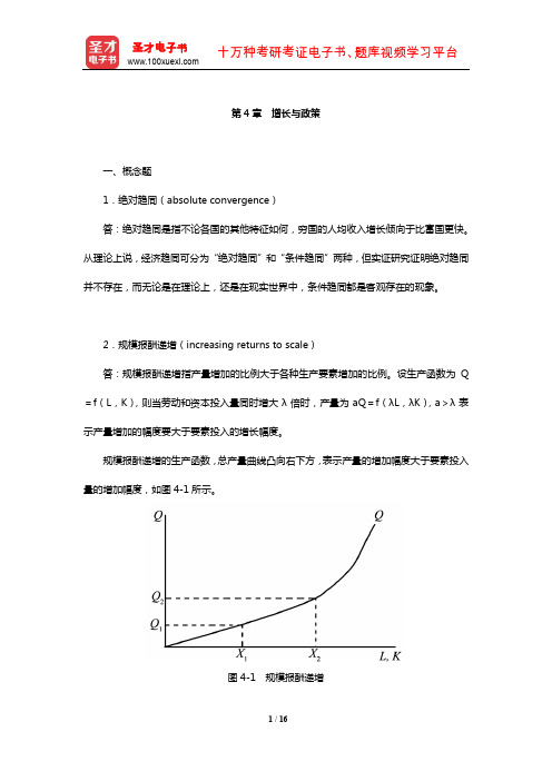
规模报酬递增的生产函数,总产量曲线凸向右下方,表示产量的增加幅度大于要素投入量的增加幅度,如图4-1所示。
图4-1 规模报酬递增图4-1中,横轴表示劳动L和资本投入量K,纵轴表示产量Q,曲线Q为总产量曲线。
当各种要素投入量由X1增加到X2时,引起产量由Q1增加到Q2,要素投入量增加了一倍,而产量的增加大于一倍。
产生规模报酬递增的主要原因是企业生产规模扩大所带来的生产效率的提高。
它可以表现为:生产规模扩大以后,企业能够利用更先进的技术和机器设备等生产要素,而较小规模的企业可能无法利用这样的技术和生产要素。
随着对较多的人力和机器的使用,企业内部的生产分工能够更加合理和专业化。
此外,人数较多的技术培训和具有一定规模的生产经营管理也可以节省成本。
3.稳定均衡(stable equilibrium)答:稳定均衡指如果经济体系的均衡状态遭到暂时破坏时,依靠其自身的力量最终还会恢复到原来所处的均衡状态的一种均衡。
其特点是一个经济体系的均衡状态,在制约它的各种外部条件发生变动时,会使该经济体系产生脱离均衡状态的运动,但是,经济体系内部又同时会自动地产生一种力量,这种力量使体系中的各种变量重新恢复到原来的均衡状态。
例如,当某一商品的供给曲线在均衡点的斜率大于需求曲线的斜率时,脱离均衡状态的波动幅度会自动逐渐缩小以至消失,并最终停留在原均衡点上,这就是阐述动态均衡的蛛网理论所描述的收敛型蛛网情况。
宏观经济学课后习题答案
宏观经济学课后习题答案问题1:什么是宏观经济学?它的研究对象是什么?宏观经济学是一门研究整体经济运行的学科。
它关注的是经济中的总体现象和经济运行的规律,包括国民经济的总体规模、增长速度、物价水平、就业水平、物资供求关系等。
宏观经济学的研究对象是整个经济系统,即国民经济的各个部门和各个经济主体之间的关系。
问题2:GDP的定义是什么?它的计算方法有哪些?GDP(国内生产总值)是一个国家或地区在一定时间内所生产的最终产品和服务的总价值。
它可以通过产出法、收入法和支出法进行计算。
•产出法:根据产品的产出量和售价来计算GDP。
主要包括产业增加值、商品增值税和净关税三个部分。
产业增加值是国内企业生产商品和服务所增加的价值,商品增值税是销售商品过程中增加的税费,净关税是进口商品关税减去出口商品的关税。
•收入法:根据国民收入的构成来计算GDP。
主要包括工资、利润、利息和租金等因素。
•支出法:通过对整体需求的衡量来计算GDP。
主要包括消费支出、投资支出、政府支出和净出口四个部分。
问题3:什么是通货膨胀?它有哪些影响因素?通货膨胀是指货币购买力下降,物价水平普遍上涨的现象。
通货膨胀导致货币价值的贬值,影响经济体制和社会生活的稳定。
通货膨胀的影响因素包括:1.需求拉动型通货膨胀:需求过高导致价格上涨。
当居民收入增加,需求上升,商品供不应求时,市场价格会上涨,从而导致通货膨胀。
2.成本推动型通货膨胀:成本上升导致价格上涨。
生产成本的上升,如劳动力成本、原材料成本等,将推动产品价格上涨,从而导致通货膨胀。
3.货币发行过多:当国家通过货币发行扩大经济增长,而没有相应的经济增长,会导致货币供应过剩,从而出现通货膨胀。
4.供给不足:当出现自然灾害、生产能力下降或政策限制等因素,会导致供给不足,进而推动商品价格上涨,引发通货膨胀。
问题4:什么是经济增长?有哪些推动经济增长的因素?经济增长指的是一个国家或地区在一定时间内经济总量的扩大。
16宏观经济学英文版(多恩布什)课后习题答案全解

CHAPTER 16THE FED, MONEY, AND CREDITSolutions to the Problems in the Textbook:Conceptual Problems:1. The three tools the Fed has to conduct monetary policy are open market operations, discount ratechanges, and reserve requirement changes. If the Fed wants to increase the money supply, it has the following options: first, the Fed can buy government bonds from the public (mostly banks), thereby increasing bank reserves. These open market purchases will induce banks to extend their loans, which will create more money. Second, it can lower the discount rate, so it becomes less costly for banks to borrow reserves from the Fed. This also will induce banks to create more money by extending more loans. Finally, the Fed can lower the required-reserve ratio, which again will allow banks to lend more.2. The currency-deposit ratio is the ratio of currency outstanding to bank deposits. The Fed cannotdirectly influence this ratio, since it is determined by the behavior of the public and influenced by the convenience of obtaining cash and by seasonal patterns (increased Christmas shopping, for example).However, by changing either bank regulations (that would affect the ease of obtaining cash) or interest rates (that would change the opportunity cost of holding cash), the Fed may indirectly affect how much currency the public is willing to hold.3.a. 3.a.ii2i2i1 i10 0Y2 Y1 Y Y1 Y2 YIf most disturbances come from the money sector (a shift in money demand), interest rate targets work better than money targets. In the IS-LM diagram below we can see that as money demand increases due to changing expectations, the LM-curve will shift to the left and the interest rate will increase. By increasing money supply and shifting the LM-curve back to the right, the central bank can get the economy back to the original equilibrium.3.b. If most disturbances come from the expenditure sector, the central bank is better off targeting moneysupply. If spending increases, the IS-curve shifts to the right and the interest rate increases. If the central bank tried to get the interest rate back to its original level by increasing money supply, the disturbance would intensify, since the LM-curve would also shift to the right. Thus, the central bank should keep money supply (and thus the LM-curve) stable to keep the disturbance at a minimum.4.a. A bank run occurs when depositors, worried about the safety of their assets, rush to withdraw theirdeposits.4.b. If a bank is in trouble because it has made some bad investment decisions, people may expect it tofail. Thus they may want to withdraw their deposits before it is too late. Since other depositors are1likely to behave in the same way, a run on the bank can be anticipated. Even a fairly financially sound bank may not be able to withstand a run, since most assets are tied up in loans. Almost all U.S. banks are FDIC insured and therefore a run on a bank is very unlikely. With FDIC insurance, depositors know that they can get at least their principal back from the government should a bank fail, and therefore they do not panic easily.4.c. During the Great Depression, a large-scale run on banks lead to liquidity problems and bank failures.This decreased the lending power of the whole banking system. In other words, depositors lost their confidence in banks and withdraw their deposits. This increased the currency-deposit ratio, leading toa decrease in the money multiplier and a contraction in money supply.4.d. The existence of the FDIC increases the public's confidence in the banking system, so a run on banksis highly unlikely. Therefore the currency-deposit ratio is low and the value of the money multiplier is high. The money multiplier is also more stable since the public does not withdraw deposits any time a bank failure occurs.5.a. There are basically two reasons why the Fed does not adhere more closely to its monetary growthtargets in the short run. The first is technical: due to the variability of the money multiplier and the lag in collecting data on money supply figures, the Fed is not always able to achieve its monetary growth target. The second reason is that the Fed, in the short run, uses interest rate targets concurrently with monetary growth targets, and it is impossible to succeed at both at the same time. Therefore, as the Fed responds to changes in the economy, it may move away at least temporarily from its monetary growth target. The Fed's desire to have some short-run flexibility while still maintaining long-run credibility, may cause a temporary deviation from the announced monetary growth target.5.b. The targeting of nominal interest rates can be self-defeating, especially in times of high inflation. If(nominal) interest rates increase, the Fed has to increase money supply to reduce interest rates to their original level. However, expansionary monetary policy will lead to more inflation and this will ultimately result in higher nominal interest rates. The so-called Fisher-equation states that the nominal interest rate (i n) is equal to the real interest rate (i r) plus the rate of inflation (π), that is,i n = i r + π.In the long run, the real interest rate will not be affected by expansionary monetary policy, but the nominal interest rate will be higher due to increased inflation. Another attempt to further reduce the nominal interest rate by expanding money supply even more will aggravate inflation even more and ultimately not succeed in bringing interest rates down.6.a. Nominal GDP is an ultimate target of monetary policy.6.b. The discount rate is an instrument of monetary policy.6.c. The monetary base is an immediate target of monetary policy.6.d. M1 is an intermediate target of monetary policy.6.e. The Treasury bill rate is an intermediate target of monetary policy.6.f. The unemployment rate is an ultimate target of monetary policy.7. When banks ration credit, interest rates are no longer a good indication of existing market conditions.Credit is rationed when lending institutions limit the amount that their customers can borrow based on concerns that such borrowing may not be financially prudent. In this situation, the Fed should not use interest rate targets as a guide for its monetary policy, since interest rates no longer reflect true market conditions.8. The Fed has much more control over intermediate targets (money supply or interest rates) than it doesover ultimate targets (GDP, unemployment, or inflation). Changes in these intermediate targets do not have an immediate effect on the ultimate targets and therefore the Fed can easily reverse or re-enforce its policy measure. Because of the long lags associated with monetary policy, the Fed uses these2intermediate targets to get feedback on the effects of a policy change and the likeliness that a policy measure will achieve its ultimate goal. However, concentrating solely on intermediate targets does not guarantee that the ultimate objectives will be achieved.9. From the quantity theory of money equation MV = PY, we get%∆M + %∆V = %∆P + %∆Y ==> %∆P = %∆M - %∆Y + %∆V.If real GDP (Y) is assumed to grow at a rate of 3.5%, the Fed has to let money supply (M) grow at a rate of 3.5% to keep prices (P) stable, assuming that velocity (V) remains stable. The Fed can control nominal GDP through changes in nominal money supply only as long as the behavior of money demand (and thus velocity) is relatively predictable. The long-run GDP growth rate has been around2.25%, far below the3.5% mentioned here, and expansionary monetary policy will not achieve such ahigh growth rate. But there is a very close relationship between money supply changes and price changes in the long run, while real GDP growth is primarily influenced by other factors. If the Fed overestimates the rate at which potential GDP grows, then it is likely to stimulate the economy too much and induce high inflation. Therefore, nominal GDP targeting rather than real GDP targeting may be a better approach, since the former creates a policy tradeoff between unemployment and inflation. In other words, we will get less growth but also less inflation if potential GDP growth is overestimated.Technical Problems:1. Assume the Fed sells Treasury bills valued at $10 million to a bank.Fed Balance Sheet: Assets LiabilitiesGovt. securities - $10 Currency 0Other assets 0 Bank deposits - $10 Bank Balance Sheet: Assets LiabilitiesDeposits at the Fed - $10 Deposits 0Govt. securities + $10Other assets 0The bank has now lost $10 million in reserves (deposits at the Fed). If required reserves are no longer sufficient, then the bank will have to acquire new reserves.If a bank depositor buys the Treasury bills, then the balance sheet will be:Bank Balance Sheet: Assets LiabilitiesReserves - $10 Deposits - $10Other assets 0Again, the bank may have to make up for the loss of reserves.2. Assume the Fed buys $10 million worth of gold and then decides to sterilize the effect of thispurchase on the monetary base through open market operations.Fed Balance Sheet: Assets LiabilitiesGold + $10 Currency 0Other assets 0 Member bank deposit + $10 The purchase of gold increased the monetary base (bank reserves) by $10 million.Fed Balance SheetAfter Sterilization: Assets LiabilitiesGold + $10 Bank deposits (+10 -10) = $0Govt. securities - $103The sale of government securities to banks again decreased the monetary base (bank reserves) by $10 million, so there is no overall change in the monetary base.3.a. If the reserve-deposit ratio is 100%, then banks cannot create any loans and the money multiplier isequal to 1. This means that the Fed has total control over the money supply, since it has control over bank reserves. However, this would significantly change the banking industry, since banks no longer would be able to extend loans.3.b. Since banks would not be able to issue any loans, the assets side would contain only reserves.3.c. Banking could still remain profitable as long as banks were able to generate service charges to covertheir operating costs.4.In deciding whether monetary base targeting or interest rate targeting is better for the Fed in itsconduct of monetary policy, it would be good to know whether the goods sector or the money sector is more prone to disturbances. If most disturbances occur in the goods sector (assume the IS-curve shifts to the right), then monetary base targeting is better, since interest rate targets would force the Fed to aggravate the disturbance. Under interest rate targeting, the Fed would be forced to change money supply (shifting the LM-curve to the right) and aggregate demand would be changed even more. If most disturbances occur in the money sector (assume the LM-curve shifts to the left), then interest rate targeting is better, since the Fed can easily offset the disturbance. Under interest rate targeting the Fed could change money supply (shifting the LM-curve to the right again) without affecting aggregate demand.ii2i2i1 i1Y2 Y1 Y Y1 Y2 YAdditional Problems:1. How does an increase in the currency-deposit ratio affect the money multiplier? What is theeffect of an increase in the reserve-deposit ratio?The money multiplier is defined as mm = (1 + cu)/(cu + re), wherecu = CU/D = currency-deposit ratio, andre = R/D = reserve-deposit ratio.An increase in the currency-deposit ratio means that people hold more currency and banks have fewer funds to create deposits. Therefore the money multiplier decreases. An increase in the reserve-deposit ratio means that banks now hold more reserves, so fewer deposits can be created. Again, the money multiplier decreases.42. Assume that an increasing number of department and grocery stores accept credit and debitcards and more consumers use these cards to do their shopping. How will the money multiplier and money supply be affected?If more consumers make purchases using credit or debit cards rather than cash, then less currency is held and the currency-deposit ratio will be lower. This implies a larger money multiplier and, given a fixed stock of high-powered money, an increase in money supply.3. "The introduction of the FDIC after the Great Depression not only calmed the worries of thepublic but also made monetary policy easier for the Fed." Comment on this statement.The introduction of the FDIC lowered the public's fear of new bank failures. Consumer confidence in the banking system increased and people held less currency. Banks also were able to reduce their excess reserves, since they no longer feared a widespread bank run. The currency-deposit and the reserve-deposit ratios both declined, and the size of the money multiplier increased. In addition, the money multiplier became more stable, since consumers became less likely to panic after a bank failure occurred. The larger and the more stable the money multiplier, the easier it is for the Fed to control money supply by changing the monetary base through open market operations.4. Assume money supply (M) is $1,200 billion, total bank deposits (D) are $800 billion and therequired reserve-deposit ratio is 10%. What would the Fed have to do to lower money supply by 5%? Explain your answer.We know that M = CU + D ==> CU = M - D = 1,200 - 800 = 400.If we assume that banks do not hold excess reserves, thenR = (0.1)D = (0.1)800 = 80 and H = CU + R = 400 + 80 = 480.Thus the money multiplier is M/H = mm = 1,200/480 = 2.5.If the Fed wants to reduce money supply by 5% or $60 billion, it has to reduce high-powered money (H) by $24 billion, by selling $24 billion worth of Treasury bills. In other words,∆M = mm(∆H) == > - 60 = 2.5(∆H) ==> (∆H) = - 60/2.5 = - 245. Assume the currency-deposit ratio is 30%, the required reserve-deposit ratio is 8% and theexcess reserve-deposit ratio is 2%. How much would money supply change if the Fed made open market sales valued at $20 million?The money multiplier is defined as: M/H = mm = (1 + cu)/(cu + re).In this example the size of the money multiplier is equal tomm = (1 + 0.3)/(0.3 + 0.08 + 0.02) = (1.3)/(0.4) = 3.25.An open market sale valued at $20 million would decrease high-powered money (H) by $20 million. Therefore, money supply (M) would decrease by $65 million, since∆M = mm(∆H) = (3.25)(-20) = - 65.6. Assume bank deposits are $3,200 billion, the required reserve-deposit ratio is 10%, andcurrency outstanding is $400 billion. What should the Fed do to decrease money supply by $100 million?Ms = Cu + D = 400 + 3,200 = 3,600 and H = Cu + R = Cu + (0.1)D = 400 + 320 = 720==> money multiplier = Ms/H = mm = 3,600/720 = 5==> ∆Ms = mm(∆H) ==> - 100 = 5(∆H) ==> ∆H = - 20If the Fed wants to decrease money supply by $100 million, bank reserves have to be decreased by $20 million through the open market sale of government securities. (Note: The assumption was that excess reserves are zero, which may not be true.)7. True or false? Why?5"An open market sale raises the monetary base and therefore money supply."False. An open market sale occurs when the Fed sells government bonds to the private sector, primarily banks, in return for currency. Reserves held in the form of deposits at the Fed decrease, and therefore the monetary base (the stock of high-powered money) decreases as does money supply, since banks cannot loan out as much as previously.8. What problems would arise if the Fed tried to conduct open market operations via the stockmarket?Theoretically, the Fed could change high-powered money and thus the supply of money by buying and selling stocks. The problem, however, would be how to decide which stocks to buy and sell, since the Fed's actions would affect the values of the stocks being bought or sold.9. "Large open market sales may have a negative impact on the demand for money, the budgetsurplus, the income velocity of money, and consumption." Comment on this statement.Open market sales decrease bank reserves and therefore money supply. This increases interest rates, leading to a lower level of investment and income. Since income tax revenues decrease in a recession, the budget surplus will also decrease. Since interest rates are higher, the interest payments on the national debt will increase. A lower level of income means a lower level of consumption. The income velocity of money generally declines in a recession. However, the decline in money occurs before the decline in income. Thus we first see an increase in velocity in the short run, followed by a decrease.10. Which is the most useful tool for the Fed to conduct its monetary policy? In your answerdiscuss the advantages and disadvantages of each of the tools that the Fed has at its disposal. The Fed has three basic tools to conduct monetary policy are open market operations, discount rate changes, and reserve requirement changes.Open market operations are used most often by the Fed since it can be undertaken every business day, can be undertaken to a large or small degree, and can be easily reversed. Bank reserves are immediately affected to a desired degree with the initiative lying solely with the Fed.The discount rate can be used as a signal for a change in monetary policy, but often a change in the discount rate simply reflects an adjustment to existing money market conditions. The disadvantage of using the discount rate is that it is up to banks to change the level of bank reserves. Bank reserves only change when banks borrow more or less from the Fed. Since this behavior cannot be anticipated, bank reserve changes cannot be accurately anticipated.Reserve requirement changes are used only rarely, since this is an extremely blunt tool. A reserve requirement change will affect the money multiplier and have a huge effect on money supply. Generally banks are given ample time to adjust to changes.11. Comment on the following statement:"Changes in the discount rate are always a sign that the Fed has changed its monetary policy." The discount rate is the rate at which banks can borrow from the Fed. The federal funds rate is the rate at which banks can borrow from each other. Banks generally prefer to borrow at the lowest rate. They do not like to borrow too often or too much from the Fed, however, since the Fed may then question their way of doing business. But if the demand for bank reserves increases and the difference between the federal funds rate and the discount rate gets too large, banks have an incentive to borrow from the Fed more often than usual. In this case total bank reserves will increase more than the Fed would like. As a result, the Fed may adjust the discount rate to bring it more in line with the federal funds rate. Therefore, while an increase in the discount rate may signal a shift in the Fed's policy, it may also simply reflect the Fed's response to a change in money market conditions.612. In 1991-92, the Fed repeatedly lowered the discount rate, but failed to stimulate the economy.Explain this fact. Subsequently, the Fed lowered the reserve requirements for banks. In your opinion, what was the Fed's objective in doing this, and was the objective achieved?Lowering the discount rate is not always successful in increasing money supply (and thus stimulating the economy), since it requires that banks take the initiative to change bank reserves. In 1991-92, the U.S. was in a recession and negative business expectations persisted. Many banks needed to recover from loan losses they had incurred and did not want to extend credit even though they were encouraged to do so by the Fed.The Fed finally lowered the reserve requirements for banks in a further effort to stimulate the economy but also to increase the profitability of banks. Banks do not earn interest on the reserves they hold, so a decrease in reserve requirements allowed them to increase their earnings and reduce their portfolio risk by buying Treasury-bills. While the economy was not immediately stimulated by new loans, at least the profitability of banks increased, creating more stability within the banking system.13. "Open market sales are more effective than increasing the discount rate in changing moneysupply." Comment. In your answer explain the short-run effects of restrictive monetary policy on velocity, the budget surplus, and national saving.With open market operations, the Fed has the initiative and bank reserves are immediately affected. Open market operations can be undertaken to a small or large extent on every business day, the Fed can determine the level of impact on bank reserves, and the Fed's actions can be easily reversed. Discount rate changes affect banks' cost of borrowing from the Fed, but leave the initiative to react to the banks. Thus, the Fed cannot easily predict the exact effect on bank reserves. For example, in 1991 the Fed changed the discount rate 15 times but banks did not borrow more from the Fed or increase their lending due to unfavorable economic conditions. If the Fed restricts money supply, interest rates will increase, leading to a decrease in economic activity. Initially, the income velocity (V = PY/M) will increase due to the lower money supply (M), but it will take time to affect income. But as national income (Y) decreases, income velocity will decline. Other results will include a decrease in the budget surplus (due to lower tax revenues) and national saving (due to lower income and a lower government surplus).14. Assume the Fed lowered the discount rate. How would personal saving, the budget surplus andaggregate money demand be affected?A lower discount rate is intended to encourage banks to borrow more from the Fed. It is not always clear that banks will respond as expected, but if they do, bank reserves will increase and so will money supply, as banks increase their lending activity. This will lower interest rates, leading to an increase in investment and national income. Personal saving will increase with a higher income level. Similarly, tax revenues will go up, increasing the budget surplus. Lower interest rates and higher income will increase money demand. (We also can see this from the fact that money supply has increased. Since the money sector has to move into a new equilibrium, money demand has to go up if money supply is increased.)15. Should you expect the federal funds rate to be above the discount rate or vice versa? Explain. The Fed is the lender of last resort and banks can always borrow from the Fed if the need arises. When banks borrow from the Fed, they are charged a rate called the discount rate. But banks also have the option to borrow from each other at the federal funds rate. Banks generally prefer to borrow at the lowest rate possible. However, they do not like to borrow too heavily from the Fed, since the Fed is a regulator of banks. Banks fear that their behavior will be questioned if the Fed takes notice and thus prefer to borrow from each other. In doing so, they drive the federal funds rate above the discount rate.716. "Reserve requirements act as an unfair tax on banks." Comment on this statement.Banks are forced to hold their reserves either as vault cash or as deposits at the Fed earning no interest in either case. Since other financial institutions have no such reserve requirement, it could be argued that this unfairly taxes banks. On the other hand, reserves guarantee a certain amount of liquidity for the banking system, which may be necessary, should there be a run on banks. The reserves held as deposits at the Fed also serve to facilitate the check clearing process. For these reasons, the tax can be viewed as necessary and therefore less "unfair."17. Does the Fed have control over the federal funds rate and over bank reserves? If so, can the Fedcontrol both simultaneously?The Fed has indirect control over the federal funds rate, since it has control over the supply of total bank reserves in the banking system through open market operations. However, the Fed cannot control the demand for bank reserves. If the demand for bank reserves increases, the federal funds rate will rise. If the Fed chooses to peg the federal funds rate, it has to create additional bank reserves via open market purchases. On the other hand, if the Fed chooses to control the level of bank reserves, it has to let the federal funds rate fluctuate. Therefore, the Fed cannot control the federal funds rate and the level of bank reserves simultaneously.18. "By lowering the reserve requirements for banks, the Fed reduces the budget deficit, nationalsaving, and the income velocity of money." Comment on this statement.If the Fed lowers the reserve requirement, banks have more money to lend out and can thus increase their earnings by making more loans or buying T-bills. If banks extend their loans, then money supply will increase and interest rates will decrease, stimulating investment and national income. Saving will increase with a higher level of income. Similarly, tax revenues will go up, reducing the budget deficit. Interest payments on the national debt will also decrease with lower interest rates, which will also help to lower the deficit. Velocity will initially decrease, since money supply will increase before income. But as income increases, then velocity will increase again. Ultimately, velocity may not change by much, since the income elasticity of money demand is close to one in the long run.19. "Restrictive monetary policy over a long time period will lead to lower interest rates."Comment on this statement.Long-run effects of monetary policy are different from short-run effects. Restrictive monetary policy leads to higher interest rates in the short run due to less liquidity (liquidity effect). But higher interest rates will reduce aggregated demand, which reduces prices and national income. Thus the level of interest rates will start to decline again (price-income effect). Lower prices will eventually lead to lower inflationary expectations and thus lower nominal interest rates (price-anticipation effect). In the end, real interest rates (i r) will return to their original level and nominal interest rates (i n) will be lower, since the inflation rate (π) is lower. This is shown in the so-called Fisher equation: i n = i r + π.20. "The elimination of required reserves on bank deposits would decrease the Fed's control overmoney supply. But if money supply increased uncontrollably, then high rates of inflation would result." Comment on the following statement.The Fed has a number of policy instruments at its disposal to control the level of bank reserves (and thus money supply). The required-reserve ratio is only one such instrument. The Fed can always influence bank reserves through the use of open market operations. Even if reserve requirements are abolished, the money multiplier will always have a finite value, since banks will always hold some (excess) reserves to meet their daily cash needs and emergency needs. If the reserve requirement were eliminated, the money multiplier would become larger, since banks would not choose to voluntarily hold as many reserves as the Fed required. However, large-scale open market operations would still enable the Fed to exercise great influence over bank reserves and therefore money supply.8。
多恩布什《宏观经济学》课后习题详解(衰退与萧条)【圣才出品】
第21章衰退与萧条一、概念题1.大萧条(Great Depression)答:大萧条指1929年至1939年之间发生的全球性经济大衰退,是以商业和经济运营普遍衰退为特征的一种经济状况。
1929~1933年的萧条——“世界经济衰退”比任何一次经济衰退的影响都要深远得多。
这次经济萧条是以农产品价格下跌为起点的,农业衰退由于金融的大崩溃而进一步恶化,尤其在美国,一股投机热导致大量资金从欧洲抽回,随后在1929年10月发生了令人恐慌的华尔街股市暴跌。
在全球范围内,经济衰退造成大规模的持续失业;资本的短缺在所有的工业化国家中都带来了出口和国内消费的锐减;这场灾难还使中欧和东欧许多国家的制度遭到破产。
根据凯恩斯的理论,大萧条是因为有效需求不足而产生的,所以政府的任务是扩大有效需求。
2.大衰退(Great Recession)答:大衰退指的是一场在2007年8月9日开始浮现的金融危机引发的经济衰退,始于美国房地产市场,不断深化并传播到全球,从金融市场传递到商品和服务市场。
大量的低成本抵押贷款,特别是给那些收入太低而不足以支付所购买房屋者的贷款,导致了房价的疯狂上涨。
只要房屋价格继续上涨,房屋所有人就能通过再融资偿还最初的抵押贷款。
当然,一旦房价停止上涨,房屋所有人将只剩下他们难以偿付的贷款,而且不能再融资。
大部分银行通过抵押贷款证券化在金融市场卖掉了抵押贷款。
而当存在真实风险时这些证券被作为无风险证券交易,加上金融衍生品的繁荣发展并被那些对赌注风险毫不知情的投资者不断交易,导致了次级房屋信贷危机的爆发,投资者开始对按揭证券的价值失去信心,引发了大衰退。
3.新政(New Deal)答:新政又称“罗斯福新政”,指面对1929~1933年的世界经济大危机,1933年罗斯福接任美国总统后为挽救经济所采取的一系列社会、经济政策的总称。
新政主要包括通过国会制定了《紧急银行法令》《国家产业复兴法》《农业调整法》等法案,其主旨是强化政府干预,通过采取一系列发展国家垄断资本主义的措施来克服严重的信贷危机及经济衰退。
多恩布什宏观经济学答案

Chapter 2 national income accountingTechnical Problems1.The text calculates the change in real GDP in 1996 prices in the following way:[RGDP04 - RGDP96]/RGDP96 = [3.50 - 1.50]/1.50 = 1.33 = 133%.To calculate the change in real GDP in 2004 prices, we first have to calculate the GDP of 1996 in 2004 prices.Thus we take the quantities consumed in 1996 and multiply them by the prices of 2004, as follows:B eer 1 at $2.00 = $2.00Skittles 1 at $0.75 = $0.75_______________________________Total $2.75The change in real GDP can now be calculated as [6.25 - 2.75]/2.75 = 1.27 = 127%.We can see that the growth rate of real GDP calculated this way is roughly the same as the growth rate calculated above.2.a. The relationship between private domestic saving, private domestic investment, the budget deficit, and netexports is shown by the following identity:S - I ≡ (G + TR - TA) + NX.Therefore, if we assume that transfer payments (TR) remain constant, an increase in taxes (TA) has to be offset either by an increase in government purchases (G), an increase in net exports (NX), or a decrease in the difference between private domestic saving (S) and private domestic investment (I).2.b.From the equation YD ≡ C + S it follows that an increase in disposable income (YD) will be reflected in anincrease in consumption (C), saving (S), or both.2.c.From the equation YD ≡ C + S it follows that when either consumption (C) or saving (S) increases, disposableincome (YD) must increase as well.3.a. Since depreciation is defined as D = I g - I n = 800 - 200 = 600 ==>NDP = GDP - D = 6,000 - 600 = 5,400.3.b.From GDP = C + I g + G + NX ==> NX = GDP - C – I g - G ==>NX = 6,000 - 4,000 - 800 - 1,100 = 100.3.c.BS = TA - G - TR ==> (TA - TR) = BS + G ==> (TA - TR) = 30 + 1,100 = 1,1303.d.YD = Y - (TA - TR) = 6,000 - 1,130 = 4,8703.e. S = YD - C = 4,870 - 4,000 = 8704.a. S = YD - C = 5,100 - 3,800 = 1,3004.b.From S - I = (G + TR - TA) + NX ==> I = S - (G + TR - TA) - NX = 1,300 - 200 - (-100) = 1,200.2704.c.From Y = C + I + G + NX ==> G = Y - C - I - NX ==>G = 6,000 - 3,800 - 1,200 - (-100) = 1,100.Also: YD = Y - TA + TR ==> TA - TR = Y - YD = 6,000 - 5,100 ==> TA - TR = 900From BS = TA - TR - G ==> G = (TA - TR) - BS = 900 - (-200) ==> G = 1,100.5.According to Equation (2) in the text, the value of total output (in billions of dollars) can be calculated as: Y =labor payments + capital payments + profits = $6 + $2 + $0 = $8.6.a.Since nominal GDP is defined as the market value of all final goods and services currently produced in thiscountry, we can only measure the value of the final product (bread), and therefore we get $2 million (since 1 million loaves are sold at $2 each).6.b.An alternative way of measuring GDP is to calculate all the value added at each step of production. The totalvalue of the ingredients used by the bakeries can be calculated as:1,200,000 pounds of flour ($1 per pound) = 1,200,000100,000 pounds of yeast ($1 per pound) = 100,000100,000 pounds of sugar ($1 per pound) = 100,000100,000 pounds of salt ($1 per pound) = 100,000__________________________________________________________= 1,500,000Since $2,000,000 worth of bread is sold, the total value added at the bakeries is $500,000.7.If the CPI increases from 2.1 to 2.3, the rate of inflation can be calculated in the following way:rate of inflation = (2.3 - 2.1)/2.1 = 0.095 = 9.5%.The CPI often overstates inflation, since it is calculated by using a fixed market basket of goods and services.But the fixed weights in the CPI's market basket cannot capture the tendency of consumers to substitute away from goods whose relative prices have increased. Quality improvements in goods also often are not adequately taken into account. Therefore, the CPI will overstate the increase in consumers' expenditures.8.The real interest rate (r) is defined as the nominal interest rate (i) minus the rate of inflation (π). Therefore thenominal interest rate is the real interest rate plus the rate of inflation, ori = r + π = 3% + 4% = 7%.Chapter 3Growth theory, exogenous.1.a.According to Equation (2), the growth of output is equal to the growth in lab or times labor’s share ofincome plus the growth of capital times capital’s share of income plus the rate of technical progress, that is,∆Y/Y = (1 - θ)(∆N/N) + θ(∆K/K) + ∆A/A, where2711 - θ is the share of labor (N) and θ is the share of capital (K). Therefore, if we assume that therate of technological progress is zero (∆A/A = 0), output grows at an annual rate of 3.6 percent, since ∆Y/Y = (0.6)(2%) + (0.4)(6%) + 0% = 1.2% + 2.4% = + 3.6%,1.b.The so-called "Rule of 70" suggests that the length of time it takes for output to double can becalculated by dividing 70 by the growth rate of output. Since 70/3.6 = 19.44, it will take just under 20 years for output to double at an annual growth rate of 3.6%,1.c.Now that ∆A/A = 2%, we can calculate economic growth as∆Y/Y = (0.6)(2%) + (0.4)(6%) + 2% = 1.2% + 2.4% + 2% = + 5.6%.Thus it will take 70/5.6 = 12.5 years for output to double at this new growth rate of 5.6%.2.a.According to Equation (2), the growth of output is equal to the growth in labor times the labor shareplus the growth of capital times the capital share plus the growth rate of total factor productivity, that is,∆Y/Y = (1 - θ)(∆N/N) + θ(∆K/K) + ∆A/A, where1 - θ is the share of labor (N) and θ is the share of capital (K). In this example θ = 0.3; therefore,if output grows at 3% and labor and capital grow at 1% each, we can calculate the change in total factor productivity in the following way3% = (0.7)(1%) + (0.3)(1%) + ∆A/A ==> ∆A/A = 3% - 1% = 2%,that is, the growth rate of total factor productivity is 2%.2.b.If both labor and the capital stock are fixed, that is, ∆N/N = ∆K/K = 0, and output grows at 3%, thenall the growth has to be contributed to the growth in total factor productivity, that is, ∆A/A = 3%.3.a.If the capital stock grows by ∆K/K = 10%, the effect on output will be an additional growth rate of∆Y/Y = (0.3)(10%) = 3%.3.b.If labor grows by ∆N/N = 10%, the effect on output will be an additional growth rate of∆Y/Y = (0.7)(10%) = 7%.3.c.If output grows at ∆Y/Y = 7% due to an increase in labor by ∆N/N = 10% and this increase in labor isentirely due to population growth, then per-capita income will decrease and people’s welfare will decrease, since∆y/y = ∆Y/Y - ∆N/N = 7% - 10% = - 3%.2723.d.If the increase in labor is due to an influx of women into the labor force, the overall population doesnot increase, and income per capita will increase by y/y = 7%. Therefore people's welfare (or at least their living standard) will increase.4.Figure 3-4 shows output per head as a function of the capital-labor ratio, that is, y = f(k). Thesavings function is sy = sf(k) and it intersects the (n + d)k-line, representing the investment requirement. At this intersection, the economy is in a steady-state equilibrium. Now let us assume that the economy is in a steady-state equilibrium before the earthquake hits, that is, the capital-labor ratio is currently k*. Assume further, for simplicity, that the earthquake does not affect pe oples’ savings behavior.If the earthquake destroys one quarter of the capital stock but less than one quarter of the labor force, then the capital-labor ratio will fall from k* to k1 and per-capita output will fall from y* to y1.Now saving is greater than the investment requirement, that is, sy1 > (d + n)k1, and the capital stock and the level of output per capita will grow until the steady state at k* is reached again.However, if the earthquake destroys one quarter of the capital stock but more than one quarter of the labor force, then the capital-labor ratio will increase from k* to k2. Saving (and gross investment) now will be less than the investment requirement and thus the capital-labor ratio and the level of output per capita will fall until the steady state at k* is reached again.If exactly one quarter of both the capital stock and the labor stock are destroyed, then the steady state will be maintained, that is, the capital-labor ratio and the output per capita will not change.If the severity o f the earthquake has an effect on peoples’ savings behavior, the savings function sy = sf(k) will move either up or down, depending on whether the savings rate (s) increases (if people save more, so more can be invested in an effort to rebuild) or decreases (if people save less, since they decide that life is too short not to live it up). But in either case, a new steady-state equilibrium will be reached.k1k k2 k5.a.An increase in the population growth rate (n) affects the investment requirement. As n gets larger, the(n + d)k-line gets steeper. As the population grows, increases in saving and investment will be required to equip new workers with the same amount of capital that existing workers already have.273Since the population will now be growing faster than output, income per capita (y) will decrease anda new optimal capital-labor ratio will be determined by the intersection of the sy-curve and the new(n1 + d)k-line. Since per-capita output will fall, we will have a negative growth rate in the short run.However, the steady-state growth rate of output will increase in the long run, since it will be determined by the new and higher rate of population growth.y oy1k1k o k5.b.Starting from an initial steady-state equilibrium at a level of per-capita output y*, the increase in thepopulation growth rate (n) will cause the capital-labor ratio to decline from k* to k1. Output per capita will also decline, a process that will continue at a diminishing rate until a new steady-state level is reached at y1. The growth rate of output will gradually adjust to the new and higher level n1.yy*y1t o t1tkk*k1t o t1t6.a.Assume the production function is of the formY = F(K, N, Z) = AK a N b Z c==>274∆Y/Y = ∆A/A + a(∆K/K) + b(∆N/N) + c(∆Z/Z), with a + b + c = 1.Now assume that there is no technological progress, that is, ∆A/A = 0, and that capital and labor grow at the same rate, that is, ∆K/K = ∆N/N = n. If we also assume that all available natural resources are fixed, such that ∆Z/Z = 0, then the rate of output growth will be∆Y/Y = an + bn = (a + b)n.In other words, output will grow at a rate less than n since a + b < 1, and output per worker will fall.6.b.If there is technological progress, that is, ∆A/A > 0, then output will grow faster than before, namely∆Y/Y = ∆A/A + (a + b)n.If ∆A/A < cn, output will grow at a lower rate than n, in which case output per worker will still decrease.If ∆A/A = cn, output will grow at the same rate as n, in which case output per worker will remain the same.But if ∆A/A > cn, output will grow at a rate higher than n, in which case output per worker will increase.6.c.If the supply of natural resources is fixed, then output can only grow at a rate that is smaller than therate of population growth and we should expect limits to growth as we run out of natural resources.However, if the rate of technological progress is sufficiently large, then output can grow at a rate faster than population, even if we have a fixed supply of natural resources.7.a.If the production function is of the formY = K1/2(AN)1/2,and A is normalized to 1, we haveY = K1/2N1/2 .In this case, capital's and labor's shares of income are both 50%.7.b.This is a Cobb-Douglas production function.7.c. A steady-state equilibrium is reached when sy = (n + d)k.From Y = K1/2N1/2 ==> Y/N = K1/2N-1/2==> y = k1/2 ==> sk1/2 = (n + d)k==> k-1/2 = (n + d)/s = (0.07 + 0.03)/(.2) = 1/2 ==> k1/2 = 2 = y ==> k = 4 .7.d.At the steady-state equilibrium, output per capita remains constant, since total output grows at thesame rate as the population (7%), as long as there is no technological progress, that is, ∆A/A = 0. But275if total factor productivity grows at ∆A/A = 2%, then total output will grow faster than population, that is, at 7% + 2% = 9%, so output per capita will grow at 2%.8.a.If technological progress occurs, then the level of output per capita for any given capital-labor ratioincreases. The function y = f(k) increases to y = g(k), and thus the savings function increases from sf(k) to sg(k).8.b.Since g(k) > f(k), it follows that sg(k) > sf(k) for each level of k. Therefore, the intersection of thesg(k)-curve with the (n + d)k-line is at a higher level of k. The new steady-state equilibrium will now be at a higher level of saving and output per capita, and at a higher capital-labor ratio.8.c.After the technological progress occurs, the level of saving and investment will increase until a newand higher optimal capital-labor ratio is reached. The investment ratio will increase in the transition period, since more investment will be required to reach the higher optimal capital-labor ratio.9.The Cobb-Douglas production function is defined asY = F(N, K) = AN1-θKθ.The marginal product of labor can then be derived asMP N = (∆Y)/(∆N) = (1 - θ)AN-θKθ = (1 - θ)AN1-θKθ/N = = (1 - θ)(Y/N)== > labor's share of income = [MP N*N]/Y = [(1 - θ)(Y/N)](N/Y) = (1 - θ).Chapter 4Growth theory, endogenous1.a. A production function that displays both a diminishing and a constant marginal product of capital canbe displayed by drawing a curved line (as in an exogenous growth model), followed by an upward-sloping line (as in an endogenous growth model). Such a graph is depicted below.1.b.The first equilibrium (Point A in the graph below) is a stable low-income steady-state equilibrium.Any deviation from that point will cause the economy to eventually adjust again at the same steady-state income level (and capital-output ratio). The second equilibrium (Point B) is an unstable high-income steady-state equilibrium. Any deviation from that point will lead to either a lower income steady-state equilibrium back at Point A (if the capital-labor ratio declines) or ongoing growth (if the capital-labor ratio increases). In the latter case, not only total output but also output per capita continues to grow.1.c. A model like the one in this question can be used to explain how some countries find themselves insituations with no growth and low income while others have ongoing growth and a high level of income. In the first case, a country may have invested mostly in physical capital, leading to some short-term growth at the expense of long-term growth. In the second case, a country may have invested not only in physical capital but also in human capital (education, skills, and training), reaping significant social returns.2762.a.If population growth is endogenous, that is, if a country can influence the rate of population growththrough government policies, then the investment requirement is no longer a straight line. Instead it is curved as depicted below.2.b.The first equilibrium (Point A) is a stable steady-state equilibrium. This is a situation of low incomeand high population growth, indicating that the country is in a poverty trap. The second equilibrium (Point B) is an unstable steady-state equilibrium. This is a situation of medium income and low population growth. The third equilibrium (Point C) is a stable steady-state equilibrium. This is a situation of high income and low population growth. In none of these three cases do we have ongoing growth. For any capital stock k < k B, the economy will adjust to k A, but for any capital stock k > k b (even for k > k c), the economy will adjust to k B. During the adjustment process to any of these two steady-state equilibria, the change in output per capita only will be transitory.2.c.To escape the poverty trap (Point A), a country has several possibilities: First, it can somehow find themeans to increase the capital-labor ratio above a level consistent with Point B (perhaps by borrowing funds or seeking direct foreign investment). Second, it can increase the savings rate such that the savings function no longer intersects the investment requirement curve at either Point A or Point B.Third, it can decrease the rate of population growth through specifically designed policies, such that the investment requirement shifts down and no longer intersects with the savings function at Points A or B.3.a.If we incorporate endogenous population growth into a two-sector model in Problem 2, we get acurved investment requirement line and a production function with first a diminishing and then a constant marginal product of capital as depicted below. (Note that the savings function has the same shape as the production function.)3.b. Here we should have four intersections of the savings function sf(k) and the investment requirement[n(y)+d]k. The first equilibrium (at Point A) is a stable low-income steady-state equilibrium. Any deviation from that point will cause the economy to eventually adjust again at the same steady-state income level (and capital-output ratio). The second equilibrium (at Point B) is an unstable low-income equilibrium. Any deviation from that point will lead to either a lower income steady-state equilibrium at Point A (if the capital-labor ratio declines) or a higher income steady-state equilibrium at Point C (if the capital-labor ratio increases). Since Point C is a stable equilibrium, the economy will settle back at that point again whether the capital stock increases or declines. Point D is again an unstable equilibrium but at a high level of income. Any deviation from that point will lead to either a lower income steady-state equilibrium at Point C (if the capital-labor ratio declines) or ongoing growth (if the capital-labor ratio increases).3.c.This model is more inclusive than either of the two models discussed previously and therefore hasgreater explanatory power. While the graphical analysis is far more complicated, we can now see more clearly that a poor country cannot escape the poverty trap at Point A unless it somehow succeeds in increasing the capital-labor ratio (and thus per-capita income) beyond the level at Point B.4.a.The production function is of the formY = K1/2(AN)1/2 = K1/2(4[K/N]N)1/2= K1/2(4K)1/2 = 2K.From this we can see that a = 2 since277Y = Y/N = 2(K/N) == > y = 2k.4.b.Since a = y/k = 2, it follows that the growth rate of output and capital is∆y/y = ∆k/k = g = sa - (n + d) = (0.1)2 - (0.02 + 0.03) = 0.15 = 15%.4.c.The term "a" in the equation above stands for the marginal product of capital. By assuming that thelevel of labor-augmenting technology (A) is proportional to the capital-labor ratio (k), it is implied that the level of technology depends on the amount of capital per worker that we have, which may not be realistic.4.d.In this model, we have a constant marginal product of capital and therefore we have an endogenousgrowth model.5.a.The production function is of the formY = K1/2N1/2==> Y/N = (K/N)1/2 ==> y = k1/2.From k = sy/(n + d) = sk1/2/(n +d) ==> k1/2 = s/(n + d)==> y* = s/(n + d) = (0.1)/(0.02 + 0.03) = 2==> k* = sy*/(n + d) = (0.1)(2)/(0.02 + 0.03) = 4.5.b.Steady-state consumption equals steady-state income minus steady-state saving (or investment), thatis,c* = y – sy = f(k*) - (n + d)k* .The golden-rule capital stock corresponds to the highest permanently sustainable level of consumption. Steady-state consumption is maximized when the marginal increase in capital produces just enough extra output to cover the increased investment requirement.From c = k1/2 - (n + d)k ==> (∆c/∆k) = (1/2)k-1/2 - (n + d) = 0==> k-1/2 = 2(n + d) = 2(.02 + .03) = .1==> k1/2 = 10 ==> k = 100.Since k* = 4 < 100, we have less capital at the steady state than the golden rule suggests.5.c.From k = sy/(n + d) = sk1/2/(n + d) ==> s = k1/2(n + d) = 10(0.05) = 0.5.5.d.If we have more capital than the golden rule suggests, we are saving too much and do not have theoptimal amount of consumption.Chapter 9Income and spending2781.a. AD = C + I = 100 + (0.8)Y + 50 = 150 + (0.8)YThe equilibrium condition is Y = AD ==>Y = 150 + (0.8)Y ==> (0.2)Y = 150 ==> Y = 5*150 = 750.1.b.Since TA = TR = 0, it follows that S = YD - C = Y - C. ThereforeS = Y - [100 + (0.8)Y] = - 100 + (0.2)Y ==> S = - 100 + (0.2)750 = - 100 + 150 = 50.As we can see S = I, which means that the equilibrium condition is fulfilled.1.c.If the level of output is Y = 800, then AD = 150 + (0.8)800 = 150 + 640 = 790.Therefore the amount of involuntary inventory accumulation is UI = Y - AD = 800 - 790 =10.1.d. AD' = C + I' = 100 + (0.8)Y + 100 = 200 + (0.8)YFrom Y = AD' ==> Y = 200 + (0.8)Y ==> (0.2)Y = 200 ==> Y = 5*200 = 1,000Note: This result can also be achieved by using the multiplier formula:∆Y = (multiplier)(∆Sp) = (multiplier)(∆I) ==> ∆Y = 5*50 = 250,that is, output increases from Y o = 750 to Y1 = 1,000.1.e.From 1.a. and 1.d. we can see that the multiplier is α = 5.2.a.Since the mpc has increased from 0.8 to 0.9, the size of the multiplier is now larger. Therefore weshould expect a higher equilibrium income level than in 1.a.AD = C + I = 100 + (0.9)Y + 50 = 150 + (0.9)Y ==>Y = AD ==> Y = 150 + (0.9)Y ==> (0.1)Y = 150 ==> Y = 10*150 = 1,500.2.b.From ∆Y = (multiplier)(∆I) = 10*50 = 500 ==> Y1 = Y o + ∆Y = 1,500 + 500 = 2,000.2.c.Since the size of the multiplier has doubled from α = 5 to α1 = 10, the change in output (Y) that resultsfrom a change in investment (I) now has also doubled from 250 to 500.3.a. AD = C + I + G + NX = 50 + (0.8)YD + 70 + 200 + 0 =320 + (0.8)[Y - TA + TR]= 320 + (0.8)[Y - (0.2)Y + 100] = 400 + (0.8)(0.8)Y = 400 + (0.64)YFrom Y = AD ==> Y = 400 + (0.64)Y ==> (0.36)Y = 400279==> Y = (1/0.36)400 = (2.78)400 = 1,111.11The size of the multiplier is α = 1/0.36) = 2.78.3.b.BS = tY - TR - G = (0.2)(1,111.11) - 100 - 200 = 222.22 - 300 = - 77.783.c.AD' = 320 + (0.8)[Y - (0.25)Y + 100] = 400 + (0.8)(0.75)Y = 400 + (0.6)YFrom Y = AD' ==> Y = 400 + (0.6)Y ==> (0.4)Y = 400 ==> Y = (2.5)400 = 1,000The size of the multiplier is now reduced to α1 = (1/0.4) = 2.5.3.d.The size of the multiplier and equilibrium output will both increase with an increase in the marginalpropensity to consume. Therefore income tax revenue will also go up and the budget surplus should increase. This can be seen as follows:BS' = (0.25)(1,000) - 100 - 200 = - 50 ==> BS' - BS = - 50 - (-77.78) = + 27.783.e.If the income tax rate is t = 1, then all income is taxed. There is no induced spending and equilibriumincome always increases by exactly the change in autonomous spending. In other words, the size of the expenditure multiplier is 1.From Y = C + I + G ==> Y = C o + c(Y - TA + TR) + I o + G o = C o + c(Y - 1Y + TR o) + I o + G o ==> Y = C o + cTR o + I o + G o = A o==> ∆Y = ∆A o4.On first sight, one may want to conclude that this is an application of the balanced budget theorem,since, as long as Y = 1,000, a change in the tax rate by 5% will cause total tax revenues to change by ∆TA = 50, which is the same as the change in government purchases, that is, ∆G = 50. As long as income (Y) stays the same, the budget surplus will not be affected. However, this combined fiscal policy change will have an effect on national income and, since national income goes up, so does the government’s tax revenue, due to the fact that we have income taxation. Therefore we should expect an increase in the budget surplus. This can easily be shown with a numerical example.For example, in Problem 3.d. we had a situation where the following was given:Y o = 1,000, t o = 0.25, G o = 200 and BS o = - 50.Assume now that t1 = 0.3 and G1 = 250 ==>AD' = 50 + (0.8)[Y - (0.3)Y + 100] + 70 + 250 = 370 + (0.8)(0.7)Y + 80 = 450 + (0.56)Y.From Y = AD' ==> Y = 450 + (0.56)Y ==> (0.44)Y = 450==> Y = (1/0.44)450 = 1,022.73280BS1 = (0.3)(1,022.73) - 100 - 250 = 306.82 - 350 = - 43.18 == > BS1– BS o = -43.18 - (-50) = + 6.82Therefore we see that the budget surplus has increased, since the increase in income tax revenue is larger than the increase in government purchases.5.a.While an increase in government purchases by ∆G = 10 will change intended spending by ∆Sp = 10,a decrease in government transfers by ∆TR = -10 will change intended spending by a smaller amount,that is, by only ∆Sp = c(∆TR) = c(-10). The change in intended spending equals ∆Sp = (1 - c)(10) and equilibrium income should therefore increase by∆Y = (multiplier)(1 - c)10.5.b.If c = 0.8 and t = 0.25, then the size of the multiplier isα = 1/[1 - c(1 - t)] = 1/[1 - (0.8)(1 - 0.25)] = 1/[1 - (0.6)] = 1/(0.4) = 2.5.The change in equilibrium income is∆Y = α(∆A o) = α[∆G + c(∆TR)] = (2.5)[10 + (0.8)(-10)] = (2.5)2 = 55.c.The budget surplus should increase, since the level of equilibrium income has increased and thereforethe level of tax revenues has increased, while the changes in government purchases and transfer payments cancel each other out. Numerically, this can be shown as follows:∆BS = t(∆Y) - ∆TR - ∆G = (0.25)(5) - (-10) - 10 = 1.25Chapter 10Money, interest, fiscal policy1.a. Each point on the IS-curve represents an equilibrium in the expenditure sector. (Note that this is aclosed economy, that is, NX = 0).The IS-curve can be derived by setting actual income equal to intended spending, orY = C + I + G = (0.8)[1 - (0.25)]Y + 900 - 50i + 800 = 1,700 + (0.6)Y - 50i ==>(0.4)Y = 1,700 - 50i ==> Y = (2.5)(1,700 - 50i) ==> Y = 4,250 - 125i.1.b.The IS-curve shows all combinations of the interest rate and output level such that the expendituresector (the goods market) is in equilibrium, that is, actual output equals intended spending. A decrease in the interest rate stimulates investment spending, making intended spending greater than actual output. The resulting unintended inventory decrease leads firms to increase their production until actual output is again equal to intended spending. This means that the IS-curve is downward sloping.1.c.Each point on the LM-curve represents an equilibrium in the money sector. Therefore the LM-curvecan be derived by setting real money supply equal to real money demand, that is,281M/P = L ==> 500 = (0.25)Y - 62.5i ==> Y = 4(500 + 62.5i) ==> Y = 2,000 + 250i.1.d.The LM-curve shows all combinations of the interest rate and level of output such that the moneysector is in equilibrium, that is, the demand for real money balances is equal to the supply of real money balances. An increase in income will increase the demand for real money balances. Given a fixed real money supply, this will lead to an increase in interest rates, which will then reduce the quantity of real money balances demanded until the money market clears again. In other words, the LM-curve is upward sloping.1.e.The level of income (Y) and the interest rate (i) at the equilibrium are determined by the intersectionof the IS-curve with the LM-curve. At this point, the expenditure sector and the money sector are both in equilibrium simultaneously.From IS = LM ==> 4,250 - 125i = 2,000 + 250i ==> 2,250 = 375i ==> i = 6==> Y = 4,250 - 125*6 = 4,250 - 750 ==> Y = 3,500Check: Y = 2,000 + 250*6 = 2,000 + 1,500 = 3,500i125 ISLM62,000 3,500 4,250 Y2.a.As we have seen in 1.a., the value of the expenditure multiplier is α = 2.5. This multiplier is derivedin the same way as in Chapter 9. But now intended spending also depends on the interest rate, so we no longer have Y = αA o, but ratherY = α(A o - bi) = (1/[1 - c + ct])(A o - bi) ==> Y = (2.5)(1,700 - 50i) = 4,250 - 125i.2.b.In the IS-LM model, an increase in government purchases (G) will have a smaller effect on outputthan in the model of the expenditure sector used in Chapter 9, in which interest rates are assumed to be fixed. This can be answered most easily with a numerical example. Assume that government purchases increase by ∆G = 300. The IS-curve shifts parallel to the right by==> ∆IS = (2.5)(300) = 750.Therefore, the equation of the new IS-curve is: Y = 5,000 - 125i.282。
多恩布什《宏观经济学》课后习题详解(通货膨胀)【圣才出品】
第8章通货膨胀一、概念题1.可调节利率抵押贷款(adjustable rate mortgage,ARM)答:可调节利率抵押贷款是指按照当前市场利率而自动调整利率的贷款。
可调整抵押贷款是最初在加州兴起的一种房屋贷款,后来获准在全美国使用。
该贷款利率因联邦利率的变动而跟着自动改变。
利率每六个月变动一次,但在房屋贷款的生命期中利率变化的幅度不能超过10.5%。
另外,银行必须提供客户在可调整式利率贷款和固定利率贷款之间的选择权。
2.菜单成本(menu cost)答:菜单成本指零售商对价格调整时所产生的成本负担。
厂商改变价格,需要重新印刷它的产品价格表,向客户通报改变价格的信息和理由,所有这一切都会引起一笔开支和费用。
菜单成本包括印刷新清单和目录的成本、把这些新价格表和目录送给中间商和顾客的成本、为新价格做广告的成本、决定新价格的成本,甚至还包括处理顾客对价格变动怨言的成本。
虽然菜单成本的数值并不大,但如果菜单价目表变动的次数很多,那也会给厂商带来一些不利之处,如使顾客感觉不快和麻烦等。
3.指数化(indexation)答:指数化是以条文规定的形式把工资或价格和某种物价指数联系起来,当物价上升时,工资或价格也随之上升。
比如,政府规定,工人工资的增长率等于通货膨胀率加上经济增长率。
它分为全部指数化和部分指数化两种。
全部指数化是指工资按物价上升的比例增长,部分指数化是指工资上涨的比例仅为物价上升的部分。
收入指数化政策是一种事后措施,有利于降低通货膨胀在收入分配上的影响,但对消除通货膨胀本身作用并不大。
严格来说,指数化并不能构成一种反通货膨胀的方法。
4.完全/不能完全预期到的通货膨胀(perfectly/imperfectly anticipated inflation)答:完全预期到的通货膨胀是指通货膨胀被经济主体预期到了,并且针对这种预期采取各种补偿性行动所引发的物价上升运动。
一般认为,如果通货膨胀的预期现象普遍存在,那么无论是什么原因引起了通货膨胀,即使最初引起通货膨胀的原因消除了,通货膨胀也会因为经济主体预期而采取的行动得以持续,甚至加剧。
多恩布什《宏观经济学》(英文第八版)答案-第六章
Chapter 6 Solutions to the Problems in the Textbook:Conceptual Problems:1. The aggregate supply curve and the Phillips curve describe very similar relationships and bothcurves can be used to analyze the same phenomena. The AS-curve shows a relationship between the price level and the level of output. The Phillips curve shows a relationship between the rate of inflation and the unemployment rate, given certain inflationary expectations. For example, a movement along the AS-curve depicts an increase in the price level that is associated with an increase in the level of output. As output increases, the rate of unemployment decreases (see Okun’s law).Therefore, with a larger increase in the price level (a higher level of inflation) there will be a decrease in unemployment, creating a downward-sloping Phillips curve.This downward sloping Phillips curve shifts whenever inflationary expectations change. If one assumes that workers will change their wage demands whenever their inflationary expectations change, one can conclude that a shift in the Phillips curve corresponds to a shift in the upward sloping AS-curve, since higher wages mean higher cost of production.2. In the short run, when wages and prices are assumed to be fixed, there can be no inflation and thusthe Phillips curve makes no sense over this very brief time frame. But in the medium run (in this chapter also often referred to as the short run), the Phillips curve is downward sloping as inflationary expectations are assumed to be constant. In the long run, the Phillips curve is vertical at the natural rate of unemployment, which corresponds to the vertical long-run AS-curve at the full-employment level of output.3. A variety of explanations are given in this chapter for the stickiness of wages in the short orintermediate run. One is that workers have imperfect information and nobody knows the actual price level. People don’t know whether a change in their nominal wage is the result of an increase in prices or in the real wage they receive for the work they provide. Due to this uncertainty, labor markets will not clear immediately. Another argument relies on coordination problems, that is, different firms within an economy cannot coordinate price changes in response to monetary policy changes.Individual firms change their prices only reluctantly, since they are afraid of losing market share. The efficiency wage theory argues that employers pay above market-clearing wages to motivate their workers to work harder. Firms are also reluctant to change wages because of the perceived menu costs involved. There are long-term relations between firms and workers and wages are usually set in nominal terms by wage contracts, which are renegotiated only periodically. Thus real wages fluctuate over time as the price level changes. Finally, the insider-outsider model argues that firms negotiate only with their own employees but not with unemployed workers. Since a turnover in the labor force is costly to firms, they are willing to offer above market-clearing wages to the currently employed rather than hiring the unemployed who may be willing to work for lower wages.These different views are not necessarily mutually exclusive and it is up to students to decide which of the arguments presented here they find most plausible. The explanations differ mainly in their assumption of how fast markets clear and whether employment variations are voluntary.4.a. Stagflation is defined as a period of high unemployment accompanied by high inflation.4.b. Stagflation can occur in time periods when people have high inflationary expectations. If theeconomy goes into a recession, the actual rate of inflation will fall below the expected rate of inflation.However, the actual inflation rate may still be very high while the rate of unemployment is increasing.For example, the Fed may have let money supply grow much too fast in the past, so everyone expectsa high inflation rate. If a supply shock occurs, we will see an increase in the rate of unemploymentwhile inflationary expectations and actual inflation remain very high. This scenario occurred during the 1970s. Once we have reached such a situation, it becomes necessary to design policies that will reduce inflationary expectations to shift the Phillips curve back to the left.5. Assume a disturbance occurs and the AD-curve shifts to the right. Unemployment decreases andinflation increases, and we move along the downward sloping Phillips curve to the left. However, as soon as people realize that actual inflation is higher than their inflationary expectations, they adjust their inflationary expectations upward and the downward-sloping Phillips curve shifts to the right, eventually returning unemployment back to its natural rate. In other words, the economy adjusts back at the full-employment level of income.If an adverse supply shock occurs (the upward-sloping AS-curve shifts to the left), unemployment and inflation increase simultaneously. This will correspond to a shift of the downward-sloping Phillips curve to the right. However, when people realize that actual inflation is less than expected inflation, then the downward-sloping Phillips curve starts to shift back and the economy adjusts back to the natural rate of unemployment in the long run.6.The expectations-augmented Phillips curve predicts that inflation will rise above the expected levelwhen unemployment drops below its natural rate. However, if people know that this is going to happen, why don’t they immediately adjust to it? And if people immediately adjusted to it, wouldn’t this imply that anticipated monetary policy would be ineffective to cause any deviation from the full-employment level of output? In reality, however, even if people have rational expectations, they may not be able to adjust immediately. One reason is that wage contracts often set wages for an extended time period. Similarly, prices cannot always be changed right away and the costs of changing prices may outweigh the benefits. A further argument is that even rational people make forecasting mistakes and learn only slowly.In other words, the location of the expectations-augmented Phillips curve is determined by the level of expected inflation, which is set by recent historical experience. A shift in this curve caused by changing inflationary expectations occurs only gradually. The rational expectations model, on the other hand, assumes that the Phillips curve shifts almost instantaneously as new information about the near future becomes available.Technical Problems:1. A reduction in the supply of money leads to excess demand for money and increased interest rates,reducing the level of private spending (especially investment). Therefore the AD-curve shifts to the left. This causes an excess supply of goods and services at the original price level so the price level starts to decrease. Since the AS-curve is upward sloping, a new short-run macro-equilibrium is reached at a lower level of output (and thus a higher level of unemployment) and a lower price level.PP1However, the higher level of unemployment eventually puts downward pressure on wages, reducing the cost of production and shifting the upward-sloping AS-curve to the right. Alternatively, since this equilibrium output level is below the full-employment level, prices will continue to fall, and the upward-sloping AS-curve will shift to the right. As long as output is below the full-employment level Y*, the upward-sloping AS-curve will continue to shift to the right, which means that the price level will continue to decline. Eventually a new long-run equilibrium will be reached at the full-employment level of output (Y*) and a lower price level.2. According to the rational expectations theory, an announced change in monetary policy wouldimmediately change people’s perception in regard to the expected inflation rate. If people could adjust immediately to this change in inflationary expectations, then the rate of unemployment or the output level would remain the same. In other words, we would immediately move from point 1 to point 3 in the diagram used to explain the previous question and the Fed would be unable to affect the unemployment rate. In reality, however, even if people have rational expectations and can anticipate the effects of a policy change correctly, they may not be able to immediately adjust due to wage contracts, etc. Thus, there will always be some deviation from the full-employment output level Y*.3.a. A favorable supply shock, such as a decline in material prices, shifts the upward-sloping AS-curve tothe right, leading to excess supply at the existing price level. A new short-run equilibrium is reached at a higher level of output and a lower price level. But since output is now above the full-employment level Y*, there is upward pressure on wages and prices and the upward-sloping AS-curve shifts back to the right. A new long-run equilibrium is reached back at the original position (Y*), and the original price level (assuming that the change in material prices did not affect the full-employment level of output). Since nominal wages (W) will have risen but the price level (P) will not have changed, real wages (W/P) will have increased.PP1P20 13.b. Lower material prices lower the cost of production, shifting the upward-sloping AS-curve shiftsto the right, and leading to an increase in output and a lower price level. Since unemployment is now below its natural rate, there is a shortage of labor, providing upward pressure on wages. This will increase the cost of production again, eventually shifting the upward-sloping AS-curve back to the original long-run equilibrium (assuming that potential GDP has not been affected).Additional Problems:1. Explain the long-run effect of an increase in nominal money supply on the amount of realmoney balances available in the economy.In the very short run, the price level is fixed, so if nominal money supply (M) increases, a higher level of real money balances is available, causing interest rates to fall and the level of investment spending to increase. This leads to an increase in aggregate demand. The shift to the right of the AD-curve causes the price level (P) to increase, leading to a reduction in real money balances (M/P). In the medium run (an upward-sloping AS-curve), we reach a new equilibrium at a higher output level and a higher price level. Since prices have gone up proportionally less than nominal money supply, real money balances have increased. However, to reach a new long-run equilibrium, prices have to increase further, and as a result, the level of real money balances will decrease further. When the new long-run equilibrium at Y* is finally reached, the price level will have risen proportionally to nominal money supply and the level of real money balances will be back at its original level.2. Assume the economy is in a recession. Describe an adjustment process that will ensure that theeconomy eventually will return to full employment. How can the government speed up this process?If the economy is in a recession, there will be downward pressure on wages and prices, which will bring the economy back to the full-employment output level. The upward-sloping AS-curve will shift to the right due to lower production costs. However, this process may take a fairly long time. The government can shorten this adjustment process with the help of expansionary fiscal or monetary policies to stimulate aggregate demand. The resulting shift to the right of the AD-curve implies that the final long-run equilibrium will be at a higher price level. In other words, the reduction in unemployment can only be achieved at the cost of higher inflation.3. "The stickiness of wages implies that policy makers can achieve low unemployment only if theyare willing to put up with high inflation." Comment on this statement.There are several explanations of why wages and prices adjust only slowly. One is that workers have imperfect information, so they do not realize that lower prices mean higher real wages. Another is that firms are reluctant to change prices and wages since they are unsure about the behavior of their competitors and want to avoid the perceived cost of making these changes. Finally, wage contracts tend to be long-term and staggered, so it takes time to adjust wages to price changes. Some firms may pay their workers above market-clearing wages to keep them happy and productive. For these reasons, wages and prices tend to be rigid in the short run. Thus it takes time for the economy to adjust back to full-employment.If there were a stable Phillips-curve relationship, a low rate of unemployment could only be achieved by allowing inflation to increase. However, such a stable relationship does not exist. Wages tend to be rigid in the short run, so expansionary policies lower unemployment and increase inflation in the short run. In the long run, however, the economy will adjust back to the natural rate of unemployment, so expansionary policies simply lead to a higher price level.4. "If we assume that people have rational expectations, then fiscal policy is always irrelevant.But monetary policy can still be used to affect the rate of inflation and unemployment."Comment on this statement.Individuals and firms with rational expectations consistently make optimal decisions based on all information available. As long as a policy change is anticipated, people are able to assess its long-run outcome and will try to immediately adjust. Since fiscal policy doesn't affect inflation or unemployment in the long run, it is also ineffective in the short run if wages and prices are assumed to be flexible. An anticipated change in monetary growth, on the other hand, will be reflected in a change in the inflation rate. If wages are flexible, workers will adjust their wage demands immediately and no significant change in the unemployment rate will occur. However, even if people have rational expectations, wages tend to be fairly rigid in the short run due to wage contracts. Therefore, it will take time for the economy to adjust back to a long-run equilibrium. This implies that both fiscal and monetary policy can affect the rate of inflation and unemployment to some degree in the short run.5. "Inflation cannot accelerate in a recession, when the rate of unemployment is above its naturalrate." Comment on this statement.Inflation can accelerate even in a recession, that is, when the unemployment is high, if a supply shock occurs. An oil price increase will increase the cost of production, so the upward-sloping AS-curve will shift to the left. This will increase the inflation rate and the rate of unemployment simultaneously, as firms increase their product prices and cut their production. If the Fed tries to accommodate the supply shock with expansionary monetary policy in an effort to stimulate the economy, then inflation will accelerate even more, as the AD-curve shifts to the right.6. Comment on the following statement:"The coordination approach to the Phillips curve focuses on the problems that the administration has in coordinating its fiscal policies with the monetary policies of the Fed." The coordination approach has nothing to do with fiscal or monetary policy but is simply one explanation of why wages adjust slowly. This view asserts that firms generally are unable to coordinate wage and price changes in response to a monetary policy change. For example, any firm that cuts workers' wages in response to monetary contraction while other firms don't, will anger its employees who may then choose to leave. Firms are also reluctant to change their prices since they are unsure about their competitors' behavior. Thus wages and prices change only slowly in response to a change in aggregate demand. This implies an upward-sloping (short-run) AS-curve.7. Comment on the following statement:"The unemployment rate is zero at the full-employment level of output."With a higher price level real wages decline, increasing the quantity of labor demanded. Therefore the nominal wage rate is bid up until the real wage rate is restored to its unique equilibrium level. Similarly, if prices fall, real wages increase, leading to unemployment. The nominal wage rate falls to bring the real wage rate back to its equilibrium level. So the nominal wage rate changes in proportion to the price level to maintain a real wage rate that clears the labor market. At this wage rate, the full-employment level of output is produced. However, at the full-employment output level the unemployment rate is not zero. Due to frictions in the labor market, there is always a positive unemployment rate, as workers switch between jobs. This is called the natural rate of unemployment.8. Briefly state the reason for the slow adjustment of wages to changes in aggregate demand. The reasons for the slow adjustment of nominal wages can be explained in several ways. One explanation is that workers have imperfect information, that is, they do not immediately realize whether a change in their nominal wage is the result of an increase in prices or in the real wage they receive for the work they provide. Another explanation is that coordination problems exist, that is, different firms within an economy are unsure about the behavior of their competitors and thus they only reluctantly change wages or prices. The efficiency wage theory, on the other hand, argues that firms pay above market-clearing wages to motivate their workers to work harder. Firms are also reluctant to change wages due to the perceived cost of doing so. Another argument is that wage contracts tend to be long-term, so real wages tend to fluctuate over the length of the contract and output adjusts only slowly to price changes. Finally, the insider-outsider model argues that firms negotiate only with their employees but not the unemployed. Since a turnover of the labor force is costly to firms, they are willing to offer above market-clearing wages to the currently employed rather than hiring the unemployed who may be willing to work for less. These various explanations are not mutually exclusive, and they all imply that the AS-curve is positively sloped, that is, that a change in aggregate demand will affect both output and prices in the short run.9. True or false? Why?"There is no frictional unemployment at the natural rate of unemployment."False. The natural rate of unemployment is the rate at which the labor market is in equilibrium. But there is always some unemployment due to new entrants into the labor force, people between jobs, and the like.This rate of unemployment is considered normal, due to frictions in the labor market, and is often called frictional unemployment.10. "If everyone in this economy had rational expectations, then wages would be flexible andunemployment could not occur." Comment on this statement.The new Keynesian models argue that even if people have rational expectations, socially undesirable outcomes may still occur due to imperfect competition and the existence of wage contracts. Prices may not change freely, since firms in imperfectly competitive markets are reluctant to change them, due to the menu costs involved. Nominal wages are set by contracts over a period of time, so the economy may adjust only slowly to a decrease in aggregate demand. Thus a rate of unemployment higher than the natural rate can exist over an extended period of time.11. True or false? Why?"If nominal wages were more flexible, expansionary policies would be more effective in reducing the rate of unemployment."False. In Chapter 5 we learned that in the classical case (where nominal wages are completely flexible) the AS-curve is vertical, whereas in the Keynesian case (where wages do not change, even if unemployment persists) the AS-curve is horizontal. From this we can conclude that more flexible nominal wages imply a steeper upward-sloping AS-curve. Any type of expansionary demand-side policy will shift the AD-curve to the right and this will cause the level of output and prices to increase (at least in the short-run). A steeper upward-sloping AS-curve results in a larger price increase and a smaller increase in output. But a smaller increase in the level of output results in a smaller reduction in unemployment. In either case, the economy will settle back at the full-employment level of output in the long run. In the long run, the rate of unemployment always goes back to its natural level.12. Explain the short-run and long-run effects of an increase in the level of government spendingon output, unemployment, interest rates, prices, and real money balances.An increase in government spending increases aggregate demand, shifting the AD-curve to the right. Because there is excess demand, the price level increases, which reduces the level of real money balances. Therefore interest rates increase, leading to some crowding out of investment. Due to this real balance effect, the increase in output is less than the shift in the AD-curve. Assuming an upward-sloping AS-curve, a new equilibrium is reached at a higher price level, a higher level of output, a lower unemployment rate and a higher interest rate. Since output is now above the full-employment level, wages and prices will continue to rise and the upward-sloping AS-curve will start shifting to the left. This process will continue until a new long-run equilibrium is reached at the full-employment level of income Y*, that is, until unemployment is back at its natural rate. At this point the price level, nominal wages, and interest rates will be higher than previously and real money balances will be lower.13. Briefly explain why there seems to be so much interest in finding ways to shift theupward-sloping aggregate supply curve to the right.Shifting the upward-sloping AS-curve to the right seems to be the only way to offset the effects of an adverse supply shock without any negative side effects. An adverse supply shock, such as an increase in oil prices, causes a simultaneous increase in unemployment and inflation, and policy makers have only two options for demand-management policies. Expansionary fiscal or monetary policy will help to achieve full employment faster but will raise the price level, while restrictive fiscal or monetary policy will reduce inflationary pressure but increase unemployment. Therefore, any policy that would shift the upward sloping AS-curve back to the right seems preferable, since it might bring the economy back to the original equilibrium by simultaneously lowering inflation and unemployment.14. Use an AD-AS framework to show the effect of monetary restriction on the level of output,prices and the interest rate in the medium and the long run.A decrease in nominal money supply will increase interest rates, leading to a decrease in investment spending. This will shift the AD-curve to the left, creating an excess supply of goods and services. Therefore price level will decrease and real money balances will increase. A new equilibrium will be achieved at the intersection of the new AD-curve and the upward-sloping AS-curve at an output level that is below the full-employment level.In the long run, higher unemployment will cause downward pressure on wages. As the cost of production decreases, the upward-sloping AS-curve will keep shifting to the right until a new long-run equilibrium is established at the full-employment level of output, that is, where the new AD-curve intersects the long-run vertical AS-curve at Y*. At this point, real output, the real interest rate, real money balances, and the real wage rate will be back at their original level. Nominal money supply, the price level and the nominal wage rate will all have decreased proportionally.A simplified adjustment can be shown as follows:1-->2: Ms down ==> i up ==> I down ==> Y down ==> the AD-curve shifts left ==>excess supply ==> P down ==> real ms up ==> i down ==> I up ==> Y up(The first line describes a policy change, that is, a shift in the AD-curve; the second line describes the price adjustment, that is, a movement along the AD-curve.)Short-run effect:Y down, i up, P down2-->3: Since Y < Y* ==> downwards pressure on nominal wages ==> cost of production down ==> the short run AS-curve shifts right ==> excess supply of goods ==> P down ==> real ms up==> i down ==> I up ==> Y up (This process continues until Y = Y*)Long-run effect:Y stays at Y*, i remains the same, P down.Note: Even though only one shift of the short-run AS-curve to the new long-run equilibrium is shown here, this shift is actually a combination of many shifts.P2P1P2P30 215. Briefly discuss the importance of Okun’s law in evaluating the cost of unemployment.Okun’s law states that a reduction in the unemployment rate of 1 percent will increase the level of output by about 2 percent. This relationship allows us to measure the cost to society (in terms of lost production) of a given rate of unemployment.16. True or false? Why?"If monetary policy accommodates an adverse supply shock, it will worsen any inflationary effects."True. An adverse supply shock shifts the upward-sloping AS-curve to the left. There is excess demand for goods and services at the original price level and prices start to rise, leading to lower real money balances, higher interest rates, and lower output. If no policy is implemented, then unemployment will force the nominal wage down to restore equilibrium at the original position. If the government views this adjustment process as too slow, it can respond by implementing expansionary policies. Accommodating the supply shock in this way shifts the AD-curve to the right and a new equilibrium can be reached at full-employment but at a higher price level. It is unlikely, though, that the economy will remain there for long since workers will realize that their purchasing power has been diminished by higher prices and will demand a wage increase. If they are successful, the cost of production will increase and the upward-sloping AS-curve will shift to the left again. In other words, we will enter a wage-price spiral.PP3P2P1217. Assume oil prices decline. What kind of monetary policy should the Fed undertake if its goal isto stabilize the level of output while keeping inflation low? Show with the help of an AD-AS diagram and briefly explain the adjustment process.1-->2: As oil prices decline, the cost of production decreases and the upward-sloping AS-curve shifts to the right, causing excess supply of goods. Thus the price level decreases, real money balances increase, and the interest rate declines.2-->3: A decrease in money supply will increase the interest rate, decrease private spending, and shift the AD-curve to the left. This means that prices will decrease even further and the level of output will decline. (We assume, for simplicity, that it goes back to the full-employment level Y*, so no long-run adjustment is needed.) Overall, the level of output has remained at its full-employment level but the level of prices and the interest rate have decreased.PP1P2218. Comment on the following statement:"A favorable oil shock causes lower inflation and lower unemployment."A decrease in material prices (or any other favorable supply shock) shifts theupward-sloping AS-curve to the right, and prices begin to decrease. The new equilibrium is at a lower price level and a higher level of output (a lower level of unemployment).Since output is now above the full-employment level, there will be upward pressure on nominal wages and prices, and the upward-sloping AS-curve will start shifting back to its original position (assuming that potential output was not affected). In the long run, unemployment will be back at its natural rate but the price level will have decreased (and thus real wages increased).19. “Falling oil prices will lead to increased employment, higher wage rates an dincreased real money balances.” Comment on this statement with the help of an AD-AS diagram and explain the short-run and long-run adjustment processes.A decline in material prices shifts the upward-sloping AS-curve to the right, leading to excess supply at the existing price level. A new equilibrium is reached at a higher level of output and a lower price level. But since output is now above the full-employment level Y*, there is upward pressure on wages and prices and the upward-sloping AS-curve starts shifting back to the right. A new long-run equilibrium is reached back at the original position (Y*), and the original price level (assuming that the change in material prices did not affect the full-employment level of output). Since nominal wages (W) will have risen but the price level (P) will not have changed, real wages (W/P) will have increased.PP1P2Y*Y2Y。
- 1、下载文档前请自行甄别文档内容的完整性,平台不提供额外的编辑、内容补充、找答案等附加服务。
- 2、"仅部分预览"的文档,不可在线预览部分如存在完整性等问题,可反馈申请退款(可完整预览的文档不适用该条件!)。
- 3、如文档侵犯您的权益,请联系客服反馈,我们会尽快为您处理(人工客服工作时间:9:00-18:30)。
CHAPTER 3Solutions to the Problems in the TextbookConceptual Problems:1. The production function provides a quantitative link between inputs and output. For example, theCobb-Douglas production function mentioned in the text is of the form:Y = F(N,K) = AN1-θKθ,where Y represents the level of output. (1 - θ) and θ are weights equal to the shares of labor (N) and capital (K) in production, while A is often used as a measure for the level of technology. It can be easily shown that labor and capital each contribute to economic growth by an amount that is equal to their individual growth rates multiplied by their respective share in income.2. The Solow model predicts convergence, that is, countries with the same production function, savingsrate, and population growth will eventually reach the same level of income per capita. In other words,a poor country may eventually catch up to a richer one by saving at the same rate and makingtechnological innovations. However, if these countries have different savings rates, they will reach different levels of income per capita, even though their long-term growth rates will be the same.3. A production function that omits the stock of natural resources cannot adequately predict the impactof a significant change in the existing stock of natural resources on the economic performance of a country. For example, the discovery of new oil reserves or an entirely new resource would have a significant effect on the level of output that could not be predicted by such a production function.4. Interpreting the Solow residual purely as technological progress would ignore, for example, theimpact that human capital has on the level of output. In other words, this residual not only captures the effect of technological progress but also the effect of changes in human capital (H) on the growth rate of output. To eliminate this problem we can explicitly include human capital in the production function, such thatY = F(K,N,H) = AN a K b H c with a + b + c = 1.Then the growth rate of output can be calculated as∆Y/Y = ∆A/A + a(∆N/N) + b(∆K/K) + c(∆H/H).5. The savings function sy = sf(k) assumes that a constant fraction of output is saved. The investmentrequirement, that is, the (n + d)k-line, represents the amount of investment needed to maintain a constant capital-labor ratio (k). A steady-state equilibrium is reached when saving is equal to the investment requirement, that is, when sy = (n + d)k. At this point the capital-labor ratio k = K/N is not changing, so capital (K), labor (N), and output (Y) all must be growing at the same rate, that is, the rate of population growth n = (∆N/N).6. In the long run, the rate of population growth n = (∆N/N) determines the growth rate of the steady-state output per capita. In the short run, however, the savings rate, technological progress, and the rate of depreciation can all affect the growth rate.7. Labor productivity is defined as Y/N, that is, the ratio of output (Y) to labor input (N). A surge inlabor productivity therefore occurs if output grows at a faster rate than labor input. In the U.S. we have experienced such a surge in labor productivity since the mid-1990s due to the enormous growth in GDP. This surge can be explained from the introduction of new technologies and more efficient use of existing technologies. Many claim that the increased investment in and use of computer8technology has stimulated economic growth. Furthermore, increased global competition has forced many firms to cut costs by reorganizing production and eliminating some jobs. Thus, with large increases in output and a slower rate of job creation we should expect labor productivity to increase.(One should also note that a higher-skilled labor force also can contribute to an increase in labor productivity, since the same number of workers can produce more output if workers are more highly skilled.)Technical Problems:1.a. According to Equation (2), the growth of output is equal to the growth in labor times the labor shareplus the growth of capital times the capital share plus the rate of technical progress, that is, ∆Y/Y = (1 - θ)(∆N/N) + θ(∆K/K) + ∆A/A, where1 - θ is the share of labor (N) and θ is the share of capital (K). Thus if we assume that the rate oftechnological progress (∆A/A) is zero, then output grows at an annual rate of 3.6 percent, since ∆Y/Y = (0.6)(2%) + (0.4)(6%) + 0% = 1.2% + 2.4% = + 3.6%,1.b. The so-called "Rule of 70" suggests that the length of time it takes for output to double can becalculated by dividing 70 by the growth rate of output. Since 70/3.6 = 19.44, it will take just under 20 years for output to double at an annual growth rate of 3.6%,1.c. Now that ∆A/A = 2%, we can calculate economic growth as∆Y/Y = (0.6)(2%) + (0.4)(6%) + 2% = 1.2% + 2.4% + 2% = + 5.6%.Thus it will take 70/5.6 = 12.5 years for output to double at this new growth rate of 5.6%.2.a. According to Equation (2), the growth of output is equal to the growth in labor times the labor shareplus the growth of capital times the capital share plus the growth rate of total factor productivity (TFP), that is,∆Y/Y = (1 - θ)(∆N/N) + θ(∆K/K) + ∆A/A, where1 - θ is the share of labor (N) and θ is the share of capital (K). In this example θ = 0.3; therefore, ifoutput grows at 3% and labor and capital grow at 1% each, then we can calculate the change in TFP in the following way3% = (0.3)(1%) + (0.7)(1%) + ∆A/A ==> ∆A/A = 3% - 1% = 2%,that is, the growth rate of total factor productivity is 2%.2.b. If both labor and the capital stock are fixed and output grows at 3%, then all this growth has to becontributed to the growth in factor productivity, that is, ∆A/A = 3%.3.a. If the capital stock grows by ∆K/K = 10%, the effect on output would be an additional growth rate of∆Y/Y = (.3)(10%) = 3%.3.b. If labor grows by ∆N/N = 10%, the effect on output would be an additional growth rate of∆Y/Y = (.7)(10%) = 7%.3.c. If output grows at ∆Y/Y = 7% due to an increase in labor by ∆N/N = 10%, and this increase in laboris entirely d ue to population growth, then per capita income would decrease and people’s welfare would decrease, since∆y/y = ∆Y/Y - ∆N/N = 7% - 10% = - 3%.3.d. If this increase in labor is due to an influx of women into the labor force, the overall population doesnot increase and income per capita would increase by ∆y/y = 7%. Therefore people's welfare would increase.94. Figure 3-4 shows output per head as a function of the capital-labor ratio, that is, y = f(k). The savingsfunction is sy = sf(k), and it intersects the straight (n + d)k-line, representing the investment requirement. At this intersection, the economy is in a steady-state equilibrium. Now let us assume that the economy is in a steady-state equilibrium before the earthquake hits, that is, the steady-state capital-labor ratio is currently k*. Assume further, for simplicity, that the earthquake does not affect people's savings behavior.If the earthquake destroys one quarter of the capital stock but less than one quarter of the labor force, then the capital-labor ratio falls from k*to k1 and per-capita output falls from y* to y1. Now saving is greater than the investment requirement, that is, sy1 > (d + n)k1, and the capital stock and the level of output per capita will grow until the steady state at k* is reached again.However, if the earthquake destroys one quarter of the capital stock but more than one quarter of the labor force, then the capital-labor ratio increases from k*to k2. Saving now will be less than the investment requirement and thus the capital-labor ratio and the level of output per capita will fall until the steady state at k* is reached again.If exactly one quarter of both the capital stock and the labor stock are destroyed, then the steady state is maintained, that is, the capital-labor ratio and the output per capita do not change.If the severity of the earthquake has an effect on peoples’ savings behavior, then the savings function sy = sf(k) will move either up or down, depending on whether the savings rate (s) increases (if people save more, so more can be invested in an effort to rebuild) or decreases (if people save less, since they decide that life is too short not to live it up).yy2y*y1k1 k* k2 k5.a. An increase in the population growth rate (n) affects the investment requirement, and the (n + d)k-line gets steeper. As the population grows, more saving must be used to equip new workers with the same amount of capital that the existing workers already have. Therefore output per capita (y) will decrease as will the new optimal capital-labor ratio, which is determined by the intersection of the sy-curve and the (n1 + d)k-line. Since per-capita output will fall, we will have a negative growth rate in the short run. However, the steady-state growth rate of output will increase in the long run, since it will be determined by the new and higher rate of population growth.10yy oy1k1 k o k5.b. Starting from an initial steady-state equilibrium at a level of per-capita output y*, the increase in thepopulation growth rate (n) will cause the capital-labor ratio to decline from k* to k1. Output per capita will also decline, a process that will continue at a diminishing rate until a new steady-state level is reached at y1. The growth rate of output will gradually adjust to the new and higher level n1.yy*y1t o t1 tkk*k1t o t1 t6.a. Assume the production function is of the formY = F(K, N, Z) = AK a N b Z c ==>∆Y/Y = ∆A/A + a(∆K/K) + b(∆N/N) + c(∆Z/Z), with a + b + c = 1.Now assume that there is no technological progress, that is, ∆A/A = 0, and that capital and labor grow at the same rate, that is, ∆K/K = ∆N/N = n. If we also assume that all natural resources available are fixed, such that ∆Z/Z = 0, then the rate of output growth will be11∆Y/Y = an + bn = (a + b)n.In other words, output will grow at a rate less than n since a + b < 1. Therefore output per worker will fall.6.b. If there is technological progress, that is, ∆A/A > 0, then output will grow faster than before, namely∆Y/Y = ∆A/A + (a + b)n.If ∆A/A > c, then output will grow at a rate larger than n, in which case output per worker will increase.6.c. If the supply of natural resources is fixed, then output can only grow at a rate that is smaller than therate of population growth and we should expect limits to growth as we run out of natural resources.However, if the rate of technological progress is sufficiently large, then output can grow at a rate faster than population, even if we have a fixed supply of natural resources.7.a. If the production function is of the formY = K1/2(AN)1/2,and A is normalized to 1, then we haveY = K1/2N1/2.In this case capital's and labor's shares of income are both 50%.7.b. This is a Cobb-Douglas production function.7.c. A steady-state equilibrium is reached when sy = (n + d)k.From Y = K1/2N1/2 ==> Y/N = K1/2N-1/2 ==> y = k1/2==>sk1/2= (n + d)k ==> k-1/2 = (n + d)/s = (0.07 + 0.03)/(.2) = 1/2 ==> k1/2= 2 = y ==> k = 4 .8.a. If technological progress occurs, then the level of output per capita for any given capital-labor ratioincreases. The function y = f(k) increases to y = g(k), and thus the savings function increases from sf(k) to sg(k).yy2y1128.b. Since g(k) > f(k), it follows that sg(k) > sf(k) for each level of k. Therefore the intersection of thesg(k)-curve with the (n + d)k-line is at a higher level of k. The new steady-state equilibrium will now be at a higher level of saving and output per capita, and at a higher capital-labor ratio.8.c. After the technological progress occurs, the level of saving and investment will increase until a newand higher optimal capital-labor ratio is reached. The ratio of investment to capital will also increase in the transition period, since more has to be invested to reach the higher optimal capital-labor ratio.12kk2k1t1 t2t9. The Cobb-Douglas production function is defined asY = F(N,K) = AN1-θKθ.The marginal product of labor can then be derived asMPN = (∆Y)/(∆N) = (1 - θ)AN-θKθ = (1 - θ)AN1-θKθ/N = = (1 - θ)(Y/N)==> labor's share of income = [MPN*(N)]/Y = (1 - θ)(Y/N)*[(N)/(Y)] = (1 - θ)13。