吴文贤美赛一等奖论文(2010年A题)
美国大学生数学建模竞赛优秀论文
For office use onlyT1________________ T2________________ T3________________ T4________________Team Control Number7018Problem ChosencFor office use onlyF1________________F2________________F3________________F4________________ SummaryThe article is aimed to research the potential impact of the marine garbage debris on marine ecosystem and human beings,and how we can deal with the substantial problems caused by the aggregation of marine wastes.In task one,we give a definition of the potential long-term and short-term impact of marine plastic garbage. Regard the toxin concentration effect caused by marine garbage as long-term impact and to track and monitor it. We etablish the composite indicator model on density of plastic toxin,and the content of toxin absorbed by plastic fragment in the ocean to express the impact of marine garbage on ecosystem. Take Japan sea as example to examine our model.In ask two, we designe an algorithm, using the density value of marine plastic of each year in discrete measure point given by reference,and we plot plastic density of the whole area in varies locations. Based on the changes in marine plastic density in different years, we determine generally that the center of the plastic vortex is East—West140°W—150°W, South—North30°N—40°N. According to our algorithm, we can monitor a sea area reasonably only by regular observation of part of the specified measuring pointIn task three,we classify the plastic into three types,which is surface layer plastic,deep layer plastic and interlayer between the two. Then we analysis the the degradation mechanism of plastic in each layer. Finally,we get the reason why those plastic fragments come to a similar size.In task four, we classify the source of the marine plastic into three types,the land accounting for 80%,fishing gears accounting for 10%,boating accounting for 10%,and estimate the optimization model according to the duel-target principle of emissions reduction and management. Finally, we arrive at a more reasonable optimization strategy.In task five,we first analyze the mechanism of the formation of the Pacific ocean trash vortex, and thus conclude that the marine garbage swirl will also emerge in south Pacific,south Atlantic and the India ocean. According to the Concentration of diffusion theory, we establish the differential prediction model of the future marine garbage density,and predict the density of the garbage in south Atlantic ocean. Then we get the stable density in eight measuring point .In task six, we get the results by the data of the annual national consumption ofpolypropylene plastic packaging and the data fitting method, and predict the environmental benefit generated by the prohibition of polypropylene take-away food packaging in the next decade. By means of this model and our prediction,each nation will reduce releasing 1.31 million tons of plastic garbage in next decade.Finally, we submit a report to expediction leader,summarize our work and make some feasible suggestions to the policy- makers.Task 1:Definition:●Potential short-term effects of the plastic: the hazardeffects will be shown in the short term.●Potential long-term effects of the plastic: thepotential effects, of which hazards are great, willappear after a long time.The short- and long-term effects of the plastic on the ocean environment:In our definition, the short-term and long-term effects of the plastic on the ocean environment are as follows.Short-term effects:1)The plastic is eaten by marine animals or birds.2) Animals are wrapped by plastics, such as fishing nets, which hurt or even kill them.3)Deaden the way of the passing vessels.Long-term effects:1)Enrichment of toxins through the food chain: the waste plastic in the ocean has no natural degradation in theshort-term, which will first be broken down into tinyfragments through the role of light, waves,micro-organisms, while the molecular structure has notchanged. These "plastic sands", easy to be eaten byplankton, fish and other, are Seemingly very similar tomarine life’s food,causing the enrichment and delivery of toxins.2)Accelerate the greenhouse effect: after a long-term accumulation and pollution of plastics, the waterbecame turbid, which will seriously affect the marineplants (such as phytoplankton and algae) inphotosynthesis. A large number of plankton’s deathswould also lower the ability of the ocean to absorbcarbon dioxide, intensifying the greenhouse effect tosome extent.To monitor the impact of plastic rubbish on the marine ecosystem:According to the relevant literature, we know that plastic resin pellets accumulate toxic chemicals , such as PCBs、DDE , and nonylphenols , and may serve as a transport medium and soure of toxins to marine organisms that ingest them[]2. As it is difficult for the plastic garbage in the ocean to complete degradation in the short term, the plastic resin pellets in the water will increase over time and thus absorb more toxins, resulting in the enrichment of toxins and causing serious impact on the marine ecosystem.Therefore, we track the monitoring of the concentration of PCBs, DDE, and nonylphenols containing in the plastic resin pellets in the sea water, as an indicator to compare the extent of pollution in different regions of the sea, thus reflecting the impact of plastic rubbish on ecosystem.To establish pollution index evaluation model: For purposes of comparison, we unify the concentration indexes of PCBs, DDE, and nonylphenols in a comprehensive index.Preparations:1)Data Standardization2)Determination of the index weightBecause Japan has done researches on the contents of PCBs,DDE, and nonylphenols in the plastic resin pellets, we illustrate the survey conducted in Japanese waters by the University of Tokyo between 1997 and 1998.To standardize the concentration indexes of PCBs, DDE,and nonylphenols. We assume Kasai Sesside Park, KeihinCanal, Kugenuma Beach, Shioda Beach in the survey arethe first, second, third, fourth region; PCBs, DDE, andnonylphenols are the first, second, third indicators.Then to establish the standardized model:j j jij ij V V V V V min max min --= (1,2,3,4;1,2,3i j ==)wherej V max is the maximum of the measurement of j indicator in the four regions.j V min is the minimum of the measurement of j indicatorstandardized value of j indicator in i region.According to the literature [2], Japanese observationaldata is shown in Table 1.Table 1. PCBs, DDE, and, nonylphenols Contents in Marine PolypropyleneTable 1 Using the established standardized model to standardize, we have Table 2.In Table 2,the three indicators of Shioda Beach area are all 0, because the contents of PCBs, DDE, and nonylphenols in Polypropylene Plastic Resin Pellets in this area are the least, while 0 only relatively represents the smallest. Similarly, 1 indicates that in some area the value of a indicator is the largest.To determine the index weight of PCBs, DDE, and nonylphenolsWe use Analytic Hierarchy Process (AHP) to determine the weight of the three indicators in the general pollution indicator. AHP is an effective method which transforms semi-qualitative and semi-quantitative problems into quantitative calculation. It uses ideas of analysis and synthesis in decision-making, ideally suited for multi-index comprehensive evaluation.Hierarchy are shown in figure 1.Fig.1 Hierarchy of index factorsThen we determine the weight of each concentrationindicator in the generall pollution indicator, and the process are described as follows:To analyze the role of each concentration indicator, we haveestablished a matrix P to study the relative proportion.⎥⎥⎥⎦⎤⎢⎢⎢⎣⎡=111323123211312P P P P P P P Where mn P represents the relative importance of theconcentration indicators m B and n B . Usually we use 1,2,…,9 and their reciprocals to represent different importance. The greater the number is, the more important it is. Similarly, the relative importance of m B and n B is mn P /1(3,2,1,=n m ).Suppose the maximum eigenvalue of P is m ax λ, then theconsistency index is1max --=n nCI λThe average consistency index is RI , then the consistencyratio isRICI CR = For the matrix P of 3≥n , if 1.0<CR the consistency isthougt to be better, of which eigenvector can be used as the weight vector.We get the comparison matrix accoding to the harmful levelsof PCBs, DDE, and nonylphenols and the requirments ofEPA on the maximum concentration of the three toxins inseawater as follows:⎥⎥⎥⎦⎤⎢⎢⎢⎣⎡=165416131431P We get the maximum eigenvalue of P by MATLAB calculation0012.3max =λand the corresponding eigenvector of it is()2393.02975.09243.0,,=W1.0042.012.1047.0<===RI CI CR Therefore,we determine the degree of inconsistency formatrix P within the permissible range. With the eigenvectors of p as weights vector, we get thefinal weight vector by normalization ()1638.02036.06326.0',,=W . Defining the overall target of pollution for the No i oceanis i Q , among other things the standardized value of threeindicators for the No i ocean is ()321,,i i i i V V V V = and the weightvector is 'W ,Then we form the model for the overall target of marine pollution assessment, (3,2,1=i )By the model above, we obtained the Value of the totalpollution index for four regions in Japanese ocean in Table 3T B W Q '=In Table3, the value of the total pollution index is the hightest that means the concentration of toxins in Polypropylene Plastic Resin Pellets is the hightest, whereas the value of the total pollution index in Shioda Beach is the lowest(we point up 0 is only a relative value that’s not in the name of free of plastics pollution)Getting through the assessment method above, we can monitor the concentration of PCBs, DDE and nonylphenols in the plastic debris for the sake of reflecting the influence to ocean ecosystem.The highter the the concentration of toxins,the bigger influence of the marine organism which lead to the inrichment of food chain is more and more dramatic.Above all, the variation of toxins’ concentration simultaneously reflects the distribution and time-varying of marine litter. We can predict the future development of marine litter by regularly monitoring the content of these substances, to provide data for the sea expedition of the detection of marine litter and reference for government departments to make the policies for ocean governance.Task 2:In the North Pacific, the clockwise flow formed a never-ending maelstrom which rotates the plastic garbage. Over the years, the subtropical eddy current in North Pacific gathered together the garbage from the coast or the fleet, entrapped them in the whirlpool, and brought them to the center under the action of the centripetal force, forming an area of 3.43 million square kilometers (more than one-third of Europe) .As time goes by, the garbage in the whirlpool has the trend of increasing year by year in terms of breadth, density, and distribution. In order to clearly describe the variability of the increases over time and space, according to “Count Densities of Plastic Debris from Ocean Surface Samples North Pacific Gyre 1999—2008”, we analyze the data, exclude them with a great dispersion, and retain them with concentrated distribution, while the longitude values of the garbage locations in sampled regions of years serve as the x-coordinate value of a three-dimensional coordinates, latitude values as the y-coordinate value, the Plastic Count per cubic Meter of water of the position as the z-coordinate value. Further, we establish an irregular grid in the yx plane according to obtained data, and draw a grid line through all the data points. Using the inverse distance squared method with a factor, which can not only estimate the Plastic Count per cubic Meter of water of any position, but also calculate the trends of the Plastic Counts per cubic Meter of water between two original data points, we can obtain the unknown grid points approximately. When the data of all the irregular grid points are known (or approximately known, or obtained from the original data), we can draw the three-dimensional image with the Matlab software, which can fully reflect the variability of the increases in the garbage density over time and space.Preparations:First, to determine the coordinates of each year’s sampled garbage.The distribution range of garbage is about the East - West 120W-170W, South - North 18N-41N shown in the “Count Densities of Plastic Debris from Ocean Surface Samples North Pacific Gyre 1999--2008”, we divide a square in the picture into 100 grids in Figure (1) as follows:According to the position of the grid where the measuring point’s center is, we can identify the latitude and longitude for each point, which respectively serve as the x- and y- coordinate value of the three-dimensional coordinates.To determine the Plastic Count per cubic Meter of water. As the “Plastic Count per cubic Meter of water” provided by “Count Densities of P lastic Debris from Ocean Surface Samples North Pacific Gyre 1999--2008”are 5 density interval, to identify the exact values of the garbage density of one year’s different measuring points, we assume that the density is a random variable which obeys uniform distribution in each interval.Uniform distribution can be described as below:()⎪⎩⎪⎨⎧-=01a b x f ()others b a x ,∈We use the uniform function in Matlab to generatecontinuous uniformly distributed random numbers in each interval, which approximately serve as the exact values of the garbage density andz-coordinate values of the three-dimensional coordinates of the year’s measuring points.Assumptions(1)The data we get is accurate and reasonable.(2)Plastic Count per cubic Meter of waterIn the oceanarea isa continuous change.(3)Density of the plastic in the gyre is a variable by region.Density of the plastic in the gyre and its surrounding area is interdependent , However, this dependence decreases with increasing distance . For our discussion issue, Each data point influences the point of each unknown around and the point of each unknown around is influenced by a given data point. The nearer a given data point from the unknown point, the larger the role.Establishing the modelFor the method described by the previous,we serve the distributions of garbage density in the “Count Pensities of Plastic Debris from Ocean Surface Samples North Pacific Gyre 1999--2008”as coordinates ()z y,, As Table 1:x,Through analysis and comparison, We excluded a number of data which has very large dispersion and retained the data that is under the more concentrated the distribution which, can be seen on Table 2.In this way, this is conducive for us to get more accurate density distribution map.Then we have a segmentation that is according to the arrangement of the composition of X direction and Y direction from small to large by using x co-ordinate value and y co-ordinate value of known data points n, in order to form a non-equidistant Segmentation which has n nodes. For the Segmentation we get above,we only know the density of the plastic known n nodes, therefore, we must find other density of the plastic garbage of n nodes.We only do the sampling survey of garbage density of the north pacificvortex,so only understand logically each known data point has a certain extent effect on the unknown node and the close-known points of density of the plastic garbage has high-impact than distant known point.In this respect,we use the weighted average format, that means using the adverse which with distance squared to express more important effects in close known points. There're two known points Q1 and Q2 in a line ,that is to say we have already known the plastic litter density in Q1 and Q2, then speculate the plastic litter density's affects between Q1、Q2 and the point G which in the connection of Q1 and Q2. It can be shown by a weighted average algorithm22212221111121GQ GQ GQ Z GQ Z Z Q Q G +*+*=in this formula GQ expresses the distance between the pointG and Q.We know that only use a weighted average close to the unknown point can not reflect the trend of the known points, we assume that any two given point of plastic garbage between the changes in the density of plastic impact the plastic garbage density of the unknown point and reflecting the density of plastic garbage changes in linear trend. So in the weighted average formula what is in order to presume an unknown point of plastic garbage density, we introduce the trend items. And because the greater impact at close range point, and thus the density of plastic wastes trends close points stronger. For the one-dimensional case, the calculation formula G Z in the previous example modify in the following format:2212122212212122211111112121Q Q GQ GQ GQ Q Q GQ Z GQ Z GQ Z Z Q Q Q Q G ++++*+*+*=Among them, 21Q Q known as the separation distance of the known point, 21Q Q Z is the density of plastic garbage which is the plastic waste density of 1Q and 2Q for the linear trend of point G . For the two-dimensional area, point G is not on the line 21Q Q , so we make a vertical from the point G and cross the line connect the point 1Q and 2Q , and get point P , the impact of point P to 1Q and 2Q just like one-dimensional, and the one-dimensional closer of G to P , the distant of G to P become farther, the smaller of the impact, so the weighting factor should also reflect the GP in inversely proportional to a certain way, then we adopt following format:221212222122121222211111112121Q Q GQ GP GQ GQ Q Q GQ GP Z GQ Z GQ Z Z P Q Q Q Q G ++++++*+*+*=Taken together, we speculated following roles:(1) Each known point data are influence the density of plastic garbage of each unknown point in the inversely proportional to the square of the distance;(2) the change of density of plastic garbage between any two known points data, for each unknown point are affected, and the influence to each particular point of their plastic garbage diffuse the straight line along the two known particular point; (3) the change of the density of plastic garbage between any two known data points impact a specific unknown points of the density of plastic litter depends on the three distances: a. the vertical distance to a straight line which is a specific point link to a known point;b. the distance between the latest known point to a specific unknown point;c. the separation distance between two known data points.If we mark 1Q ,2Q ,…,N Q as the location of known data points,G as an unknown node, ijG P is the intersection of the connection of i Q ,j Q and the vertical line from G to i Q ,j Q()G Q Q Z j i ,,is the density trend of i Q ,j Q in the of plasticgarbage points and prescribe ()G Q Q Z j i ,,is the testing point i Q ’ s density of plastic garbage ,so there are calculation formula:()()∑∑∑∑==-==++++*=Ni N ij ji i ijGji i ijG N i Nj j i G Q Q GQ GPQ Q GQ GP G Q Q Z Z 11222222111,,Here we plug each year’s observational data in schedule 1 into our model, and draw the three-dimensional images of the spatial distribution of the marine garbage ’s density with Matlab in Figure (2) as follows:199920002002200520062007-2008(1)It’s observed and analyzed that, from 1999 to 2008, the density of plastic garbage is increasing year by year and significantly in the region of East – West 140W-150W, south - north 30N-40N. Therefore, we can make sure that this region is probably the center of the marine litter whirlpool. Gathering process should be such that the dispersed garbage floating in the ocean move with the ocean currents and gradually close to the whirlpool region. At the beginning, the area close to the vortex will have obviously increasable about plastic litter density, because of this centripetal they keeping move to the center of the vortex ,then with the time accumulates ,the garbage density in the center of the vortex become much bigger and bigger , at last it becomes the Pacific rubbish island we have seen today.It can be seen that through our algorithm, as long as the reference to be able to detect the density in an area which has a number of discrete measuring points,Through tracking these density changes ,we Will be able to value out all the waters of the density measurement through our models to determine,This will reduce the workload of the marine expedition team monitoring marine pollution significantly, and also saving costs .Task 3:The degradation mechanism of marine plasticsWe know that light, mechanical force, heat, oxygen, water, microbes, chemicals, etc. can result in the degradation of plastics . In mechanism ,Factors result in the degradation can be summarized as optical ,biological,and chemical。
2010全国大学生数学建模竞赛二等奖论文
储油罐的变位识别与罐容表标定摘 要本文对A 试题进行了分析和研究。
为了解决加油站中储油罐的变位识别与罐容表标定问题,同时分析罐体变位对罐容表的影响,通过建立出在不同油位值情况下比较精准的罐内油位高度与储油量的函数关系模型,利用采集到的小椭圆型储油罐和实际储油罐的实验数据,借助相关软件对问题进行深入研究。
针对问题一:为了研究罐体变位后对罐容表的影响,本文首先根据所给的简化小椭圆型储油罐(两端平头的椭圆柱体),利用微元法,建立出在不同油位值情况下的平头罐体油位高度与储油量的函数对应关系——积分模型(模型一)。
对于倾斜角为 4.1a =︒的纵向变位情况,通过等面积法找到倾斜时油标显示值H 1与对应同体积的水平状态下液高2H 的函数关系,从而得出倾斜角为 4.1a =︒时罐内油位高度与储油量的函数关系。
利用添加多项式对模型进行校正,用MATLAB 软件编程得到所加多项式的参数,得到贴近实际的油位高度与储油量的数学关系模型,并运用该模型得到初始油标值为0,间隔1cm 的罐容表标定值。
再用SPSS 软件中的曲线估计过程拟合得到小椭圆储油罐无变位时油位高度与储油量的函数关系,求解得到无变位时的罐容表。
通过比较小椭圆储油罐无变位和变位斜角为 4.1a =︒时的罐容表标定值,分析出罐体变位前后储油量最大差值大约为270L ,较小差值65L ,平均差值为178.87L ,说明小椭圆罐体变位后对罐容表的影响是很大的。
针对问题二:研究主体为圆柱体、两端为球冠体的实际储油罐,对其进行分段计算,主体1V 的求法沿用问题一中所建立的分段函数数学模型,两端球冠体采用近似椭球的体积求法。
建立出含有参数纵向倾斜角度α和横向偏转角度β的实际罐体显示与储油量的函数对应关系——积分模型(模型二)。
并根据所给采集数据在MATLAB 软件中利用最小二乘法估计出变位参数角度α和β的数值: 2.779, 4.693αβ==将得到的α和β估计值代入模型二中的分段函数关系式中,通过计算理论的累加出油量与检测数据的累加出油量差值,用SPSS 软件中的曲线估计过程拟合得到罐内探针、管线等所占的体积与显示油高的函数关系,并作为修正因子带入的建立的模型二中,得到修正后的模型二(实际罐体显示油高与储油量的函数关系式)。
2010“高教社杯”全国大学生数学建模大赛A题论文

基于微元法的变位储油罐罐容表标定问题摘要加油站当地下储油罐发生一定程度变位时,需要重新标定其罐容表,优化“油位计量管理系统”,目的是得到地下储油罐内油量的真实值,所以研究该问题对加油站具有重要意义。
本文主要利用微元法建立积分模型,解决了储油罐的变位识别与罐容表标定的问题,得到了实验储油罐变位后罐容表新的标定值,实际储油罐变位后储油量与油位高度及变位参数之间的关系,以及实际储油罐变位后罐容表新的标定值。
问题一中,首先对纵向倾斜的小椭圆油罐进行分析,将油罐从罐中无油到加满油的过程分为7个部分来分析,分别是:(1)从罐中无油到将油加到刚好不接触油浮子;(2)从油开始接触油浮子到油灌满倾斜角但刚好不接触罐右侧壁;(3)从罐中油开始接触右侧壁到油灌到左侧壁中点水平线;(4)油从左侧壁中点灌到左侧壁终点水平线;(5)油从左侧壁终点灌到右侧壁中点水平线;(6)油从右侧壁中点灌到油浮子刚好显示油满;(7)从油浮子刚好显示油满到将油罐灌满。
分别分析这7个加油的过程,建立模型,用微元法求解每个部分罐中油体积的变化,根据体积的变化得到油面高度的变化,将变位后的油面高度与无变位时的油面高度作比较,分析得出变位对罐容表的影响。
最后由变位后油面的高度,用Matlab编程序得到变位后罐容表新的标定值。
问题二中,经过对实际储油罐的形状与倾斜及偏转角度情况的分析,我们利用割补法建立罐体变位后的数学模型,先分别分析储油罐只纵向倾斜和只横向偏转的情况,用h的函数关系式,再分析储油罐同时纵向倾微元法得到罐中油体积与变位后罐容表刻度斜和横向偏转的情况,我们将模型转变为先将储油罐横向偏转,然后在横向偏转的基础上再纵向倾斜,由所给的实际储油罐的数据,分别结合只进行纵向倾斜和只进行横向偏转的情况,用拟合的方法,利用Simpson公式,近似得到了倾斜角α=4.5230,偏转角β=1.220。
在α和β确定之后,罐内储油量与油位高度及倾斜角α、偏转角β的关系式即转化为油体积与油位高度的关系式,进而计算得到变位后油位间隔为10cm的罐容表新标定值。
2010 美赛 MCM 优秀论文
3 Center of Minimum Distance Model.................................. 5
2016年数学建模竞赛A题优秀论文

(5-2-4)
5
(二)钢管的受力
图 5.2.2 钢管受力示意图
钢管 Pi ( 2 i 5 )受力如图 5.2.2 所示,首先对于底面直径为 d i ,轴向高度为 li 的 圆柱形钢管的浮力由阿基米德定律有Ti g di 4li4
(5-2-5)
物体静止不发生移动由牛顿第一定律有:
F0 0.625 S1v 2 S1 (l1 h)d1
(5-2-2)
其中 S1 为浮标在风向法平面的投影面积, l1 为浮标高度。 浮标下表面与第一节钢管铰接,钢管对浮标作用力的大小用 F2,1 表示,其与竖直方 向的夹角为 1 。此外,物体还受到竖直向下的重力 G1 。物体受力平衡根据牛顿第一定律 有浮标在 x, y 方向的合力为零,即:
(5-2-7)
05-2-8) (
对上式进行分离变量得到钢管倾斜角 i 关于上端点作用力的递推关系式:
i a r c t a n
(三)钢桶的受力
Fi 1 ,is i n i
1 i
0.5 T( i Gi ) F 1 i ,
c o si1
(5-2-9)
如图 5.2.3 所示,钢桶静止时共受到 6 个外力作用,其倾斜角度(与竖直方向夹角) 为 6 ,其上端与钢管 P5 铰接,钢管对钢桶作用力大小为 F5,6 ,倾角为 5 ;下端与锚链链 环 P8 铰接并悬挂一重物球,链环对钢管作用力大小为 F8,6 ,倾角为 6 。
i 1 F i 1 ,i s i n i 0 Fi 1 ,i s i n i1 G i F i1 , ic o s i1 , ic o s Ti F
i
0
(5-2-6)
2010年全国研究生数学建模竞赛优秀论文A5

美国数学建模竞赛优秀论文阅读报告
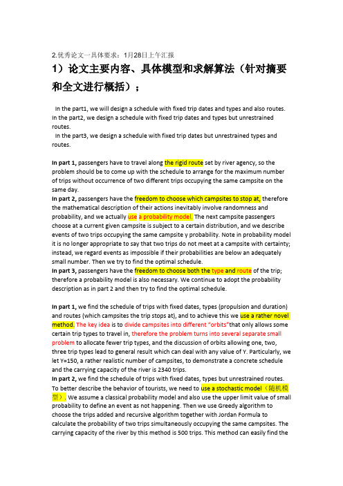
2.优秀论文一具体要求:1月28日上午汇报1)论文主要内容、具体模型和求解算法(针对摘要和全文进行概括);In the part1, we will design a schedule with fixed trip dates and types and also routes. In the part2, we design a schedule with fixed trip dates and types but unrestrained routes.In the part3, we design a schedule with fixed trip dates but unrestrained types and routes.In part 1, passengers have to travel along the rigid route set by river agency, so the problem should be to come up with the schedule to arrange for the maximum number of trips without occurrence of two different trips occupying the same campsite on the same day.In part 2, passengers have the freedom to choose which campsites to stop at, therefore the mathematical description of their actions inevitably involve randomness and probability, and we actually use a probability model. The next campsite passengers choose at a current given campsite is subject to a certain distribution, and we describe events of two trips occupying the same campsite y probability. Note in probability model it is no longer appropriate to say that two trips do not meet at a campsite with certainty; instead, we regard events as impossible if their probabilities are below an adequately small number. Then we try to find the optimal schedule.In part 3, passengers have the freedom to choose both the type and route of the trip; therefore a probability model is also necessary. We continue to adopt the probability description as in part 2 and then try to find the optimal schedule.In part 1, we find the schedule of trips with fixed dates, types (propulsion and duration) and routes (which campsites the trip stops at), and to achieve this we use a rather novel method. The key idea is to divide campsites into different “orbits”that only allows some certain trip types to travel in, therefore the problem turns into several separate small problem to allocate fewer trip types, and the discussion of orbits allowing one, two, three trip types lead to general result which can deal with any value of Y. Particularly, we let Y=150, a rather realistic number of campsites, to demonstrate a concrete schedule and the carrying capacity of the river is 2340 trips.In part 2, we find the schedule of trips with fixed dates, types but unrestrained routes. To better describe the behavior of tourists, we need to use a stochastic model(随机模型). We assume a classical probability model and also use the upper limit value of small probability to define an event as not happening. Then we use Greedy algorithm to choose the trips added and recursive algorithm together with Jordan Formula to calculate the probability of two trips simultaneously occupying the same campsites. The carrying capacity of the river by this method is 500 trips. This method can easily find theoptimal schedule with X given trips, no matter these X trips are with fixed routes or not. In part 3, we find the optimal schedule of trips with fixed dates and unrestrained types and routes. This is based on the probability model developed in part 2 and we assign the choice of trip types of the tourists with a uniform distribution to describe their freedom to choose and obtain the results similar to part 2. The carrying capacity of the river by this method is 493 trips. Also this method can easily find the optimal schedule with X given trips, no matter these X trips are with fixed routes or not.2)论文结构概述(列出提纲,分析优缺点,自己安排的结构);1 Introduction2 Definitions3 Specific formulation of problem4 Assumptions5 Part 1 Best schedule of trips with fixed dates, types and also routes.5.1 Method5.1.1 Motivation and justification5.1.2 Key ideas5.2 Development of the model5.2.1Every campsite set for every single trip type5.2.2 Every campsite set for every multiple trip types5.2.3One campsite set for all trip types6 Part 2 Best schedule of trips with fixed dates and types, but unrestrained routes.6.1 Method6.1.1 Motivation and justification6.1.2 Key ideas6.2 Development of the model6.2.1 Calculation of p(T,x,t)6.2.2 Best schedule using Greedy algorithm6.2.3 Application to situation where X trips are given7 Part 3 Best schedule of trips with fixed dates, but unrestrained types and routes.7.1 Method7.1.1 Motivation and justification7.1.2 Key ideas7.2 Development of the model8 Testing of the model----Sensitivity analysis8.1Stability with varying trip types chosen in 68.2The sensitivity analysis of the assumption 4④8.3 The sensitivity analysis of the assumption 4⑥9 Evaluation of the model9.1 Strengths and weaknesses9.1.1 Strengths9.1.2 Weakness9.2 Further discussion10 Conclusions11 References12 Letter to the river managers3)论文中出现的好词好句(做好记录);用于问题的转化We regard the carrying capacity of the river as the maximum total number of trips available each year, hence turning the task of the river managers into looking for the best schedule itself.表明我们在文中所做的工作We have examined many policies for different river…..问题的分解We mainly divide the problem into three parts and come up with three different….对我们工作的要求:Given the above considerations, we want to find the optimal。
2010数学建模优秀论文(1).doc
数学建模比赛预选赛温室中的绿色生态臭氧病虫害防治2009年12月,哥本哈根国际气候大会在丹麦举行之后,温室效应再次成为国际社会的热点。
如何有效地利用温室效应来造福人类,减少其对人类的负面影响成为全社会的聚焦点。
臭氧对植物生长具有保护与破坏双重影响,其中臭氧浓度与作用时间是关键因素,臭氧在温室中的利用属于摸索探究阶段。
假设农药锐劲特的价格为10万元/吨,锐劲特使用量10mg/kg-1水稻;肥料100元/亩;水稻种子的购买价格为5.60元/公斤,每亩土地需要水稻种子为2公斤;水稻自然产量为800公斤/亩,水稻生长自然周期为5个月;水稻出售价格为2.28元/公斤。
根据背景材料和数据,回答以下问题:(1)在自然条件下,建立病虫害与生长作物之间相互影响的数学模型;以中华稻蝗和稻纵卷叶螟两种病虫为例,分析其对水稻影响的综合作用并进行模型求解和分析。
(2)在杀虫剂作用下,建立生长作物、病虫害和杀虫剂之间作用的数学模型;以水稻为例,给出分别以水稻的产量和水稻利润为目标的模型和农药锐劲特使用方案。
(3)受绿色食品与生态种植理念的影响,在温室中引入O3型杀虫剂。
建立O3对温室植物与病虫害作用的数学模型,并建立效用评价函数。
需要考虑O3浓度、合适的使用时间与频率。
(4)通过分析臭氧在温室里扩散速度与扩散规律,设计O3在温室中的扩散方案。
可以考虑利用压力风扇、管道等辅助设备。
假设温室长50 m、宽11 m、高3.5 m,通过数值模拟给出臭氧的动态分布图,建立评价模型说明扩散方案的优劣。
(5)请分别给出在农业生产特别是水稻中杀虫剂使用策略、在温室中臭氧应用于病虫害防治的可行性分析报告,字数800-1000字。
论文题目:温室中的绿色生态臭氧病虫害防治姓名1:学号:专业:姓名1:学号:专业:姓名1:学号:专业:2010 年5月3日目录一.摘要 (4)二.问题的提出 (5)三.问题的分析 (5)四.建模过程 (6)1)问题一 (6)1.模型假设 (6)2.定义符号说明 (6)3.模型建立 (6)4.模型求解 (7)2)问题二 (9)1.基本假设 (9)2.定义符号说明 (10)3.模型建立 (10)4.模型求解 (11)3)问题三 (12)1.基本假设 (12)2.定义符号说明 (12)3.模型建立 (13)4.模型求解 (13)5.模型检验与分析 (14)6.效用评价函数 (15)7.方案 (16)4).问题四 (17)1.基本假设 (17)2.定义符号说明 (17)3.模型建立 (18)4.动态分布图 (19)5.评价方案 (19)五.模型的评价与改进 (20)六.参考文献 (21)一.摘要:“温室中的绿色生态臭氧病虫害防治”数学模型是通过臭氧来探讨如何有效地利用温室效应造福人类,减少其对人类的负面影响。
- 1、下载文档前请自行甄别文档内容的完整性,平台不提供额外的编辑、内容补充、找答案等附加服务。
- 2、"仅部分预览"的文档,不可在线预览部分如存在完整性等问题,可反馈申请退款(可完整预览的文档不适用该条件!)。
- 3、如文档侵犯您的权益,请联系客服反馈,我们会尽快为您处理(人工客服工作时间:9:00-18:30)。
Team # 10263
Page 3 of 28
3.3 Optimized Model ........................................................................................... 17 3.3.1Higher Vertical Distance ...................................................................... 17 3.3.2 Greater Degree of Twists and of Flips ................................................ 18 3.3.3 Higher Safety Coefficient .................................................................... 23 3.4 Practical Model ............................................................................................. 25 3.4.1 The Foundation of the Model.............................................................. 25 IV. Conclusions .......................................................................................................... 27 4.1 Strengths ........................................................................................................ 27 4.2 Weaknesses .................................................................................................... 27 4.3 Alternative Approaches and Future work .................................................. 27 References ................................................................................................................... 28
11.3 ~ 15.9 , and the inside surface slope angle can be set in the range 73.9 ~ 78.5 . Furthermore, computer simulation is utilized to determine
all possible landing positions so that the safe exit of the course can be properly selected. On the whole, the hemispherical course proposed has higher vertical air and stronger safety than the U-shape courses.
Байду номын сангаас
Key words: U-shape course, Hemispherical snowboard course, Height difference, Vertical angle
Team # 10263
Page 2 of 28
CONTENTS
I. Introduction .............................................................................................................. 4 1.1 Problem Restatement...................................................................................... 4 1.2 Problem Analysis ............................................................................................ 4 1.3 Some Preliminaries ......................................................................................... 5 1.4 Analysis of the Skiing Process on Current Snowboard Course (half-pipe) ................................................................................................................................. 6 1.4.1 Normal Force ......................................................................................... 7 1.4.2 Skiing Distance ...................................................................................... 8 II. Assumptions and Definitions ................................................................................. 9 2.1 Assumptions..................................................................................................... 9 2.2 Definitions ........................................................................................................ 9 III. The Models ........................................................................................................... 10 3.1 Non-air-drag Model ...................................................................................... 10 3.1.1 Terms, Definitions and Symbols .......................................................... 10 3.1.2 Additional Assumptions ....................................................................... 10 3.1.3 The Foundation of the Model.............................................................. 10 3.1.4 Model Application ................................................................................ 12 3.1.5 Analysis of the Result ........................................................................... 13 3.2 Air-drag Model.............................................................................................. 13 3.2.1 Extra Symbols ...................................................................................... 13 3.2.2 Additional Assumption ......................................................................... 14 3.2.3 The Foundation of the Model.............................................................. 14 3.2.4 Model Application ................................................................................ 15 3.2.5 Analysis of the Result ........................................................................... 16