Generation of density perturbations due to the birth of baryons

合集下载

数学专业英语词汇（T）_数学物理英语词汇

t distribution 学生t分布t number t数t statistic t统计量t test t检验t1topological space t1拓扑空间t2topological space t2拓扑空间t3topological space 分离空间t4topological space 正则拓扑空间t5 topological space 正规空间t6topological space 遗传正规空间table 表table of random numbers 随机数表table of sines 正弦表table of square roots 平方根表table of values 值表tabular 表的tabular value 表值tabulate 制表tabulation 造表tabulator 制表机tacnode 互切点tag 标签tame 驯顺嵌入tame distribution 缓增广义函数tamely imbedded 驯顺嵌入tangency 接触tangent 正切tangent bundle 切丛tangent cone 切线锥面tangent curve 正切曲线tangent function 正切tangent line 切线tangent of an angle 角的正切tangent plane 切平面tangent plane method 切面法tangent surface 切曲面tangent vector 切向量tangent vector field 切向量场tangent vector space 切向量空间tangential approximation 切线逼近tangential component 切线分量tangential curve 正切曲线tangential equation 切线方程tangential stress 切向应力tangents method 切线法tape 纸带tape inscription 纸带记录tariff 税tautology 重言taylor circle 泰勒圆taylor expansion 泰勒展开taylor formula 泰勒公式taylor series 泰勒级数technics 技术technique 技术telegraph equation 电报方程teleparallelism 绝对平行性temperature 温度tempered distribution 缓增广义函数tend 倾向tendency 瞧tension 张力tensor 张量tensor algebra 张量代数tensor analysis 张量分析tensor bundle 张量丛tensor calculus 张量演算法tensor density 张量密度tensor differential equation 张量微分方程tensor field 张量场tensor form 张量形式tensor form of the first kind 第一张量形式tensor function 张量函数tensor of torsion 挠率张量tensor product 张量乘积tensor product functor 张量乘积函子tensor representation 张量表示tensor space 张量空间tensor subspace 张量子空间tensor surface 张量曲面tensorial multiplication 张量乘法term 项term of higher degree 高次项term of higher order 高次项term of series 级数的项terminability 有限性terminable 有限的terminal decision 最后判决terminal edge 终结边terminal point 终点terminal unit 级端设备terminal vertex 悬挂点terminate 终止terminating chain 可终止的链terminating continued fraction 有尽连分数terminating decimal 有尽小数termination 终止terminology 专门名词termwise 逐项的termwise addition 逐项加法termwise differentiation 逐项微分termwise integration 逐项积分ternary 三元的ternary connective 三元联结ternary form 三元形式ternary notation 三进制记数法ternary number system 三进制数系ternary operation 三项运算ternary relation 三项关系ternary representation og numbers 三进制记数法tertiary obstruction 第三障碍tesseral harmonic 田形函数tesseral legendre function 田形函数test 检验test for additivity 加性检验test for uniform convergence 一致收敛检验test function 测试函数test of dispersion 色散检验test of goodness of fit 拟合优度检验test of hypothesis 假设检验test of independence 独立性检验test of linearity 线性检验test of normality 正规性检验test point 测试点test routine 检验程序test statistic 检验统计量tetracyclic coordinates 四圆坐标tetrad 四元组tetragon 四角形tetragonal 正方的tetrahedral 四面角tetrahedral angle 四面角tetrahedral co ordinates 四面坐标tetrahedral group 四面体群tetrahedral surface 四面曲面tetrahedroid 四面体tetrahedron 四面形tetrahedron equation 四面体方程theorem 定理theorem for damping 阻尼定理theorem of alternative 择一定理theorem of identity for power series 幂级数的一致定理theorem of implicit functions 隐函数定理theorem of mean value 平均值定理theorem of principal axes 轴定理theorem of residues 残数定理theorem of riemann roch type 黎曼洛赫型定理theorem on embedding 嵌入定理theorems for limits 极限定理theoretical curve 理论曲线theoretical model 理论模型theory of automata 自动机理论theory of cardinals 基数论theory of complex multiplication 复数乘法论theory of complexity of computations 计算的复杂性理论theory of correlation 相关论theory of differential equations 微分方程论theory of dimensions 维数论theory of elementary divisors 初等因子理论theory of elementary particles 基本粒子论theory of equations 方程论theory of errors 误差论theory of estimation 估计论theory of functions 函数论theory of games 对策论theory of hyperbolic functions 双曲函数论theory of judgment 判断论theory of numbers 数论theory of ordinals 序数论theory of perturbations 摄动理论theory of probability 概率论theory of proportions 比例论theory of relativity 相对论theory of reliability 可靠性理论theory of representations 表示论theory of sets 集论theory of sheaves 层理论theory of singularities 奇点理论theory of testing 检验论theory of time series 时间序列论theory of transversals 横断线论theory of types 类型论thermal 热的thermodynamic 热力学的thermodynamics 热力学theta function 函数theta series 级数thick 厚的thickness 厚度thin 薄的thin set 薄集third boundary condition 第三边界条件third boundary value problem 第三边界值问题third fundamental form 第三基本形式third isomorphism theorem 第三同构定理third proportional 比例第三项third root 立方根thom class 汤姆类thom complex 汤姆复形three body problem 三体问题three dimensional 三维的three dimensional space 三维空间three dimensional torus 三维环面three eighths rule 八分之三法three faced 三面的three figur 三位的three place 三位的three point problem 三点问题three series theorem 三级数定理three sheeted 三叶的three sided 三面的three sigma rule 三规则three termed 三项的three valued 三值的three valued logic 三值逻辑three valued logic calculus 三值逻辑学threshold logic 阈逻辑time interval 时程time lag 时滞time series analysis 时序分析timesharing 分时toeplitz matrix 托普利兹矩阵tolerance 容许tolerance distribution 容许分布tolerance estimation 容许估计tolerance factor 容许因子tolerance level 耐受水平tolerance limit 容许界限tolerance region 容许区域top digit 最高位数字topological 拓扑的topological abelian group 拓扑阿贝耳群topological algebra 拓扑代数topological cell 拓扑胞腔topological circle 拓扑圆topological completeness 拓扑完备性topological complex 拓扑复形topological convergence 拓扑收敛topological dimension 拓扑维topological direct sum 拓扑直和topological dynamics 拓扑动力学topological embedding 拓扑嵌入topological field 拓扑域topological group 拓扑群topological homeomorphism 拓扑同胚topological index 拓扑指数topological invariant 拓扑不变量topological limit 拓扑极限topological linear space 拓扑线性空间topological manifold 拓扑廖topological mapping 拓扑同胚topological pair 拓扑偶topological polyhedron 曲多面体topological product 拓扑积topological residue class ring 拓扑剩余类环topological ring 拓扑环topological simplex 拓扑单形topological skew field 拓扑非交换域topological space 拓扑空间topological sphere 拓扑球面topological structure 拓扑结构topological sum 拓扑和topological type 拓扑型topologically complete set 拓扑完备集topologically complete space 拓扑完备空间topologically equivalent space 拓扑等价空间topologically nilpotent element 拓扑幂零元topologically ringed space 拓扑环式空间topologically solvable group 拓扑可解群topologico differential invariant 拓扑微分不变式topologize 拓扑化topology 拓扑topology of bounded convergence 有界收敛拓扑topology of compact convergence 紧收敛拓扑topology of uniform convergence 一致收敛拓扑toroid 超环面toroidal coordinates 圆环坐标toroidal function 圆环函数torque 转矩torsion 挠率torsion coefficient 挠系数torsion form 挠率形式torsion free group 非挠群torsion group 挠群torsion module 挠模torsion of a curve 曲线的挠率torsion product 挠积torsion subgroup 挠子群torsion tensor 挠率张量torsion vector 挠向量torsionfree connection 非挠联络torsionfree module 无挠模torsionfree ring 无挠环torus 环面torus function 圆环函数torus group 环面群torusknot 环面纽结total 总和total correlation 全相关total curvature 全曲率total degree 全次数total differential 全微分total differential equation 全微分方程total error 全误差total graph 全图total image 全象total inspection 全检查total instability 全不稳定性total inverse image 全逆象total matrix algebra 全阵环total matrix ring 全阵环total order 全序total predicate 全谓词total probability 总概率total probability formula 总概率公式total regression 总回归total relation 通用关系total space 全空间total stability 全稳定性total step iteration 整步迭代法total step method 整步迭代法total stiefel whitney class 全斯蒂费尔惠特尼类total subset 全子集total sum 总和total variation 全变差totally bounded set 准紧集totally bounded space 准紧空间totally differentiable 完全可微分的totally differentiable function 完全可微函数totally disconnected 完全不连通的totally disconnected graph 完全不连通图totally disconnected groupoid 完全不连通广群totally disconnected set 完全不连通集totally disconnected space 完全不连通空间totally geodesic 全测地的totally nonnegative matrix 全非负矩阵totally ordered group 全有序群totally ordered set 线性有序集totally positive 全正的totally positive matrix 全正矩阵totally quasi ordered set 完全拟有序集totally real field 全实域totally reflexive relation 完全自反关系totally regular matrix method 完全正则矩阵法totally singular subspace 全奇异子空间totally symmetric loop 完全对称圈totally symmetric quasigroup 完全对称拟群touch 相切tournament 竞赛图trace 迹trace form 迹型trace function 迹函数trace of dyadic 并向量的迹trace of matrix 矩阵的迹trace of tensor 张量的迹tracing point 追迹点track 轨迹tractrix 曳物线trajectory 轨道transcendence 超越性transcendence basis 超越基transcendence degree 超越次数transcendency 超越性transcendental element 超越元素transcendental equation 超越方程transcendental function 超越函数transcendental integral function 超越整函数transcendental number 超越数transcendental singularity 超越奇点transcendental surface 超越曲面transfer 转移transfer function 转移函数transfinite 超限的transfinite diameter 超限直径transfinite induction 超限归纳法transfinite number 超限序数transfinite ordinal 超限序数transform 变换transformation 变换transformation equation 变换方程transformation factor 变换因子transformation formulas of the coordinates 坐标的变换公式transformation function 变换函数transformation group 变换群transformation of air mass 气团变性transformation of coordinates 坐标的变换transformation of parameter 参数变换transformation of state 状态变换transformation of the variable 变量的更换transformation rules 变换规则transformation theory 变换论transformation to principal axes 轴变换transgression 超渡transient response 瞬态响应transient stability 瞬态稳定性transient state 瞬态transient time 过渡时间transition function 转移函数transition graph 转换图transition matrix 转移矩阵transition probability 转移函数transitive closure 传递闭包transitive graph 传递图transitive group of motions 可迁运动群transitive law 可迁律transitive permutation group 可迁置换群transitive relation 传递关系transitive set 可递集transitivity 可递性transitivity laws 可迁律translatable design 可旋转试验设计translate 转移translation 平移translation curve 平移曲线translation group 平移群translation invariant 平移不变的translation invariant metric 平移不变度量translation number 殆周期translation of axes 坐标轴的平移translation operator 平移算子translation surface 平移曲面translation symmetry 平移对称translation theorem 平移定理transmission channel 传输通道transmission ratio 传输比transport problem 运输问题transportation algorithm 运输算法transportation matrix 运输矩阵transportation network 运输网络transportation problem 运输问题transpose 转置transposed inverse matrix 转置逆矩阵transposed kernel 转置核transposed map 转置映射transposed matrix 转置阵transposition 对换transversal 横截矩阵胚transversal curve 横截曲线transversal field 模截场transversal lines 截线transversality 横截性transversality condition 横截条件transverse axis 横截轴transverse surface 横截曲面trapezium 不规则四边形trapezoid 不规则四边形trapezoid formula 梯形公式trapezoid method 梯形公式traveling salesman problem 转播塞尔斯曼问题tree 树trefoil 三叶形trefoil knot 三叶形纽结trend 瞧trend line 瞧直线triad 三元组trial 试验triangle 三角形triangle axiom 三角形公理triangle condition 三角形公理triangle inequality 三角形公理triangulable 可三角剖分的triangular decomposition 三角分解triangular form 三角型triangular matrix 三角形矩阵triangular number 三角数triangular prism 三棱柱triangular pyramid 四面形triangular surface 三角曲面triangulate 分成三角形triangulation 三角剖分triaxial 三轴的triaxial ellipsoid 三维椭面trichotomy 三分法trident of newton 牛顿三叉线tridiagonal matrix 三对角线矩阵tridimensional 三维的trigammafunction 三函数trigonometric 三角的trigonometric approximation polynomial 三角近似多项式trigonometric equation 三角方程trigonometric function 三角函数trigonometric moment problem 三角矩问题trigonometric polynomial 三角多项式trigonometric series 三角级数trigonometrical interpolation 三角内插法trigonometry 三角学trihedral 三面形的trihedral angle 三面角trihedron 三面体trilateral 三边的trilinear 三线的trilinear coordinates 三线坐标trilinear form 三线性形式trinomial 三项式;三项式的trinomial equation 三项方程triplanar point 三切面重点 ?triple 三元组triple curve 三重曲线triple integral 三重积分triple point 三重点triple product 纯量三重积triple product of vectors 向量三重积triple root 三重根triple series 三重级数triple tangent 三重切线triply orthogonal system 三重正交系triply tangent 三重切线的trirectangular spherical triangle 三直角球面三角形trisecant 三度割线trisect 把...三等分trisection 三等分trisection of an angle 角的三等分trisectrix 三等分角线trivalent map 三价地图trivector 三向量trivial 平凡的trivial character 单位特贞trivial cohomology functor 平凡上同弹子trivial extension 平凡扩张trivial fibre bundle 平凡纤维丛trivial graph 平凡图trivial homogeneous ideal 平凡齐次理想trivial knot 平凡纽结trivial solution 平凡解trivial subset 平凡子集trivial topology 密着拓扑trivial valuation 平凡赋值triviality 平凡性trivialization 平凡化trochoid 摆线trochoidal 余摆线的trochoidal curve 摆线true error 真误差true formula 真公式true proposition 真命题true sign 直符号true value 真值truncated cone 截锥truncated cylinder 截柱truncated distribution 截尾分布truncated pyramid 截棱锥truncated sample 截样本truncated sequence 截序列truncation 舍位truncation error 舍位误差truncation point 舍位点truth 真值truth function 真值函项truth matrix 真值表truth set 真值集合truth symbol 真符号truth table 真值表truthvalue 真值tube 管tubular knot 管状纽结tubular neighborhood 管状邻域tubular surface 管状曲面turbulence 湍流turbulent 湍聊turing computability 图灵机可计算性turing computable 图灵机可计算的turing machine 图录机turn 转向turning point 转向点twice 再次twice differentiable function 二次可微函数twin primes 素数对twisted curve 空间曲线twisted torus 挠环面two address 二地址的two address code 二地址代码two address instruction 二地址指令two body problem 二体问题two decision problem 二判定问题two digit 二位的two dimensional 二维的two dimensional laplace transformation 二重拉普拉斯变换two dimensional normal distribution 二元正态分布two dimensional quadric 二维二次曲面two dimensional vector space 二维向量空间two fold transitive group 双重可迁群two person game 两人对策two person zero sum game 二人零和对策two phase sampling 二相抽样法two place 二位的two point distribution 二点分布two point form 两点式two sample method 二样本法two sample problem 二样本问题two sample test 双样本检验two sheet 双叶的two sided condition 双边条件two sided decomposition 双边分解two sided divisor 双边因子two sided ideal 双边理想two sided inverse 双边逆元two sided module 双边模two sided neighborhood 双侧邻域two sided surface 双侧曲面two sided test 双侧检定two stage sampling 两阶段抽样法two termed expression 二项式two valued logic 二值逻辑two valued measure 二值测度two variable matrix 双变量矩阵two way array 二向分类two way classification 二向分类twopoint boundary value problem 两点边值问题type 型type problem 类型问题typenumber 型数typical mean 典型平均。

臭氧物理计算

输入文件：#T RHF/6-31+G(D) Stable=Opt TestOzone Stability0,1OO,1,1.272O,2,1.272,1,116.8输出文件：#T RHF/6-31+G(D) Stable=Opt Test-----------------------------------------------Ozone Stability---------------Symbolic Z-matrix:Charge = 0 Multiplicity = 1OO 1 1.272O 2 1.272 1 116.8Distance matrix (angstroms):1 2 31 O 0.0000002 O 1.272000 0.0000003 O 2.166793 1.272000 0.000000Framework group C2V[C2(O),SGV(O2)]Deg. of freedom 2Standard orientation:---------------------------------------------------------------------Center Atomic Atomic Coordinates (Angstroms)Number Number Type X Y Z---------------------------------------------------------------------1 8 0 0.000000 1.083397 -0.2221702 8 0 0.000000 0.000000 0.4443403 8 0 0.000000 -1.083397 -0.222170---------------------------------------------------------------------Rotational constants (GHZ): 106.6873911 13.4595422 11.951727857 basis functions, 96 primitive gaussians, 57 cartesian basis functions12 alpha electrons 12 beta electronsnuclear repulsion energy 68.8807036279 Hartrees.NAtoms= 3 NActive= 3 NUniq= 2 SFac= 2.76D+00 NAtFMM= 60 Big=FHarris functional with IExCor= 205 diagonalized for initial guess.ExpMin= 8.45D-02 ExpMax= 5.48D+03 ExpMxC= 8.25D+02 IAcc=2 IRadAn= 4 AccDes= 0.00D+00HarFok: IExCor= 205 AccDes= 0.00D+00 IRadAn= 4 IDoV=1ScaDFX= 1.000000 1.000000 1.000000 1.000000Initial guess orbital symmetries:Occupied (A1) (B2) (A1) (A1) (B2) (A1) (B2) (A1) (B1) (A2)(B2) (A1)Virtual (B1) (A1) (A1) (B2) (B1) (A1) (B2) (B2) (A2) (A1)(A1) (B1) (B2) (A1) (B2) (A1) (A1) (B2) (B1) (B2)(A1) (A2) (B1) (B2) (A1) (A2) (B1) (A1) (B2) (A1)(B2) (A2) (B1) (A1) (B2) (A1) (B2) (B1) (A2) (A1)(B2) (A1) (A1) (B2) (A1)The electronic state of the initial guess is 1-A1.SCF Done: E(RHF) = -224.255923694 A.U. after 12 cyclesConvg = 0.4407D-08 -V/T = 2.0050S**2 = 0.0000**********************************************************************Population analysis using the SCF density.**********************************************************************Orbital symmetries:Occupied (A1) (B2) (A1) (A1) (B2) (A1) (A1) (B2) (B1) (B2)(A1) (A2)Virtual (B1) (A1) (A1) (B2) (B1) (A1) (B2) (A2) (B1) (A1)(B2) (A1) (A1) (B2) (B2) (A1) (B2) (A1) (B1) (A1)(B2) (A2) (B1) (A1) (B2) (A2) (B1) (A1) (A1) (B2)(B2) (A2) (B1) (A1) (B2) (A1) (B1) (B2) (A2) (A1)(B2) (A1) (A1) (B2) (A1)The electronic state is 1-A1.Alpha occ. eigenvalues -- -20.93754 -20.72957 -20.72951 -1.76350 -1.44168Alpha occ. eigenvalues -- -1.09742 -0.83811 -0.80473 -0.78850 -0.56768Alpha occ. eigenvalues -- -0.55671 -0.49227Alpha virt. eigenvalues -- -0.05246 0.16571 0.17766 0.17978 0.21738Alpha virt. eigenvalues -- 0.25108 0.27001 0.28193 0.29916 0.30777Alpha virt. eigenvalues -- 0.34719 0.36552 0.39788 0.43546 0.44115Alpha virt. eigenvalues -- 1.18604 1.25074 1.27328 1.29296 1.32645Alpha virt. eigenvalues -- 1.34353 1.39828 1.40179 1.41297 1.44924Alpha virt. eigenvalues -- 1.62681 1.68627 1.69884 1.76486 1.76964Alpha virt. eigenvalues -- 2.04381 2.04459 2.07563 2.10705 2.35764Alpha virt. eigenvalues -- 2.58498 2.73854 2.77367 2.86928 3.04472Alpha virt. eigenvalues -- 3.28070 3.31532 4.07728 4.38728 4.54391 Condensed to atoms (all electrons):Mulliken atomic charges:11 O -0.1624432 O 0.3248853 O -0.162443Sum of Mulliken charges= 0.00000Atomic charges with hydrogens summed into heavy atoms:11 O -0.1624432 O 0.3248853 O -0.162443Sum of Mulliken charges= 0.00000Electronic spatial extent (au): <R**2>= 111.5045Charge= 0.0000 electronsDipole moment (field-independent basis, Debye):X= 0.0000 Y= 0.0000 Z= 0.8429 Tot= 0.8429 NROrb= 57 NOA= 12 NOB= 12 NV A= 45 NVB= 45**** Warning!!: The largest alpha MO coefficient is 0.24136347D+02Orbital symmetries:Occupied (A1) (B2) (A1) (A1) (B2) (A1) (A1) (B2) (B1) (B2)(A1) (A2)Virtual (B1) (A1) (A1) (B2) (B1) (A1) (B2) (A2) (B1) (A1)(B2) (A1) (A1) (B2) (B2) (A1) (B2) (A1) (B1) (A1)(B2) (A2) (B1) (A1) (B2) (A2) (B1) (A1) (A1) (B2)(B2) (A2) (B1) (A1) (B2) (A1) (B1) (B2) (A2) (A1)(B2) (A1) (A1) (B2) (A1)24 initial guesses have been made.Iteration 1 Dimension 24 NMult 24New state 1 was old state 2Iteration 2 Dimension 48 NMult 48Iteration 3 Dimension 54 NMult 54Cease iterating as an instability has been found.*********************************************************************** Stability analysis using <AA,BB:AA,BB> singles matrix:***********************************************************************Eigenvectors of the stability matrix:Eigenvector 1: Triplet-B2 Eigenvalue=-0.211647112 -> 13 0.6830612 -> 17 0.11302Eigenvector 2: Triplet-B1 Eigenvalue=-0.01388317 -> 13 -0.1185511 -> 13 0.65960Eigenvector 3: Triplet-A2 Eigenvalue= 0.01141148 -> 13 -0.1298810 -> 13 0.6328212 -> 15 -0.1118612 -> 24 0.18654Eigenvector 4: Triplet-A1 Eigenvalue= 0.04021569 -> 13 0.683619 -> 21 -0.10643Eigenvector 5: Singlet-B1 Eigenvalue= 0.079062011 -> 13 0.68240Eigenvector 6: Singlet-A2 Eigenvalue= 0.096341510 -> 13 0.6794512 -> 24 0.11407The wavefunction has an RHF -> UHF instability.Rare condition: small coef for last iteration: 0.000D+00SCF Done: E(UHF) = -224.341434740 A.U. after 17 cyclesConvg = 0.6525D-08 -V/T = 2.0026S**2 = 0.9324Annihilation of the first spin contaminant:S**2 before annihilation 0.9324, after 0.1225QCSCF skips out because SCF is already converged.NROrb= 57 NOA= 12 NOB= 12 NV A= 45 NVB= 45 **** Warning!!: The largest alpha MO coefficient is 0.23411970D+02**** Warning!!: The largest beta MO coefficient is 0.23411970D+02Orbital symmetries:Alpha Orbitals:Occupied (A1) (?A) (?A) (B2) (B2) (B2) (?B) (B2) (B2) (?B)(B2) (B2)Virtual (?B) (B2) (B2) (B2) (?B) (B2) (B2) (?B) (B2) (?B)(B2) (B2) (B2) (B2) (B2) (B2) (B2) (?B) (B2) (B2)(B2) (?B) (B2) (B2) (?B) (?B) (?B) (B2) (B2) (B2)(?B) (B2) (?B) (B2) (B2) (B2) (?B) (B2) (?B) (B2)(B2) (B2) (?C) (?C) (?C)Beta Orbitals:Occupied (A1) (?A) (?A) (B2) (B2) (B2) (?B) (B2) (B2) (?B)(B2) (B2)Virtual (?B) (B2) (B2) (B2) (?B) (B2) (B2) (?B) (B2) (?B)(B2) (B2) (B2) (B2) (B2) (B2) (B2) (?B) (B2) (B2)(B2) (?B) (B2) (B2) (?B) (?B) (?B) (B2) (B2) (B2)(?B) (B2) (?B) (B2) (B2) (B2) (?B) (B2) (?B) (B2)(B2) (B2) (?C) (?C) (?C)12 initial guesses have been made.Iteration 1 Dimension 12 NMult 12Iteration 2 Dimension 24 NMult 24Iteration 3 Dimension 27 NMult 27Iteration 4 Dimension 30 NMult 30Iteration 5 Dimension 33 NMult 33*********************************************************************** Stability analysis using <AA,BB:AA,BB> singles matrix:*********************************************************************** Eigenvectors of the stability matrix:Excited state symmetry could not be determined.Eigenvector 1: ?Spin -?Sym Eigenvalue= 0.03620078A -> 13A -0.1347811A -> 13A 0.2109212A -> 13A -0.5972212A -> 17A 0.1296912A -> 22A -0.167668B -> 13B 0.1347811B -> 13B -0.2109212B -> 13B 0.5972212B -> 17B -0.1296912B -> 22B 0.16766The wavefunction is stable under the perturbations considered.The wavefunction is already stable.The wavefunction is already stable.********************************************************************** Population analysis using the SCF density.**********************************************************************Orbital symmetries:Alpha Orbitals:Occupied (A1) (?A) (?A) (B2) (B2) (B2) (?B) (B2) (B2) (?B)(B2) (B2)Virtual (?B) (B2) (B2) (B2) (?B) (B2) (B2) (?B) (B2) (?B)(B2) (B2) (B2) (B2) (B2) (B2) (B2) (?B) (B2) (B2)(B2) (?B) (B2) (B2) (?B) (?B) (?B) (B2) (B2) (B2)(?B) (B2) (?B) (B2) (B2) (B2) (?B) (B2) (?B) (B2)(B2) (B2) (?C) (?C) (?C)Beta Orbitals:Occupied (A1) (?A) (?A) (B2) (B2) (B2) (?B) (B2) (B2) (?B)(B2) (B2)Virtual (?B) (B2) (B2) (B2) (?B) (B2) (B2) (?B) (B2) (?B)(B2) (B2) (B2) (B2) (B2) (B2) (B2) (?B) (B2) (B2)(B2) (?B) (B2) (B2) (?B) (?B) (?B) (B2) (B2) (B2)(?B) (B2) (?B) (B2) (B2) (B2) (?B) (B2) (?B) (B2)(B2) (B2) (?C) (?C) (?C)Unable to determine electronic state: an orbital has unidentified symmetry.Alpha occ. eigenvalues -- -20.80084 -20.74413 -20.70332 -1.72528 -1.42648 Alpha occ. eigenvalues -- -1.06693 -0.82177 -0.79872 -0.77924 -0.57974 Alpha occ. eigenvalues -- -0.57745 -0.53074Alpha virt. eigenvalues -- 0.06967 0.17140 0.18093 0.18626 0.22382 Alpha virt. eigenvalues -- 0.24714 0.27212 0.28767 0.31520 0.31620 Alpha virt. eigenvalues -- 0.35236 0.37958 0.40840 0.43722 0.47906 Alpha virt. eigenvalues -- 1.20108 1.27392 1.28382 1.28543 1.34302 Alpha virt. eigenvalues -- 1.35570 1.38208 1.42662 1.45313 1.46918 Alpha virt. eigenvalues -- 1.65238 1.71747 1.72365 1.76911 1.79741 Alpha virt. eigenvalues -- 2.02221 2.02761 2.09198 2.12283 2.35839 Alpha virt. eigenvalues -- 2.61521 2.75744 2.80436 2.90174 3.06618 Alpha virt. eigenvalues -- 3.30959 3.34331 4.08920 4.38238 4.59708 Beta occ. eigenvalues -- -20.80084 -20.74413 -20.70332 -1.72528 -1.42648 Beta occ. eigenvalues -- -1.06693 -0.82177 -0.79872 -0.77924 -0.57974 Beta occ. eigenvalues -- -0.57745 -0.53074Beta virt. eigenvalues -- 0.06967 0.17140 0.18093 0.18626 0.22382 Beta virt. eigenvalues -- 0.24714 0.27212 0.28767 0.31520 0.31620 Beta virt. eigenvalues -- 0.35236 0.37958 0.40840 0.43722 0.47906 Beta virt. eigenvalues -- 1.20108 1.27392 1.28382 1.28543 1.34302 Beta virt. eigenvalues -- 1.35570 1.38208 1.42662 1.45313 1.46918 Beta virt. eigenvalues -- 1.65238 1.71747 1.72365 1.76911 1.79741 Beta virt. eigenvalues -- 2.02221 2.02761 2.09198 2.12283 2.35839 Beta virt. eigenvalues -- 2.61521 2.75744 2.80436 2.90174 3.06618 Beta virt. eigenvalues -- 3.30959 3.34331 4.08920 4.38238 4.59708 Condensed to atoms (all electrons):Mulliken atomic charges:11 O -0.0212062 O 0.0424123 O -0.021206Sum of Mulliken charges= 0.00000Atomic charges with hydrogens summed into heavy atoms:11 O -0.0212062 O 0.0424123 O -0.021206Sum of Mulliken charges= 0.00000Atomic-Atomic Spin Densities.1 2 31 O 1.042685 -0.125884 0.0000002 O -0.125884 0.000000 0.1258843 O 0.000000 0.125884 -1.042685Mulliken atomic spin densities:11 O 0.9168022 O 0.0000003 O -0.916802Sum of Mulliken spin densities= 0.00000Electronic spatial extent (au): <R**2>= 110.5628Charge= 0.0000 electronsDipole moment (field-independent basis, Debye):X= 0.0000 Y= 0.0000 Z= 0.0591 Tot= 0.0591Test job not archived.1|1|UNPC-UNK|Stability|UHF|6-31+G(d)|O3|PCUSER|20-Nov-2014|0||#T RHF/6-31+G(D) STABLE=OPT TEST||Ozone Stability||0,1|O|O,1,1.272|O,2,1.272,1,116.8||Version=x86-Win32-G03RevB.05|State=1-A1|HF=-224.3414347|S2=0.93245|S2-1=0.|S2A=0.122545|RMSD=6.525e-009|Dipole=-0.0197955,0.,0.0121783|PG=C02V [C2(O1),SGV(O2)]||@We find comfort among those who agree with us -- growth among those who don't.-- Frank A. ClarkJob cpu time: 0 days 0 hours 0 minutes 6.0 seconds.File lengths (MBytes): RWF= 16 Int= 0 D2E= 0 Chk= 7 Scr= 1Normal termination of Gaussian 03 at Thu Nov 20 16:21:43 2014.。

巴罗尼密度泛函微扰理论Baroni_DFPT

R)
R
E = E0
+
1 2
u(R)
·
∂2E ∂u(R)∂u(R
)
·
u(R
)
R,R
+···
Energy derivatives & perturbation theory
H = H0 + λivi
i
E[λ] = E0 −
fiλi
+
1 2
hij λiλj + · · ·
i
ij
Energy derivatives & perturbation theory
H = H0 + λivi
i
E[λ] = E0 −
fiλi
+
1 2
hij λiλj + · · ·
i
ij
fi
=−
∂E ∂λi
λ=0
=
− Ψ0|vi|Ψ0
Energy derivatives & perturbation theory
H = H0 + λivi
i
E[λ] = E0 −
fiλi
+
1 2
Density-functional perturbation theory
forces, response functions, phonons, and all that
Stefano Baroni
Scuola Internazionale Superiore di Studi Avanzati & DEMOCRITOS National Simulation Center Trieste - Italy

金兹堡朗道理论

Ginzburg–Landau theoryFrom Wikipedia, the free encyclopediaIn physics, Ginzburg–Landau theory, named after Vitaly Lazarevich Ginzburg and Lev Landau, is a mathematical physical theory used to describe superconductivity. In its initial form, it was postulated as a phenomenological model which could describe type-I superconductors without examining their microscopic properties. Later, a version of Ginzburg–Landau theory was derived from the Bardeen-Cooper-Schrieffer microscopic theory by Lev Gor'kov, thus showing that it also appears in some limit of microscopic theory and giving microscopic interpretation of all its parameters.Contents•1Introduction•2Simple interpretation•3Coherence length and penetration depth•4Fluctuations in the Ginzburg–Landau model•5Classification of superconductors based on Ginzburg–Landau theory•6Landau–Ginzburg theories in string theory•7See also•8References•8.1PapersIntroduction[edit]Based on Landau's previously-established theory of second-order phase transitions, Ginzburg and Landau argued that the free energy, F, of a superconductor near the superconducting transition can be expressed in terms ofa complex order parameter field, ψ, which is nonzero below a phase transition into a superconducting state and isrelated to the density of the superconducting component, although no direct interpretation of this parameter was given in the original paper. Assuming smallness of |ψ| and smallness of its gradients, the free energy has the form ofa field theory.where F n is the free energy in the normal phase, α and β in the initial argument were treated as phenomenologicalparameters, m is an effective mass, e is the charge of an electron, A is the magnetic vector potential, and is the magnetic field. By minimizing the free energy with respect to variations in the order parameter and the vector potential, one arrives at the Ginzburg–Landau equationswhere j denotes the dissipation-less electric current density and Re the real part. The first equation — which bears some similarities to the time-independent Schrödinger equation, but is principally different due to a nonlinear term —determines the order parameter, ψ. The second equation then provides the superconducting current.Simple interpretation[edit]Consider a homogeneous superconductor where there is no superconducting current and the equation for ψ simplifies to:This equation has a trivial solution: ψ = 0. This corresponds to the normal state of the superconductor, that is for temperatures above the superconducting transition temperature, T>T c.Below the superconducting transition temperature, the above equation is expected to have a non-trivial solution (that is ψ ≠ 0). Under this assumption the equation above can be rearranged into:When the right hand side of this equation is positive, there is a nonzero solution for ψ (remember that the magnitude of a complex number can be positive or zero). This can be achieved by assuming the following temperature dependence of α: α(T) = α0 (T - T c) with α0/ β > 0:•Above the superconducting transition temperature, T > T c, the expression α(T) / β is positive and the right hand side of the equation above is negative. The magnitude of a complex number must be a non-negative number, so only ψ = 0 solves the Ginzburg–Landau equation.•Below the superconducting transition temperature, T < T c, the right hand side of the equation above is positive and there is a non-trivial solution for ψ. Furthermorethat is ψ approaches zero as T gets closer to T c from below. Such a behaviour is typical for a second order phase transition.In Ginzburg–Landau theory the electrons that contribute to superconductivity were proposed to forma superfluid.[1] In this interpretation, |ψ|2 indicates the fraction of electrons that have condensed into a superfluid.[1] Coherence length and penetration depth[edit]The Ginzburg–Landau equations predicted two new characteristic lengths in a superconductor which wastermed coherence length, ξ. For T > T c (normal phase), it is given bywhile for T < T c (superconducting phase), where it is more relevant, it is given byIt sets the exponential law according to which small perturbations of density of superconducting electrons recover their equilibrium value ψ0. Thus this theory characterized all superconductors by two length scales. The second one is the penetration depth, λ. It was previously introduced by the London brothers in their London theory. Expressed in terms of the parameters of Ginzburg-Landau model it iswhere ψ0 is the equilibrium value of the order parameter in the absence of an electromagnetic field. The penetration depth sets the exponential law according to which an external magnetic field decays inside the superconductor. The original idea on the parameter "k" belongs to Landau. The ratio κ = λ/ξ is presently known asthe Ginzburg–Landau parameter. It has been proposed by Landau that Type I superconductors are those with 0 < κ< 1/√2, and Type II superconductors those with κ> 1/√2.The exponential decay of the magnetic field is equivalent with the Higgs mechanism in high-energy physics. Fluctuations in the Ginzburg–Landau model[edit]Taking into account fluctuations. For Type II superconductors, the phase transition from the normal state is of second order, as demonstrated by Dasgupta and Halperin. While for Type I superconductors it is of first order as demonstrated by Halperin, Lubensky and Ma.Classification of superconductors based on Ginzburg–Landau theory[edit]In the original paper Ginzburg and Landau observed the existence of two types of superconductors depending on the energy of the interface between the normal and superconducting states.The Meissner state breaks down when the applied magnetic field is too large. Superconductors can be divided into two classes according to how this breakdown occurs. In Type I superconductors, superconductivity is abruptly destroyed when the strength of the applied field rises above a critical value H c. Depending on the geometry of the sample, one may obtain an intermediate state[2] consisting of a baroque pattern[3] of regions of normal material carrying a magnetic field mixed with regions of superconducting material containing no field. In Type II superconductors, raising the applied field past a critical value H c1 leads to a mixed state (also known as the vortex state) in which an increasing amount of magnetic flux penetrates the material, but there remains no resistance to the flow of electric current as long as the current is not too large. At a second critical field strength H c2, superconductivity is destroyed. The mixed state is actually caused by vortices in the electronic superfluid, sometimes called fluxons because the flux carried by these vortices is quantized. Most pure elemental superconductors, except niobium and carbon nanotubes, are Type I, while almost all impure and compound superconductors are Type II.The most important finding from Ginzburg–Landau theory was made by Alexei Abrikosov in 1957. He used Ginzburg–Landau theory to explain experiments on superconducting alloys and thin films. He found that in a type-II superconductor in a high magnetic field, the field penetrates in a triangular lattice of quantized tubes offlux vortices.[citation needed]Landau–Ginzburg theories in string theory[edit]In particle physics, any quantum field theory with a unique classical vacuum state and a potential energy witha degenerate critical point is called a Landau–Ginzburg theory. The generalization to N=(2,2) supersymmetric theories in 2 spacetime dimensions was proposed by Cumrun Vafa and Nicholas Warner in the November 1988 article Catastrophes and the Classification of Conformal Theories, in this generalization one imposes thatthe superpotential possess a degenerate critical point. The same month, together with Brian Greene they argued that these theories are related by a renormalization group flow to sigma models on Calabi–Yau manifolds in thepaper Calabi–Yau Manifolds and Renormalization Group Flows. In his 1993 paper Phases of N=2 theories intwo-dimensions, Edward Witten argued that Landau–Ginzburg theories and sigma models on Calabi–Yau manifolds are different phases of the same theory. A construction of such a duality was given by relating the Gromov-Witten theory of Calabi-Yau orbifolds to FJRW theory an analogous Landau-Ginzburg "FJRW" theory in The Witten Equation, Mirror Symmetry and Quantum Singularity Theory. Witten's sigma models were later used to describe the low energy dynamics of 4-dimensional gauge theories with monopoles as well as brane constructions. Gaiotto, Gukov & Seiberg (2013)See also[edit]•Domain wall (magnetism)•Flux pinning•Gross–Pitaevskii equation•Husimi Q representation•Landau theory•Magnetic domain•Magnetic flux quantum•Reaction–diffusion systems•Quantum vortex•Topological defectReferences[edit]1.^ Jump up to:a b Ginzburg VL (July 2004). "On superconductivity and superfluidity (what I have and havenot managed to do), as well as on the 'physical minimum' at the beginning of the 21 st century". Chemphyschem.5 (7): 930–945. doi:10.1002/cphc.200400182. PMID15298379.2.Jump up^ Lev D. Landau; Evgeny M. Lifschitz (1984). Electrodynamics of Continuous Media. Course ofTheoretical Physics8. Oxford: Butterworth-Heinemann. ISBN0-7506-2634-8.3.Jump up^ David J. E. Callaway (1990). "On the remarkable structure of the superconductingintermediate state". Nuclear Physics B344 (3): 627–645. Bibcode:1990NuPhB.344..627C.doi:10.1016/0550-3213(90)90672-Z.Papers[edit]•V.L. Ginzburg and L.D. Landau, Zh. Eksp. Teor. Fiz.20, 1064 (1950). English translation in: L. D. Landau, Collected papers (Oxford: Pergamon Press, 1965) p. 546• A.A. Abrikosov, Zh. Eksp. Teor. Fiz.32, 1442 (1957) (English translation: Sov. Phys. JETP5 1174 (1957)].) Abrikosov's original paper on vortex structure of Type-II superconductors derived as a solution of G–L equations for κ > 1/√2•L.P. Gor'kov, Sov. Phys. JETP36, 1364 (1959)• A.A. Abrikosov's 2003 Nobel lecture: pdf file or video•V.L. Ginzburg's 2003 Nobel Lecture: pdf file or video•Gaiotto, David; Gukov, Sergei; Seiberg, Nathan (2013), "Surface Defects and Resolvents" (PDF), Journal of High Energy Physics。

求解RCPSP问题的迭代局部搜索算法研究

求解RCPSP问题的迭代局部搜索算法研究赵轩【摘要】Iterated Local Search algorithm is a simple and efficient metaheuristic. Presents a new iterated local search algorithm for resource-con-strained project scheduling problem (RCPSP) . Through the iterated exchange of current solution to achieve local search process, and the way of further perturbation of multiple tasks can also prevent local optimization. During the iterative process further reduces the solution space by prioritizing critical chain tasks for local search. Uses the double justification techniques to improve the quality of the solution. Uses the standard library to determine the parameters and verify the quality of the algorithm.%迭代局部搜索（Iterated Local Search）算法是一个简单、高效的元启发式算法。

提出一种新的求解资源受限项目调度问题（RCPSP）的迭代局部搜索算法。

通过对当前解进行迭代交换实现局部搜索过程，再通过扰动多个任务的方式进行有效的扰动，防止陷入局部最优。

迭代过程中通过优先对关键链的任务进行局部搜索进一步缩小解空间，通过双对齐技术提高解的质量。

机械专业毕业论文中英文翻译--在全接触条件下,盘式制动器摩擦激发瞬态热弹性不稳定的研究

Frictionally excited thermoelastic instability in disc brakes—Transientproblem in the full contact regimeAbstractExceeding the critical sliding velocity in disc brakes can cause unwanted forming of hot spots, non-uniform distribution of contact pressure, vibration, and also, in many cases, permanent damage of the disc. Consequently, in the last decade, a great deal of consideration has been given to modeling methods of thermo elastic instability (TEI), which leads to these effects. Models based on the finite element method are also being developed in addition to the analytical approach. The analytical model of TEI development described in the paper by Lee and Barber [Frictionally excited thermo elastic instability in automotive disk brakes. ASME Journal of Tribology 1993;115:607–14] has been expanded in the presented work. Specific attention was given to the modification of their model, to catch the fact that the arc length of pads is less than the circumference of the disc, and to the development of temperature perturbation amplitude in the early stage of breaking, when pads are in the full contact with the disc. A way is proposed how to take into account both of the initial non-flatness of the disc friction surface and change of the perturbation shape inside the disc in the course of braking.Keywords: Thermo elastic instability; TEI; Disc brake; Hot spots1. IntroductionFormation of hot spots as well as non-uniform distribution of the contact pressure is an unwanted effect emerging in disc brakes in the course of braking or during engagement of a transmission clutch. If the sliding velocity is high enough, this effect can become unstable and can result in disc material damage, frictional vibration, wear, etc. Therefore, a lot of experimental effort is being spent to understand better this effect (cf. Refs.) or to model it in the most feasible fashion. Barber described the thermo elastic instability (TEI)as the cause of the phenomenon. Later Dow and Burton and Burton et al.introduced a mathematical model to establish critical sliding velocity for instability, where two thermo elastic half-planes are considered in contact along their common interface. It is in a work by Lee and Barber that the effect of the thickness was considered and that a model applicable for disc brakes was proposed. Lee and Barber’s model is made up with a metallic layer sliding between twohalf-planes of frictional material. Only recently a parametric analysis of TEI in disc brakes was made or TEI in multi-disc clutches and brakes was modeled. The evolution of hot spots amplitudes has been addressed in Refs. Using analytical approach or the effect of intermittent contact was considered. Finally, the finite element method was also applied to render the onset of TEI (see Ref.).The analysis of nonlinear transient behavior in the mode, when separated contact regions occur, is even accomplished in Ref. As in the case of other engineering problems of instability, it turns out that a more accurate prediction by mathematical modeling is often questionable. This is mainly imparted by neglecting various imperfections and random fluctuations or by the impossibility to describe all possible influences appropriately. Therefore, some effort aroused to interpret results of certain experiments in addition to classical TEI (see, e.g.Ref).This paper is related to the work by Lee and Barber [7].Using an analytical approach, it treats the inception of TEI and the development of hot spots during the full contact regime in the disc brakes. The model proposed in Section 2 enables to cover finite thickness of both friction pads and the ribbed portion of the disc. Section 3 is devoted to the problems of modeling of partial disc surface contact with the pads. Section 4 introduces the term of ‘‘thermal capacity of perturbation’’ emphasizing its association with the value of growth rate, or the sliding velocity magnitude. An analysis of the disc friction surfaces non-flatness and its influence on initial amplitude of perturbations is put forward in the Section 5. Finally, the Section 6 offers a model of temperature perturbation development initiated by the mentioned initial discnon-flatness in the course of braking. The model being in use here comes from a differential equation that covers the variation of the‘‘thermal capacity’’ during the full contact regime of the braking.2. Elaboration of Lee and Barber modelThe brake disc is represented by three layers. The middle one of thickness 2a3 stands for the ribbed portion of the disc with full sidewalls of thickness a2 connected to it. The pads are represented by layers of thickness a1, which are immovable and pressed to each other by a uniform pressure p. The brake disc slips in between these pads at a constant velocity V.We will investigate the conditions under which a spatially sinusoidal perturbation in the temperature and stress fields can grow exponentially with respect to the time in a similar manner to that adopted by Lee and Barber. It is evidenced in their work [7] that it is sufficient to handle only the antisymmetric problem. The perturbations that are symmetric with respect to the midplane of the disc can grow at a velocity well above the sliding velocity V thus being made uninteresting.Let us introduce a coordinate system （x1; y1）fixed to one of the pads (see Fig. 1) thepoints of contact surface between the pad and disc having y1 = 0. Furthermore, let acoordinate system （x2; y2）be fixed to the disc with y2=0 for the points of the midplane. We suppose the perturbation to have a relative velocity ci with respect to the layer i, and the coordinate system （x; y）to move together with the perturbated field. Then we can writeV = c1 -c2; c2 = c3; x = x1 -c1t = x2 -c2t,x2 = x3; y = y2 =y3 =y1 + a2 + a3.We will search the perturbation of the uniform temperature field in the formand the perturbation of the contact pressure in the formwhere t is the time, b denotes a growth rate, subscript I refers to a layer in the model, and j =-1½is the imaginary unit. The parameter m=m（n）=2pin/cir =2pi/L, where n is the number of hot spots on the circumference of the disc cir and L is wavelength of perturbations. The symbols T0m and p0m in the above formulae denote the amplitudes of initial non-uniformities (e.g. fluctuations). Both perturbations (2) and (3) will be searched as complex functions their real part describing the actual perturbation of temperature or pressure field.Obviously, if the growth rate b<0, the initial fluctuations are damped. On the other hand, instability develops ifB〉0.2.1. Temperature field perturbationHeat flux in the direction of the x-axis is zero when the ribbed portion of the disc is considered. Next, let us denote ki = Ki/Qicpi coefficient of the layer i temperature diffusion. Parameters Ki, Qi, cpi are, respectively, the thermal conductivity, density and specific heat of the material for i =1,2. They have been re-calculated to the entire volume of the layer (i = 3) when the ribbed portion of the disc is considered. The perturbation of the temperature field is the solution of the equationsWith and it will meet the following conditions:1，The layers 1 and 2 will have the same temperature at the contact surface2，The layers 2 and 3 will reach the same temperature and the same heat flux in the direction y,3，Antisymmetric condition at the midplaneThe perturbations will be zero at the external surface of a friction pad(If, instead, zero heat flux through external surface has been specified, we obtain practically identical numerical solution for current pads).If we write the temperature development in individual layers in a suitable formwe obtainwhereand2.2. Thermo elastic stresses and displacementsFor the sake of simplicity, let us consider the ribbed portion of the disc to be isotropic environment with corrected modulus of elasticity though, actually, the stiffness of this layer in the direction x differs from that in the direction y. Such simplification is, however, admissible as the yielding central layer 3 practically does not take effect on the disc flexural rigidity unlike full sidewalls (layer 2). Given a thermal field perturbation, we can express the stress state and displacements caused by this perturbation for any layer. The thermo elastic problem can be solved by superimposing a particular solution on the general isothermal solution. We look for the particular solution of a layer in form of a strain potential. The general isothermal solution is given by means of the harmonic potentials after Green and Zerna (see Ref.[18]) and contains four coefficients A, B, C, D for every layer. The relateddisplacement and stress field components are written out in the Appendix A.在全接触条件下，盘式制动器摩擦激发瞬态热弹性不稳定的研究摘要超过临界滑动盘式制动器速度可能会导致形成局部过热，不统一的接触压力，振动分布，而且，在多数情况下，会造成盘式制动闸永久性损坏。

RCS 计算平板或圆球的手算公式

RADAR CROSS SECTION (RCS)Radar cross section is the measure of a target's ability to reflect radar signals in the direction of the radar receiver, i.e. it is a measure of the ratio of backscatter power per steradian (unit solid angle) in the direction of the radar (from the target)to the power density that is intercepted by the target.The RCS of a target can be viewed as a comparison of the strength of the reflected signal from a target to the reflected signal from a perfectly smooth sphere of cross sectional area of 1 m as shown in Figure 1 .2The conceptual definition of RCS includes the fact that not all of the radiated energy falls on the target. A target’s RCS (F ) is most easily visualized as the product of three factors:F = Projected cross section x Reflectivity x Directivity .RCS(F ) is used in Section 4-4 for an equation representing power reradiated from the target.Reflectivity: The percent of intercepted power reradiated (scattered) by the target.Directivity: The ratio of the power scattered back in the radar's direction to the power that would have been backscattered had the scattering been uniform in all directions (i.e. isotropically).Figures 2 and 3 show that RCS does not equal geometric area. For a sphere, the RCS, F = B r ,2where r is the radius of the sphere.The RCS of a sphere is independent of frequency if operating at sufficiently high frequencies where 8<<Range, and 8<< radius (r). Experimentally,radar return reflected from a target is compared to the radar return reflected from a sphere which has a frontal or projected area of one square meter (i.e.diameter of about 44 in). Using the spherical shape aids in field or laboratory measurements since orientation or positioning of the sphere will not affect radar reflection intensity measurements as a flat plate would. If calibrated, other sources (cylinder, flat plate, or corner reflector, etc.) could be used for comparative measurements.To reduce drag during tests, towed spheres of 6", 14" or 22" diameter may be used instead of the larger 44" sphere, and thereference size is 0.018, 0.099 or 0.245 m respectively instead of 1 m. When smaller sized spheres are used for tests you 2 2may be operating at or near where 8-radius. If the results are then scaled to a 1 m reference, there may be some 2perturbations due to creeping waves. See the discussion at the end of this section for further details.In Figure 4, RCS patterns are shown asobjects are rotated about their vertical axes(the arrows indicate the direction of theradar reflections).The sphere is essentially the same in alldirections.The flat plate has almost no RCS exceptwhen aligned directly toward the radar.The corner reflector has an RCS almost ashigh as the flat plate but over a wider angle,i.e., over ±60E, the return from a cornerreflector is analogous to that of a flat platealways being perpendicular to yourcollocated transmitter and receiver.Targets such as ships and aircraft oftenhave many effective corners. Corners are sometimes used as calibration targets or as decoys, i.e. corner reflectors.An aircraft target is very complex. It has a great many reflecting elements and shapes. The RCS of real aircraft must be measured. It varies significantly depending upon the direction of the illuminating radar.P r 'PtGtGr82F(4B)3R4R2 BT 'PtGtFPjGj4BP r 'PtGtGr82F(4B)3R4'PjGjGr82(4B R)288S J. Typical Aircraft RCSFigure 5 shows a typical RCS plot of a jet aircraft. The plot is anazimuth cut made at zero degrees elevation (on the aircrafthorizon). Within the normal radar range of 3-18 GHz, the radarreturn of an aircraft in a given direction will vary by a few dB asfrequency and polarization vary (the RCS may change by a factorof 2-5). It does not vary as much as the flat plate.As shown in Figure 5, the RCS is highest at the aircraft beam dueto the large physical area observed by the radar and perpendicularaspect (increasing reflectivity). The next highest RCS area is thenose/tail area, largely because of reflections off the engines orpropellers. Most self-protection jammers cover a field of view of+/- 60 degrees about the aircraft nose and tail, thus the high RCSon the beam does not have coverage. Beam coverage isfrequently not provided due to inadequate power available tocover all aircraft quadrants, and the side of an aircraft istheoretically exposed to a threat 30% of the time over the averageof all scenarios.Typical radar cross sections are as follows: Missile 0.5 sq m; Tactical Jet 5 to 100 sq m; Bomber 10 to 1000 sq m; and ships 3,000 to 1,000,000 sq m. RCS can also be expressed in decibels referenced to a square meter (dBsm) which equals 10 log (RCS in m).2Again, Figure 5 shows that these values can vary dramatically. The strongest return depicted in the example is 100 m in2 the beam, and the weakest is slightly more than 1 m in the 135E/225E positions. These RCS values can be very misleading2because other factors may affect the results. For example, phase differences, polarization, surface imperfections, and material type all greatly affect the results. In the above typical bomber example, the measured RCS may be much greater than 1000 square meters in certain circumstances (90E, 270E).SIGNIFICANCE OF THE REDUCTION OF RCSIf each of the range or power equations that have an RCS (F) term is evaluated for the significance of decreasing RCS, Figure 6 results. Therefore, an RCS reduction can increase aircraft survivability. The equations used in Figure 6 are as follows:Range (radar detection): From the 2-way range equation in Section 4-4: Therefore, R%F or F% R41/4Range (radar burn-through): The crossover equation in Section 4-8 has:Therefore, R%F or F% RBT BT21/2Power (jammer): Equating the received signal return (P) in the two way range equation to the received jammer signal (P)r r in the one way range equation, the following relationship results:Therefore, P%F or F% P Note: jammer transmission line loss is combined with the jammer antenna gain to obtain G.j j t-.46-.97-1.55-2.2-3.0-4.0-5.2-7.0-10.0-400.10.20.30.40.50.60.70.80.91.0dB REDUCTION OF RANGEdB REDUCTION OF RANGE10 Log ( P 'j / P j )(DETECTION )(BURN-THROUGH)(JAMMER)j / P jFigure 6. Reduction of RCS Affects Radar Detection, Burn-through, and Jammer PowerExample of Effects of RCS Reduction - As shown in Figure 6, if the RCS of an aircraft is reduced to 0.75 (75%) of its original value, then (1) the jammer power required to achieve the same effectiveness would be 0.75 (75%) of the original value (or -1.25 dB). Likewise, (2) If Jammer power is held constant, then burn-through range is 0.87 (87%) of its original value (-1.25 dB), and (3) the detection range of the radar for the smaller RCS target (jamming not considered) is 0.93 (93%)of its original value (-1.25 dB).OPTICAL / MIE / RAYLEIGH REGIONSFigure 7 shows the different regions applicable for computing the RCS of a sphere. The optical region (“far field”counterpart) rules apply when 2B r/8 > 10. In this region, the RCS of a sphere is independent of frequency. Here, the RCS of a sphere, F = B r . The RCS equation breaks down primarily due to creeping waves in the area where 8-2B r. This area 2is known as the Mie or resonance region. If we were using a 6" diameter sphere, this frequency would be 0.6 GHz. (Any frequency ten times higher, or above 6 GHz, would give expected results). The largest positive perturbation (point A)occurs at exactly 0.6 GHz where the RCS would be 4 times higher than the RCS computed using the optical region formula.Just slightly above 0.6 GHz a minimum occurs (point B) and the actual RCS would be 0.26 times the value calculated by using the optical region formula. If we used a one meter diameter sphere, the perturbations would occur at 95 MHz, so any frequency above 950 MHz (-1 GHz) would give predicted results.CREEPING WAVESThe initial RCS assumptions presume that we are operating in the optical region (8<<Range and 8<<radius). There is a region where specular reflected (mirrored) waves combine with back scattered creeping waves both constructively and destructively as shown in Figure 8. Creeping waves are tangential to a smooth surface and follow the "shadow" region of the body. They occur when the circumference of the sphere - 8 and typically add about 1 m to the RCS at certain 2frequencies.。

Heat transfer

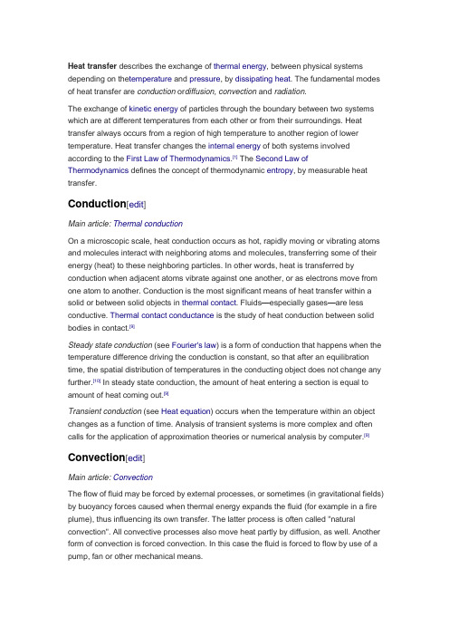
Heat transfer describes the exchange of thermal energy, between physical systems depending on the temperature and pressure, by dissipating heat. The fundamental modes of heat transfer are conduction or diffusion, convection and radiation.The exchange of kinetic energy of particles through the boundary between two systems which are at different temperatures from each other or from their surroundings. Heat transfer always occurs from a region of high temperature to another region of lower temperature. Heat transfer changes the internal energy of both systems involved according to the First Law of Thermodynamics.[1] The Second Law ofThermodynamics defines the concept of thermodynamic entropy, by measurable heat transfer.Conduction[edit]Main article: Thermal conductionOn a microscopic scale, heat conduction occurs as hot, rapidly moving or vibrating atoms and molecules interact with neighboring atoms and molecules, transferring some of their energy (heat) to these neighboring particles. In other words, heat is transferred by conduction when adjacent atoms vibrate against one another, or as electrons move from one atom to another. Conduction is the most significant means of heat transfer within a solid or between solid objects in thermal contact. Fluids—especially gases—are less conductive. Thermal contact conductance is the study of heat conduction between solid bodies in contact.[9]Steady state conduction (see Fourier's law) is a form of conduction that happens when the temperature difference driving the conduction is constant, so that after an equilibration time, the spatial distribution of temperatures in the conducting object does not change any further.[10] In steady state conduction, the amount of heat entering a section is equal to amount of heat coming out.[9]Transient conduction (see Heat equation) occurs when the temperature within an object changes as a function of time. Analysis of transient systems is more complex and often calls for the application of approximation theories or numerical analysis by computer.[9]Convection[edit]Main article: ConvectionThe flow of fluid may be forced by external processes, or sometimes (in gravitational fields) by buoyancy forces caused when thermal energy expands the fluid (for example in a fire plume), thus influencing its own transfer. The latter process is often called "natural convection". All convective processes also move heat partly by diffusion, as well. Another form of convection is forced convection. In this case the fluid is forced to flow by use of a pump, fan or other mechanical means.Convective heat transfer, or convection, is the transfer of heat from one place to another by the movement of fluids, a process that is essentially the transfer of heat via mass transfer. Bulk motion of fluid enhances heat transfer in many physical situations, such as (for example) between a solid surface and the fluid.[11] Convection is usually the dominant form of heat transfer in liquids and gases. Although sometimes discussed as a third method of heat transfer, convection is usually used to describe the combined effects of heat conduction within the fluid (diffusion) and heat transference by bulk fluid flow streaming.[12] The process of transport by fluid streaming is known as advection, but pure advection is a term that is generally associated only with mass transport in fluids, such as advection of pebbles in a river. In the case of heat transfer in fluids, where transport by advection in a fluid is always also accompanied by transport via heat diffusion (also known as heat conduction) the process of heat convection is understood to refer to the sum of heat transport by advection and diffusion/conduction.Free, or natural, convection occurs when bulk fluid motions (streams and currents) are caused by buoyancy forces that result from density variations due to variations of temperature in the fluid. Forced convection is a term used when the streams and currents in the fluid are induced by external means—such as fans, stirrers, and pumps—creating an artificially induced convection current.[13]Radiation[edit]Red-hot iron object, transferring heat to the surrounding environment primarily through thermal radiationThermal radiation occurs through a vacuum or any transparent medium (solid or fluid). It is the transfer of energy by means of photons in electromagnetic waves governed by the same laws.[14]Earth's radiation balance depends on the incoming and the outgoing thermal radiation, Earth's energy budget. Anthropogenic perturbations in the climate system, are responsible for a positive radiative forcing which reduces the net longwave radiation loss out to Space.Thermal radiation is energy emitted by matter as electromagnetic waves, due to the pool of thermal energy in all matter with a temperature above absolute zero. Thermal radiation propagates without the presence of matter through the vacuum of space.[15]Thermal radiation is a direct result of the random movements of atoms and molecules in matter. Since these atoms and molecules are composed of charged particles(protons and electrons), their movement results in the emission of electromagnetic radiation, which carries energy away from the surface.。

单词driven的是什么汉语意思份

单词driven的是什么汉语意思(三)份单词driven的是什么汉语意思 11. Makes full use of the form-driven __S Web Central environment to provide intuitive summaries and drill-downs by organization and space hierarchies.改进的表格和报告充分利用表格驱动的__S Web Central 环境，以提供直观的汇总报表和按__、空间层级结构的细分报表。

2. An inflation model that driven by rolling tachyon is investigated and its equation of density perturbations is derived.我们研究了滚动快子驱动宇宙暴涨的可能性，导出了快子暴涨下的密度扰动方程。

3. Those lockups are ending, a factor that has accelerated the decline in share prices that began last year when investors started to worry that a two-year rally that had driven prices up sixfold had put valuations too high at a time when the global economy was weakening.现在限售期已逐步__，这个因素加剧了去年年底以来的股价跌势。

此前，投资者就已经担忧，在全球经济走软的背景下，股价在两年内上涨了五倍的__股市已经估值过高。

4. Event-driven programming stresses flexibility and asynchrony as virtues, and tries to be as modeless as possible.事件驱动编程强调灵活性和美德不同步，并试图将尽可能为无模式。

GRENO题难句摘录及分析

GRENO题难句摘录及分析GRE NO题难句摘录及分析1.That se_ ratio will be favored which ma_imizes the number ofdescendantsan individual will have and hence the number of gene copies transmitted.那种性别比例能在最大程度上增加一个个体所能拥有的后代数量,并因此能在最大程度上增加所传递到后代身上去的基因复制品的数量.2.Hardys weakness derived from his apparent inability to control thecomings and goings of these divergent impulses and from his unwillingness tocultivate and sustain the energetic and risky ones.哈代的缺陷一方面缘起于他的某种明显的无能,无法控制好那结不尽相同的创作冲动的穿梭往来;另一方面缘起于他不愿意去培养和维持那些富于生机活力和风险性强的创作冲动.3.Virginia Woolfs provocative statement about her intentions in writingMrs. Dalloway has regularly been ignored by the critics,since it highlights anaspect of her literary interests very different from the traditional picture ofthe 诗性小说家所形成的传统见解大相径庭.所谓的诗性小说家,所关注的是审视想入非非和白日梦幻的诸般状态,并致力于追寻个体意识的通幽曲径.4.Although Gutman admits that forced separation by sale was frequent,heshows that the slavespreference,revealed most clearly on plantations where salewas infrequent,was very much for stable monogamy.虽然古特曼承认,由于奴隶买卖而造成的被迫离散甚为频繁,但他还是证明,奴隶的偏爱在那些奴隶买卖并不频繁的种植园上被最为显著地揭示出来在很大程度上侧重于稳定的一夫一妻制.5.Gutman argues convincingly that the stability of the Black family encouraged the transmission of-and so was crucial in sustaining-the Blackheritage of folklore,music,and religious e_pression from one generation toanother,a heritage that slaves were continually fashioning out of their Africanandd American e_periences.古特曼人令人信服地论辨道,黑人家庭的稳定有助于包括民间传说.音乐.及宗教表达在内的黑人文化遗产一代一代传递下去,因而在维持文化遗产方面也起着至关重要的作用,而对于这种文化遗产,黑奴们不断地从其非洲和美洲的经历中予以丰富发展.6.This preference for e_ogamy,Gutman suggests,may have derived fromWestAfrican rules governing marriage,which,though they differed from one tribalgroup to another,all involved some kind of prohibition against unions with closekin.古特曼表示,这种对于外部通婚的偏爱很有可能缘起于西部非洲制约着婚姻的规定,尽管这些规定在一个和另一个部落群体之间不尽相同,但都涉及到某种对近亲联姻的禁止.8. Such variations in size,shape,chemistry,conduction speed,e_citationthreshold,and the like as had been demonstrated in nerve cells remainednegligible in significance for any possible correlation with the manifolddimensions of mental e_perience.9.Although qualitative variance among nerve energies was never rigidlydisproved,the trine was generally abandoned in favor of the opposingview,namely,that nerve impulses are essentially homogeneous in quality and aretransmitted as common currency throughout the nervous system. Othere_perimentsrevealed slight variations in the size,number,arrangement,and interconnection ofthe nerve cells,but as far as psychoneural correlations were concerned,theobvious similarities of these sensory fields to each other seemed much moreremarkable than any of the minute differences. Although some e_periments showthat,as an object becomes familiar,its internal representation becomes moreholistic and the recognition process correspondingly more parallel,the weight ofevidence seems to support the serial hypothesis,at least for objects that arenot notably simple and familiar.虽然某些实验表明,随着一个物体变得熟悉起来,其内心再现图像亦更具整体感,辨认过程相应地更趋于平行,但证据的砝码似乎在支持序列假设,至少是对于那些不甚简单.不甚熟悉的物体来说.10.In large part as a consequence of the feminist movement,historians havefocused a great deal of attention in recent years on determining more accuratelythe status of women in various periods.在很大程度上,由于女权主义运动的缘故,史学家近年来汇聚了大量的注意力,来更为准确地确定妇女在各个历史时期的地位.GRE NO题难句摘录及分析_.Thus,for instance,it may come as a shock to mathematicians to learn thatthe Schrodinger equation for the hydrogen atom is not a literally correctdescription of this atom,but only an appro_imation to a somewhat more correctequation taking account of spin,magnetic dipole,and relativistic effects;andthat this corrected equation is itself only an imperfect appro_imation to aninfinite set of quantum field- theoretical equations.因此,举例来说,对数学家而言,了解到下述情形可能会令其惊愕不已,即薛定谔的氢原子方程式并非是对该原子作出的一种绝然正确的描述,而仅仅是个近似值,趋近于一个在某种程度上更为正确的将自旋.磁性偶极子.以及相对论效应考虑在内的方程式;而这个得以纠正的方程式就其本身而言也只是一个不完美的近似值,趋近于无穷无尽的一整套量子场论方程式._.The physicist rightly dreads precise argument,since an argument that isconvincing only if it is precise loses all its force if the assumptions on whichit is based are slightly changed,whereas an argument that is convincing thoughimprecise may well be stable under small perturbations of its underlyingassumptions.物理学家恐惧于那些精确无误的论据不无道理,因为某种只有在它是精确无误的条件下才令人置信的论据,一旦它赖于建立其上的假设稍有变化,便会失去它一部的作用;而与此相反,一个尽管并不精确无误但却令人置信的论据,在其基本假设稍微受干扰的情况下,仍然有可能是站得住脚的._.However,as they gained cohesion,the Bluestockings came to regardthemselves as a womens group and to possess a sense of female solidarity lackingin the salonnieres,who remained isolated from one another by the primacy eachheld in her own salon.起初,蓝袜女们确实模仿了法国沙龙女主人,将男性襄括到其小圈子中来.然则,随着她们获得的凝聚力,她们渐趋将自己视作一女性团体,并拥有了一种妇女团结意识,而这种意识在法国沙龙女主人身上则荡然无存,因为她们每个人在其自己的沙龙中自视甚高而彼此孤立隔绝开来._.As my own studies have advanced,I have been increasingly impressed withthe functional similarities between insect and vertebrate societies and less sowith the structural differences that seem,at first glance,to constitute such animmense gulf between them.随着我的研究不断深入,我对昆虫和脊椎动物群落之间的功能类似性印象愈来愈深刻,而对结构上的差异印象愈发淡漠,虽然这些结构上的差异初看上去似乎构成了二者间一条无法愈越的鸿沟._. Although fiction assuredly springs from political circumstances,itsauthors react to those circumstances in ways other than ideological,and talkingabout novels and stories primarily as instruments of ideology circumvents muchof the fictional enterprise.虽然小说无疑起源于政治情状,但其作者则是以非意识形态的方式对这些政治情状作出反应的,而将小说和故事主要地当作意识形态的工具来探讨,会在相当程度上阻碍小说事业.GRE NO题难句摘录及分析_.Is this a defect,or are the authors working out of,or trying to forge,adifferent kind of aesthetic?这究竟是一种缺陷呢,或者是否表明,这些作者是在按照一种与众不同的美学体系进行创作,抑或是在试图创立一种与众不同的美学体系?_.Black Fiction surveys a wide variety of novels,bringing to our attentionin the process some fascinating and little-known works like James WeldonJohnsons Autobiography of an E_- Colored Man.《黑人小说》考察了极为广泛的一系列小说,在此过程中让我们注意到了某些引人入胜但却鲜为人知的作品,如詹姆斯.韦尔登.约翰逊的《一个曾经是有色人的自传》._.Although these molecules allow radiation at visible wavelengths,wheremost of the energy of sunlight is concentrated,to pass through,they absorb someof the longer-wavelength,infrared emissions radiated from the Earthssurface,radiation that would otherwise be transmitted back into space.虽然这些分子允许可见波长的辐射自然表露的情感.思维.以及行动方式.20.A low number of algal cells in the presence of a high number of grazerssuggested,but did not prove,that the grazers had removed most of the algae.在存在大量食草动物的同时却只有少量的水藻花粉囊,这暗示出但没能证明食草动物已吞噬了大部分水藻._.Studies by Hargrave and Geen estimated natural community graz-ing ratesby measuring feeding rates of individual zooplankton species in the laboratoryand then computing community grazing rates for field conditions using theknownpopulation density of grazers.由哈格雷夫和吉恩所进行的研究,对自然条件下的群落食草比例进行了估计,其手段是通过测量出实验室内单独的浮游动物种类的结食比例,然后利用已知的食草动物种群密度,计算出实地状况下的群落食草比例._.In the periods of peak zooplankton abundance,that is,in the late springand in the summer,Haney recorded ma_imum daily com-munity grazing rates,fornutrient-poor lakes and bog lakes,respectively,of 6.6 percent and _4 percent ofdaily phytoplankton production.在浮游动物数量激增的高峰期,亦即在春季后期以及夏季,哈尼记录了最大程度上的每日群落食草比率,对于营养物不充足的湖和沼泽湖而言,分别为每日浮游植物繁殖量的6.6%和_4%.23.The hydrologic cycle,a major topic in this science,is the complete cycleof phenomena through which water passes,beginning as atmospheric watervapor,passing into liquid and solid form as precipitation,thence along and intothe ground surface,and finally again returning to the form of atmospheric watervapor by means of evaporation and transpiration.水文循环,作为该学科中的一个主要课题,指的是水所经过的诸现象的整个循环过程,开始时是作为大气中的水蒸气,转而作为雨.雪.露.雹一类的降水量经过液体和固体形态,由此而沿着地层表面分布或进入地层表面,最终通过蒸发和散发作用再度回复到大气水蒸气的形态.24.The historian Frederick J. Turner wrote in the _90s that the agrariandiscontent that had been developing steadily in the United States since about_70 had been precipitated by the closing of the internalfrontiers,historianswho studied preindustrial Europe began,for the first time in large numbers,toinvestigate more of the preindustrial European population than the 2or3 percentwho comprised the political and social elite:thekings,generals,judges,nobles,bishops,and local magnates who had hitherto usuallyfilled history books.二十世纪五十年代早期,研究前工业化时代欧洲的史学家,首次以众多的人数,开始调查前工业化时代欧洲人口中的大多数,而非那些构成了政治与社会精英阶层的百分之二或三的人口,即国王.将军.法官.贵族.主教.以及地方上的达官显贵,而正是这部分人一直到那时为止普遍充斥于史学著作.GRE NO题难句摘录及分析26.Historians such as Le Roy Ladurie have used the uments to e_tractcase histories,which have illuminated the attitudes of different social groupsand have revealed how the authorities administered justice.象勒罗伊·拉迪里一类的史学家利用这些文献史料从中挖掘出某些个案史来,阐明了不同社会群体的态度,并揭示出当局是如何执行审判的.27.My point is that its central consciousnesss livesowes much to thatearlier literary heritage,a heritage that,in general,has not been sufficientlyvalued by most contemporary literary critics.我的论点是,其作品的中心意识它将阶级和性别作为人们生活的决定性影响而作出的深邃理解在很大程度上借鉴了那个早期的文学遗产,而这一遗产就总体而言还尚未获得大多数当代文学评论家的足够重视.28.But achieving necessary matches in physical properties across interfacesbetween living and nonliving matter requires knowledge of which moleculescontrol the bonding of cells to each othernaturalconstitution:specifically,theidea of inserting into nonleguminous plants the genes,if they can be identifiedand isolated,that fit the leguminous plants to be hosts for nitrogen-fi_ingbacteria. Hence,the intensified research on legumes.这其中的一个新颖思想就是,在植物的染色体内注入并非是该植物自然构造一个部分的那些不相关联的因基:具体而言,这一思想是,在非豆科植物内注入这样一些基因,倘若这些基因可被辨识出来并被分离开来,而这些基因业已使豆科植物宜于充当那些具备固氮作用的细菌的寄主.由此,对豆科植物的研究日趋深入.33.It is one of natures great ironies that the availability of nitrogen inthe soil frequently sets an upper limit on plant growth even though theplantsleaves are bathed in a sea of nitrogen gas.下述情形真可谓是自然界的一个莫大讽刺:土壤中所能获得的氮肥量往往对植物的生长构成了一个上限,虽然植物的叶子被沐浴在一片氮气的海洋中.34.Unless they succeed,the yield gains of the Green Revolution will belargely lost even if the genes in legumes that equip those plants to enter intoa symbiosis with nitrogen fi_ers are identified and isolated,and even if thetransfer of those gene comple_es,once they are found,becomes possible.除非他们能取得成功,不然的话,绿色革命的产量收益将在很大程度上损失殆尽,即使豆科植物中使这些植物有条件进入到与固氮细菌共生关系的基因可被辨识出来和分离开来的话,且即使这些基因综合体,一旦被发现之后,其移植得以成为可能的话.GRE NO题难句摘录及分析。

Density distributions

Probability Theory in Linguistics2LSA,January3,2003EXEMPLAR THEORYJanet PierrehumbertNorthwestern University1Density distributionsReview of the concept of a density distribution,as an encoding of events in the physical world.Examples in the presentation were the density of galaxies in the night sky and the death rate during the cholera epi-demic in Victorian London.Theﬁgures used at the LSA are copyrighted to T ufte(1983,1997).As T ufte claims,detailed representations are argued to be ad-vantageous.2Phonetic density distributions are acquired They differ across languages,dialects,and so-ciostylistic registers.They are learned over a long time.They are updated through experience.3Learning and updatingThe location and sharpness of the/r/-/w/bound-ary improves gradually in3to5year old children.(Slawinski and Fitzgerald,1997).Similar results for4other minimal contrasts in children aged6to12(Hazan and Barrett,2000).Fluent bilingual speaker residing in Brazil and US shortens VOTs in both unaspirated(Portuguese) and aspirated(English)stops while in Brazil.(Sancier and Fowler,1997).4Value-added categorizationProvides handles on phonetic distributions.It does not throw phonetic information away.5Why?Subphonemic details are used for other purposes.Identical twins can be distinguished by their speech.(Johnson and Azara).Phonetic details reﬂect core vs.fringe position in Latina gangs.(Mendoza-Denton).Sexual identity is effectively cued by speech.(Bent et al.,and others)6Distribution shapes must be retained because: They are typically non-Gaussian(c.f Duarte,et al.)They are important for modeling perception and production.They are used to initiate new categories bottom-up.(Maye2000,Maye and Gerken2002).7Exemplar theoryLevels:Cognitive bels/functions.Areas of map are associated with la-bels/functions.Density distributions acquired by encoding and storing experiences.Each new stimulus encoded as a location on the map.New stimuli categorized on the basis of most simi-larity to the most exemplars near that location(c.f.R.D.Luce,Kruschke)8Plausibility?Mathematical schema involves remembering every-thing:See Kruschke,Nosofsky,K.Johnson.Related neural model achieves data compression: See Guenther and Gjaja(1996)and later articles.9Production(Pierrehumbert2001,2002)Select a category to be produced.T ake a random selection from the exemplar cloud for that category.Entrenchment:Average the n neighbors of that selection to get a production target.Produce the target with some random error.1050100150200250300-1-0.500.51 1.52No Lenition or entrenchmentPhonetic characterM e m o r y -w e i g h t e d c o u n tThe Perception-production loopEvolution of distributions in a uniform population of speakers can be modeled by producing random to-kens and then”perceiving”them,e.g.running the per-ception and production models in a loop.11Critical parametersProduction:Noise versus entrenchment.Bias terms related to phonetic pressures. Perception/Memory:Encoding limits.Memory decay time.Attentional weighting(see K.Johnson,1997).12ExampleCollapse of a marked with an unmarked category.Marked category is less frequent.It is produced with a persistent bias towards the unmarked category.1350100150200-1-0.500.51 1.52Phonetic characterM e m o r y -w e i g h t e d c o u n t50100150200250300350400-1-0.500.51 1.52Phonetic characterM e m o r y -w e i g h t e d c o u n t50100150200250300350400-1-0.500.51 1.52Phonetic characterM e m o r y -w e i g h t e d c o u n t100200300400500-1-0.500.51 1.52Phonetic character M e m o r y -w e i g h t e d c o u n tExampleUnstable resolution of crowding in the phonetic space.14Evolution of five crowded categories in a2D space. Circular noise.30,000iterations.OUTCOME1:Upper left and lower right categories dominate.Same conditions.OUTCOME2:Central and lower right categories dominate.DIRECTIONMulti-agent models.Conditions for convergence(Cucker and Smale, Liberman).T ypology of outcomes and language variation(de Boers;using prototypes not full distributions).T rajectory of phonetic acquisition.15ReferencesBent,T.Janet Pierrehumbert and Michael Bailey (2002)The acoustics of lesbian vowels and the perception of women’s sexual orientation.Paper presented at McWOP8,Indiana University,Oct 25and26,2002.Cucker,F.and Smale,S.(2002)On the Mathe-matical Foundations of Learning.Bulletin of the American Mathematical Society,39(1).de Boer,Bart(2000)Self organization in vowel systems,Journal of Phonetics28(4),pp.441465 http://arti.vub.ac.be/Duarte,Galves,Garcia,Maronna.The statistical analysis of acoustic correlates of speech rhythm.p.br/tycho16Guenther and Gjaja(1996)The perceptual mag-net effect as an emergent property of neural map formation,J.Acoust.Soc.Am.100,1111-1121.See also additional papers at /guenther/.Hazan,V.and Barrett.S.(2000)The develop-ment of phonemic categorization in children aged 6-12.Journal of Phonetics28,377-397.Johnson and Azara(in press)The Percep-tion of Personal Identity in Speech:Evidence from the perception of twin’s speech.Down-load from /kjohn-son/research.htmlJohnson,K.(1997)Speech Perception without Speaker Normalization:An Exemplar Model.inK.Johnson and J.Mullenix,eds.T alker variabil-ity in speech processing,Academic Press,San Diego,145-166.Kruschke(1992)ALCOVE:An Exemplar-Based Connectionist Model of Category Learning,Psy-chological Review,99,22-44.Liberman,M.(2002)Simple Models for Emer-gence of a Shared Vocabulary,Paper de-livered at Labphon8,Y ale University,June 27-30,2002.Slides downloadable from /myl/labphon.ppt.Luce,R.D.,Bush,R.R.,Galanter,E.(1963) Handbook of Mathematical Psychology Vol.1. Maye,J.and L.Gerken(2000)Learning Phonemes Without Minimal Pairs,Proceedings ofthe24th Annual Boston University Conference on Language Development.Maye,J.and J.F.Werker and L.Gerken”(2002) Infant Sensitivity to Distributional Information Can Affect Phonetic Discrimination,Cognition,82, B101-B111.Mendoza-Denton.N(1997)Chicana/Mexicana Identity and Linguistic Variation:An Ethnographic and Sociolinguistic Study of Gang Afﬁliation in an Unrban High School.Ph.D dissertation,Stanford University.Nosofsky,R.M.(1986)Attention,Similarity, and the Identiﬁcation-categorization relationship. Journal of Experimental Psychology:Gen-eral.115,39-57.Pierrehumbert,J.(2001)Exemplar Dynam-ics:Word Frequency,Lenition and Contrast, in J.Bybee and P.Hopper,eds,Frequency Effects and Emergent Grammar,Amsterdam, John Benjamins,137-157,Downloadable from /jbp.Pierrehumbert,J.(2002)Word-speciﬁc pho-netics.in C.Gussenhoven and N.Warner, boratory Phonology VII,Mouton De Gruyter,Berlin,101-140.Downloadable from /jbp.Sancier,M.L.and Fowler,C.A.(1997)Gestural drift in bilingual speaker of Brazilian Portuguese and English.Journal of Phonetics25,421-436. Smale,S.(2002)Learning Theory and the Evolution of Language.De-partment of Computer Science Distin-guished Colloquium,University of Chicago./pipermail/visitors/2002-May/000084.htmlSlawinski,E.G.and Fitzgerald,L.K(1998)Per-ceptual development of the categorization of the /r-w/contrast in normal children.Journal of Pho-netics26,27-44.T ufte,E.R.(1997)Visual Explanations.Graphics Press,Cheshire CN.T ufte,E.R.(1983)The Visual Display of Quanti-tative Information.Graphics Press,Cheshire CN.。

RCS 计算平板或圆球的手算公式

卫星轨道外推：第二部分(英文批注)

Orbital Propagation: Part II轨道外推：第二部分By Dr. T.S. KelsoIn our last column, we covered the basics of modeling as they apply to predicting the position of a satellite in earth orbit. As with any model, the complexity of the orbital model we choose depends upon several factors, chief among these being the accuracy of the desired predictions. At the same time, since we will be calculating predictions from this orbital model on a computer, we would also like to reduce the computational complexity of the model. Unfortunately, these two goals conflict, so we will seek a model which strikes an appropriate balance between the model's fidelity (accuracy) and the computational burden of producing a prediction.In order to obtain the appropriate level of model fidelity, it will be necessary to determine the types and relative magnitudes of the forces acting upon the satellite. For our orbital model, these include the gravity of the earth along with perturbations due to the nonuniform mass distribution of the earth, gravitational attraction of the sun, moon, and planets, and atmospheric drag. Which of these forces are most important will depend not only on their relative magnitude but upon whether their effects are periodic or secular.A periodic effect, such as your car's antenna whipping back and forth as you drive down the road, has little effect on the position of the tip of the antenna over time, even though the forces involved may be rather large. If you only need to know the position of the antenna tip to within one meter, you will likely ignore this effect. However, a secular effect, one which consistently increases or decreases over time, may have a considerable effect even though the force involved may be small. An example of a secular effect would be that of a light wind blowing a sailboat across the water.As far as computational complexity is concerned, we noted at the close of the last column that there were two primary computational methods of implementing an orbital model. One was to start with a satellite's position and velocity and to sum, or integrate, all of the forces acting on the satellite. This total force is assumed to act on the satellite over some small time span, at the end of which a new position and velocity is calculated and the process is repeated. When implemented on a computer, this approach is known as numerical integration. The advantage of this approach is that if sufficient detail is given to the forces acting upon the satellite and small enough time steps are used, highly-accurate predictions can be obtained. The down side to numerical integration is that we must calculate the satellite's position and velocity for each time step between our known initial conditions and our desired prediction time.Depending upon the size of the time step and the length of the time interval, the computational burden for even a single satellite can be large. Now, multiply this problem by the approximately 7,500 objects currently tracked by NORAD (the North American Aerospace Defense Command) and you'll begin to appreciate the need for another solution. We would prefer to have a model which provides an analytical solution, that is, a solution wherein if we know the time of interestwe can directly calculate the state of the satellite's orbit at that time without the need to 'step' along in time. This is our second computational method of implementing an orbital model.During the 1970s, NORAD came up with just such a solution: a fully-analytical orbital model. With this model, known as SGP (for Simplified General Perturbation), a user can calculate a satellite's position and velocity at a particular time directly, without the need for numerical integration. The result is a considerable reduction in computational burden to support tracking the growing population of earth-orbiting satellites.Obviously, some tradeoffs had to be made in the process of developing SGP. As with any model, certain simplifications had to be made and these simplifications place restrictions upon how the model can be used. In particular, the mass of the satellite relative to the mass of the earth is assumed to be negligible. In addition, the satellite is assumed to be in a low-eccentricity, near-earth orbit and not in a rapidly-decaying orbit. These conditions were true for a large percentage of the satellite population at the time SGP was developed and allowed a model to be formulated accounting only for the primary perturbations on these satellites due to the earth's nonuniform mass distribution and atmospheric drag.Subsequent refinements to SGP extended this theory to include a semi-analytic treatment of orbits with periods greater than 225 minutes. While this theory does depend to some extent upon numerical integration, the computational burden is still considerably reduced. The break at 225 minutes (about 6,000 km altitude) is the result of a somewhat natural gap which has resulted from historical choices of orbits for various satellite missions and a crossover in significant perturbing effects; above the gap the primary perturbing forces are no longer atmospheric drag and the earth's nonuniform density, but orbital resonances with the earth's nonuniform gravitational field, solar and lunar gravitational forces, and solar radiation pressure. This new model is referred to as SGP4 and is the model currently in use by NORAD and the United Stated Space Command.You may be wondering, at this point, why I am focusing on the history of SGP4. Certainly, there are many other models, many of which are more accurate than SGP4. But SGP4 has one thing going for it that none of the others do: data. Not unlike the advent of automobiles running on unleaded gasoline, it didn't make any difference how slick a new car you had if you couldn't find any unleaded gas. Most other orbital models only provide data for a limited number of satellites (such as the space shuttle). NORAD, on the other hand, is responsible for tracking all satellites on a daily basis and it uses SGP4 to do that. This means that orbital data for this model is available for all earth-orbiting objects capable of being tracked by the US Space Surveillance Network.But we're not talking about unleaded versus regular gasoline here. Aren't all orbital element sets alike? After all, they all measure things like inclination and semi-major axis (terms we'll define further in a future column) or I can convert to these terms. Why can't I take the NORAD elements and use them in my favorite tracking program (which doesn't use the SGP4 model)? Allow me to use a computer analogy here to explain.Most of you are familiar with various algorithms for compressing data. Whether you know them by their formal names, such as run-length encoding, Huffman or LZW compression, or by the terms used by some of the popular archiving packages, such as squeezing, imploding, crushing, or the like, you wouldn't be too happy with the result if someone sent you data compressed by one method and you used another to uncompress it. Of course, your software would probably report an error, but that's not true of orbital software. But the result will be the same: errors.The two-line orbital element sets made available by NORAD (and redistributed by NASA) are mean Keplerian orbital element sets. The mean values for each element are generated using the SGP4 orbital model. The effects of the major perturbing forces are incorporated into these mean values in a very specific way using SGP4 and SGP4 must be used to generate accurate predictions. Failure to do so will result in errors, the magnitude of which will depend heavily on the type of orbit being modeled. These errors are typically manifested as large time errors in satellite signal or visual acquisition or being unable to locate the satellite at all.The implications of the last couple of paragraphs should be clear. Just as you wouldn't expect to find a program compressed with LHARC to be distributed with a .ZIP extension, the only data distributed in the two-line format should be NORAD-generated SGP4-compatible data. Data from other sources should never be reformatted into the two-line format just so it can be fed into a particular software package unless you don't care about the accuracy of the results (just as you wouldn't rename a file with an .LHA extension to .ZIP just so you could use PKUNZIP).Many popular commercial, shareware, and public domain satellite tracking packages implement SGP4 and you should check for this feature if you are concerned about accurate predictions. We will review some of these packages in a future column. And, if you are concerned about the source of your data, allow me to suggest two reliable sources. Daily updates of NORAD-generated two-line orbital element sets are available via Internet (anonymous ftp, gopher, or mosaic) on in the directory pub/space or on the Celestial BBS at 205/409-9280 [Neither of these services is currently available. Data can now be found only on the CelesTrak WWW site.]. Both services are available free of charge to all users.In our next column, we will explore how the NORAD two-line element sets are generated and give some numerical examples to illustrate the magnitude of the errors which can result from improper combinations of models and data. I look forward to seeing you here next time!。

Lead paragraph

When dissipative particles are left alone, their uctuation energy decays due to collisional interactions, clusters build up and grow with time until the system size is reached. When the e ective dissipation is strong enough, this may lead to the \inelastic collapse", i.e. the divergence of the collision frequency of some particles. The cluster growth is an interesting physical phenomenon, whereas the inelastic collapse is an intrinsic e ect of the inelastic hard sphere (IHS) model used to study the cluster growth { involving only a negligible number of particles in the system. Here, we extend the IHS model by introducing an elastic contact energy and the related contact duration tc . This avoids the inelastic collapse and allows to examine the long-time behavior of the system. For a quantitative description of the cluster growth, we propose a burning{like algorithm in continuous space, that readily identi es all particles that belong to the same cluster. The criterion for this is here chosen to be only the particle distance. With this method we identify three regimes of behavior. First, for short times a homogeneous cooling state (HCS) exists, where a mean- eld theory works nicely, and the clusters are tiny and grow very slowly. Second, at a certain time which depends on the system's properties, cluster growth starts and the clusters increase in size and mass until, in the third regime, the system size is reached and most of the particles are collected in one huge cluster.

开关电源术语

计算机与网络算法与理论C++程序设计Matlab应用信息处理与优化VB、JAVA等C#技术数模电基础控制技术单片机技术DSP技术总线技术EDA软件电力电子CPLD和FPGA串口通讯相关嵌入式系统显示与光电CADCAM专业英语英语口语科技新闻思考与休闲栏目树形导航| 首页 | 文章中心 | 下载中心 | 本站特供 | 软硬件结合论坛 ||文章中心首页|软件技术|硬件技术|软硬件结合|机械相关|数理化基础|英语学习|休闲一刻|您现在的位置：中国软硬件结合技术网 >> 文章中心 >> 硬件技术 >> 电力电子 >> 正文用户登录新用户注册开关电源术语【字体：小大】开关电源术语作者：未知文章来源：未知点击数：168 更新时间：2007-11-21这些定义应被认为是有关于开关电源的，并不一定等同的适用于其它技术领域。

考虑到在其它出版物（标准，词典，制造商数据手册，技术笔记，手册）已经同时给出了定义，下列的术语仅代表作者本人的观点，并可能与使用本文档的特定用户有轻微的差别。

绝对额定最大值，元件：如果超过将导致永久性的器件损坏的规定值。

这不是连续额定值，并不表示适当的操作。

A e, 有效区域：对于给定几何尺寸的磁芯，是指具有同样磁性的同种原料的圆柱形磁芯的横截面积。

周围温度Ambient Temperature (1):目标温度和SMPS周围静止空气的温度，在距离电源最小为4" (100mm)处测得。

周围温度Ambient Temperature (2):根据MIL-STD-810E: 除了必要的支撑点，测试单元应完全出于空气的包围中。

周围空气的温度梯度应为测量温度的2℃之内且不超过1℃每米。

安培匝数Ampere Turns (NI):流过线圈的电流与线圈匝数的乘积。

ATP:验收测试步骤（Acceptance Test Procedure）。

BABT:英国无线电通讯认证部（The British Approvals Board for Telecommunications）。

专业术语及xx面板公司内的惯用缩写词组整理

BTN LCD BOM
CF CF CT
CV COA CCD CP CP Co/CO CAD CAT Cat-CVD CATV CBB CBE CCF CCFL/CFL CD CDA CD CCM CD-ROW CDT CES CEL CFF CFP CG
Air Simulation Black matrix BC Recipe Management brightness enhancement film buffered hydrofluoric acid bistable nematic blocking layer bipotential focus broadcasting statellite ballistic electron surface-emitting device bistable twisted nematic LCD Bill of Material
英文简写
英文全称
中文解释
A/K AA AC AC PDP
ACF ACP AD ADS AFLC AFLCD AFP AG AGA AGV AI AL ALE ALIS AM AM LCD AM LED AMHS AOI AOI APC APR APT AR AR
ARG ARHS a-Si TFT LCD ASIC ASM ASV ATE AUO AV AWD AP
黑色矩阵；制作黑色矩阵的制程 BC Recipe 管理（系统）增亮膜，增辉膜缓冲氢氟酸双稳态扭曲向列液晶阻隔层双电位透镜聚焦广播用卫星弹道电子表面发射器件
双稳态扭曲向列相 LCD 物料清单，是计算机可以识别的产品结构数据文件，也是 ERP 的主导文件。BOM 使系统识别产品结构，也是联系与沟通企业各项业务的纽带。ERP 系统中的 BOM 的种类主要包括 5 类：缩排式 BOM、汇总的 BOM、反查用 BOM、成本 BOM、计划 BOM。彩色滤光片指彩膜厂指一件产品从第一个制程开始到最后一个制程结束所需要的时间之和。单个站点或机台的 Cycle Time 等同于该站点或机台的 Tact Time。传送带，传送工具将彩色光阻涂布在 array 基板上的制程电荷耦合器件对玻璃基板降温用的冷却板指对玻璃基板自然降温的设备或制程涂布（制程），涂布机（机台）计算机辅助设计计算机辅助测试触媒式化学气相沉积有线电视由蓝光的色变换方式（无机 EL 用）化学束外延或称有机金属分子束外延微胶囊化彩色滤光器，包封式彩色滤光片冷阴极荧光灯临界尺寸洁净压缩空气压缩光盘色变换方式小型光盘只读存储器彩色显示 CRT 国际消费电子产品展览会晶体发射层（设于 PDP 用的 MgO 的表面）临界融合周波数彩色平板显示器，彩色平面显示器连续晶界（Si）

扰动的英语单词解析

扰动的英语单词解析扰动的英语单词解析扰动的英文：destabilizationperturbanceperturbationremolding参考例句：perturbed angular correlation technique扰动角关联技术The fact is that small density perturbations or departures from perfect homogeneity, are unavoidable in such a medium 小的密度扰动或对理想均匀性的偏离在这样的物质中不可避免。

modes of aircraft disturbed motion扰动运动模态The scintillation of the earth's atmosphere prevents this limit from being attained地球大气的扰动使这一分辨率无法达到。

In undisturbed inertial motion, the angular momentum is constant在无扰动惯性运动中，角动量是恒定的。

The sandstone shows a more persistent oscillation.砂岩表示一个更为持久的.扰动。

The atomization process is more sensitive to disturbance than vaporization雾化过程比汽化过程对扰动更为敏感。

Angular perturbations tend to increase instead of decrease 角扰动倾向于增加而不是减少。

Until now there has been no effective way to prevent thesedisturbances completely.至今尚无有效的方法来完全避免这些扰动。

1、下载文档前请自行甄别文档内容的完整性，平台不提供额外的编辑、内容补充、找答案等附加服务。
2、"仅部分预览"的文档,不可在线预览部分如存在完整性等问题,可反馈申请退款(可完整预览的文档不适用该条件!)。
3、如文档侵犯您的权益，请联系客服反馈,我们会尽快为您处理(人工客服工作时间：9:00-18:30)。

a r X i v :a s t r o -p h /9905339v 1 26 M a y 1999
Generation of density perturbations due to the birth of
baryons
D.L.Khokhlov
Sumy State University,R.-Korsakov St.2,
Sumy 244007,Ukraine E-mail:khokhlov@cafe.sumy.ua
Abstract
Generation of adiabatic density perturbations from ﬂuctuations caused by the birth of baryons is considered.This is based on the scenario of baryogenesis in which the birth of protons takes place at the temperature equal to the mass of electron.
The observed large scale structure of the universe forms from the primary density per-turbations after recombination z rec =1400[1].In the epoch of recombination,the photons decouple from the baryons and last scatter.After recombination the photons do not interact with the baryons,so the cosmic microwave background (CMB)anisotropy allows us to deﬁne the density perturbations of the baryonic matter in the epoch of recombination.Fluctuations in the CMB on the large scale detected by COBE satellite [2]are ∆T/T =1.06×10−5.Gen-eration of adiabatic density perturbations from quantum ﬂuctuations is considered within the framework of inﬂation cosmology [3].
Let us consider generation of adiabatic density perturbations from ﬂuctuations caused by the birth of baryons.According to the scenario of baryogenesis proposed in [4],at T >m e ,primordial plasma consists of neutral fermions.Neutral electrons are in the state being the superposition of electron and positron
|e 0>=
12
(e −
+e +).(1)
Neutral protons are in the state being the superposition of proton and antiproton
|p 0>=
12
(¯p +p ).(2)
At T >m e ,there exists neutral proton-electron symmetry.Proton-electron equilibrium is deﬁned by the proton-electron mass diﬀerence.At T =m e ,pairs of neutral electrons anni-hilate into photons,pairs of neutral protons and electrons survive as protons and electrons.At T =m e ,the baryon-photon ratio is given by
N b
4
1
m p
2
.(3)
Calculations yield N b /N γ=6.96×10−9.It should be noted that the observed value of N b /N γlies in the range 2−15×10−10[5].Possible explanation of the discrepancy between the result of calculations and the observed value is that the most fraction of baryonic matter decays into non-baryonic matter during the evolution of the universe.
The birth of baryons causes potential ﬂuctuations
δϕ
ρ.
(4)
In the case of homogeneous universe,the spectrum of ﬂuctuations is ﬂat.At T =m e ,the value of ﬂuctuations
(4)is given by
δϕ
3×7N γ
m p
√
∂ρ
1/2
.(7)
For radiation with the equation of state
p =
ρc 2
ϕ
=
δργ
ρb =
3ργ
.(11)
In view of (7),ﬂuctuations in the CMB is given by
δT
ρb
.
(12)
Calculations yield δT/T =1.12×10−5.
References
[1]Ya.B.Zeldovich and I.D.Novikov,Structure and evolution of the universe(Nauka,
Moscow,1975,in Russian).
[2]C.L.Benett et.al.,ApJ464(1996)L1
[3]A.D.Linde,Elementary particle physics and inﬂationary cosmology(Nauka,Moscow,
1990,in Russian)
[4]D.L.Khokhlov,astro-ph/9904306
[5]ISSI Workshop on Primordial Nuclei and Their Evolution(Bern,1997),ed.N.Prantzos,
M.Tosi,and R.von Steiger(Kluwer,Dordrecht)。