Thermodynamics of the BCS-BEC crossover
The Dynamics of Thermodynamics

a rXiv:c hao-dyn/961226v124Dec1996The Dynamics of Thermodynamics ∗J.Kumiˇc ´a k Department of Thermodynamics,Technical University,04187Koˇs ice,Slovakia.X.de Hemptinne Department of Chemistry,Catholic University of Leuven B-3001Heverlee,Belgium Thermodynamic relations are derived from first principles of mechanics for non-equilibrium processes.Since the key role herein is played by the law of increase of entropy,the latter is analyzed at first.It is shown that its derivation for isolated systems does not allow one to say too much about thermodynamic properties in non-equilibrium conditions.From there on,the notion of quasi-isolated systems is introduced,for which it is possible to de-scribe the state of macroscopic systems by a collection of intensive variables.The latter are the differentials of the entropy with respect to the given set of extensive constraints.Arguments are developed showing that the dynamics of irreversible relaxation of non-equilibrium systems consists of two qualitatively different steps.The theory is applied and verified by describing transport pro-cesses and calculating the corresponding coefficients.Structure formation andtransition to turbulence are equally formalized in the thermodynamic frame-work.I.INTRODUCTIONContemporary mathematical literature assigns an abstract meaning to the concept of dynamical systems.They are most often considered as substrates for particular problems in applied mathematics.Physics,by contrast,prefers thinking of dynamical systems as be-ing macroscopic objects with time-dependent properties,consisting of microscopic particles responding to the laws of mechanics.The goal here is to establish links between observ-able macroscopic properties and the more or less predictable motion or trajectories of the system’s elements.By quoting formallyfluid dynamics and statistical physics in the work-shop’s announcement as topics to be covered,the physicist’s definition is implicitly included in the general debate.This implies possible confrontation with the experimental reality for validation of the conclusions.The present review has the latter aspect of the problem of dynamical systems in mind.The general discussion concerns time-reversal properties.With physical systems,not con-sidering(or excluding)possible external action,the microscopic laws of mechanics governing the motion of the particles are Hamiltonian and therefore time-reversible.Macroscopic time-dependent properties show however a high degree of irreversibility.Apparent contradiction between the symmetry properties of the microscopic laws and the experimentally verified macroscopic behaviour of dynamical systems remains a controversial subject of debate.Macroscopic time-dependent phenomena shown by physical systems include relaxation of disturbances,transport effects like friction and others and bifurcations to more or less ordered dissipative structures.The last item has been quoted explicitly in the list of dy-namical phenomena to be covered by the present general discussion.Considering the many connections prevailing between this item and the other time-dependent effects mentioned above,a general discussion including relaxation and transport effects is justified.In this review it will be proven that next to the internal Hamiltonian laws of motion, observable physical systems rely on interactions with the external world for their global dynamics.Depending on the conditions,the step that controls the relevant time-dependentphenomenon and defines the observed degree of time symmetry may depend either on inter-nal or external effects.In all cases a correct formalism is required for expressing the prop-erties of the surroundings and their relation to that of the system itself.This is achieved by extending the principles of thermodynamics to conditions removed from equilibrium.A review of paradigms and assumptions supporting the time-reversal symmetry problem in statistical physics will be givenfirst.They will be critically analyzed and a new approach will be suggested based on analysis of Joule’s experiment.The necessary thermodynamic tools will then be developed.The thermodynamic formalism will be applied for predicting and discussing selected topics influid dynamics.In afirst step,the transport coefficients are considered.Structure formation and transition to turbulence are developed from there on.II.CONTROVERSIESDistortion of macroscopic systems initiates spontaneous and irreversible processes tend-ing to restore the previous state of equilibrium or possibly to establish a new one.This fact is most often taken to be a genuine property of conservative Hamiltonian systems.Conflict between the time asymmetric behaviour of macroscopic relaxation and the strict reversible nature of microscopic dynamics of conservative systems has been the subject of discussions over nearly a century[1,2].Results published in recent decennia in applied mathematics concerning time dependent transformation of systems where the number of identical elements tends to infinity at con-stant density[3,4]have been a stimulus for trying to solve the irreversibility paradox.The arguments are related to the mathematical property of mixing.This is meant to express dis-semination of the system’s parameters throughout the available space towards homogeneous and statistically independent distributions.It associates irreversibility to an infinite Poincar´e recurrence time for most initialfluctuations.Furthermore,progress obtained in characteriz-ing deterministic chaotic motion(Lyapounov exponents)spurs theoretical research towardsrelating the relevant numbers to transport properties associated with irreversible relaxation dynamics.In this context chaotic scattering of particles on hard disks(Lorentz gas)is used as a model for describing irreversible diffusion in agreement with reversible microscopic dynamics[5–8].Using the language of functional analysis one arrives at a rigourous formulation of the fundamental difference between reversible and irreversible evolutions.The reversible evo-lution of dynamical systems is expressed by a group of isometric operators,whereas the irreversible one is described by a semigroup of strictly contractive ones.As microscopic laws are time-reversible,the evolution they cause must be formulated by isometric groups.By contrast,macroscopic irreversible processes can be described only by contractive semigroups. We are thus faced with the question of how this transition from a group to a semigroup can be justified.The presently most popular answer is proposed by the Brussels school associ-ated with the name of I.Prigogine[9].This school’s interpretation rejects formally the role of loss of information in deriving the second law of thermodynamics.It has been subjected to criticism in[10]on the basis of mathematical results of G.Braunss[11].Aforementioned research trends assume explicitly that irreversible processes would occur in systems isolated from the environment.The statistical properties of the time dependent random forces acting on the particles are supposed to be completely determined by the initial conditions and by the dynamics of the system[5].Rescaling is said to make phenomenological parameters(e.g.viscous drag controlling the motion of Brownian particles)converging to genuine irreversible properties of the system.Dissipative coupling with a reservoir is therefore explicitly rejected,as“artificial and unnecessary”[2,6].Contrasting with the latter,some authors still insist on the unavoidable interaction of macroscopic systems with their environment acting as a reservoir or heat bath[12,13].Stress is laid on the environment where thefluctuating forces to be introduced into the equations of motion of the system of interest come from.Dissipation arises from back-reaction of the environment to the evolution of the system[14,15].As an example,concerning viscous drag as mentioned above,the relevant dissipative force is said to originate from interaction of theBrownian particle with the surroundingfluid acting as a reservoir.The time averaged value of this force gives rise to Stokes’law,on whichfluctuations are superimposed.To anticipate and prevent future ambiguities,we specify the meaning to be given to some important key-words frequently used in the discussion to follow.By isolated systems are meant systems the dynamics of which is defined in a unique way by time-independent Hamiltonians.They are obviously conservative.Since we are focussing next on systems that are not perfectly isolated,we need to give them an appropriate name.A system will be called quasi-isolated if it exchanges energy but not matter with its surroundings.Equilibrium refers to any macrostate that is stationary(i.e.time-independent)under the given macroscopic constraints.As an example we may consider that this property holds for a gas contained within walls at different temperatures when it has reached stationary conditions.By approach to equilibrium we denote any observable macroscopic evolution towards equilibrium.III.ISOLATED DYNAMICAL SYSTEMSA.The ProblemConsider a system of N identical structureless classical particles constrained to move in volume V.The state of the i-th particle is in unique way given by the vector of generalized coordinate q i and by the vector of generalized momentum p i.Expression(q,p)will denote the state of the collection of N particles,or a point in the system’s phase spaceΓ.This system’s dynamics is described by Hamilton’s equations with the time-independent Hamil-tonian H(q,p)[16].The action of the walls is represented by a high repulsive potential(a possible choice being an infinite potential barrier).The solution(q(t),p(t))to these equa-tions for some initial state(q(0),p(0))can be written using a group of dynamical evolution operators T t:(q(t),p(t))=T t(q(0),p(0)).(1) It represents the motion of a point along a trajectory in phase spaceΓ.Investigation of the evolution of an individual system is apparently not possible and therefore one resorts to statistical methods[17].One considers an ensemble of equivalent systems.The ensemble properties are then described by means of a distribution function f(q,p;t),giving the probability density offinding a system at point(q,p)in phase space at time t[18].From the deterministic description defined by the group of operators T t,one goes over to the statistical description of evolution of the distribution function by introducing a group of operators U t defined through relationU t f(q,p)=f(T−t(q,p)).(2) It is easy to show that the statistic evolution operator U t is unitary—and thus isometric —if it acts in a Hilbert space L2(Γ)of square-integrable functions defined on phase space Γ[19].By Stone’s theorem there exists then a self-adjoint operator L(Liouville operator), such that U t=e−ing the Poisson bracket notation it can be easily proved that L can be expressed by means of the Hamiltonian function as Lf=i{H,f}.The Liouville equation,∂fiU t f−ϕ =const.(5) Hence,approach of mechanical systems to equilibrium cannot be described statistically as a strong convergence of the distribution function to an equilibrium function.B.BBGKY HierarchyThe description of a system on the basis of a distribution function f(q,p;t)is complete from a statistical point of view.However,solving equation(3)explicitly is apparently not possible.Since the distribution function cannot converge strongly to any equilibrium function,the entropy as defined by Gibbs by relationS G=− Γf(q,p;t)ln f(q,p;t)dq dp(6) is equally time-independent[17].This drawback is eliminated by introducing so-called re-duced distribution functions which are obtained by integrating function f(q,p;t)over a subset of particles.For example,we obtain an r-particle distribution function f r(q,p;t)by integrating f(q,p;t)over positions and momenta of N−r particles(0<r≤N−1).Such a function describes statistical properties of a subsystem comprised of r particles.It turns out that subsequent integration as above of Liouville’s equation(3)leads to a system of N−1integro-differential equations for a set of N−1reduced distribution functions. The equations have the property that the equation for f r(r<N)contains always function f r+1too[20].This system(or hierarchy)of equations,the BBGKY hierarchy,can be solved only if interrupted at some level.To break the hierarchy,say at the r-th level,means expressing function f r+1with the help of f r in equation for f r.Such an interruption having been performed,the equation for f r is in principle solvable.The solution may subsequently be substituted in the equation for f r−1.The procedure may be continued until we are left over with the only equation for the single-particle distribution function f1.This is the master(kinetic)equation.The mathematics leading to an f r independent of term f r+1,can obviously not be sub-stantiated rigourously.One relies exclusively on more or less acceptable heuristic semi-quantitative physical assumptions.Thefirst attempt in this direction was proposed in1872by L.Boltzmann,who derived an integro-differential equation for the one-particle distribution function of a gas and proved that its solution proceeds to the equilibrium distribution function as time goes on.Among the assumptions used,the most important one was the so-called molecular chaos hypothesis, according to which particle momenta are independent of their positions[21].This hypothesis is eventually equivalent to the assertion that the evolution of a system is not fully deter-ministic and may be regarded as a stochastic process.Hence the derivation of second law of thermodynamics(or H-theorem)from Boltzmann’s equation cannot be considered as the proof for approach of gases to equilibrium.Despite this,Boltzmann’s equation has become the foundation of the kinetic theory of gases.The hypothesis of molecular chaos remained, however,for more than a century the target of either criticism or efforts tofind its exact justification[22].C.Spectral Theory and Approach to EquilibriumA well-know theorem of functional analysis[23],states that the spectrumσ(L)of any self-adjoint operator L,acting in a space L2(Γ)of square-integrable functions,can be decom-posed in a unique way into three constituents:the pure point spectrumσpp(L)consisting of eigenvalues of L,the absolutely continuousσac(L)and the singular spectrumσsing(L).Thusσ(L)=σpp(L)∪σac(L)∪σsing(L).(7) Let{Eλ}be the resolution of identity for operator L andνf= Eλf|f the spectral measure generated by a function f∈L2.Decomposition(7)of the spectrum implies de-composition of L2in orthogonal subspacesL2=L2pp⊕L2ac⊕L2sing,(8)where L2pp={f∈L2:νf is pure point},L2ac={f∈L2:νf is absolutely continuous}and L2sing={f∈L2:νf is singular}[23].The basis of L2pp consists of eigenfunctions of L.We shall denote f∈L2pp by f pp,f∈L2ac by f ac and f∈L2sing by f sing.Decomposition(8)means that every f∈L2can be written in the formf=f pp+f ac+f sing.(9)It must be stressed that this decomposition is invariant under the action of evolution operator U t,i.e.U t L2ac=L2ac,U t L2pp=L2pp and U t L2sing=L2sing.This means that each component of f evolves under U t independently of the other ones.Hence,the components evolve in orthogonal subspaces of L2.The dynamics of the system can be,therefore,decomposed into subdynamics describing qualitatively different types of evolutions.In view of the above,any component of a distribution function evolves with time in-dependently of the other ones.One can,therefore,investigate the time evolution of each component separately.It turns out that for realistic Hamiltonians(and therefore Liouvil-lians)σ(L)sing=∅.Actually,the singular part of the spectrum corresponds to“patholog-ical”Hamiltonians[24].For f ac it was shown in[25]that U t f ac tends weakly to zero for |t|→∞,i.e.in this limit we have U t f ac|g =0for any g∈L2.In an alternative notation, U t f ac w−→0.Finally,the evolution of U t f pp has been proved to be quasi-periodic.Functions with the property U t f=f(for any t)span obviously a linear subspace.Let us denote the latter by L2const.For each f∈L2const we get from(3)Lf=0,i.e.f∈Ker L.The inverse implication is equally true,so that we have L2const=Ker L.A solution of equation U t f≡f is an eigenfunction of operator L corresponding to the eigenvalueλ=0.This yields Ker L=L2const⊆L2pp.Let now M⊂Γ,µ(M)=ε,0<ε<∞and letχ(M)∈L2(Γ)be the characteristic function of the set M(i.e.χ(x)=1for x∈M andχ(x)=0otherwise).For arbitrarily smallε>0,the convergence U t f ac w−→0implieslimU t f ac|χ(M) =0,(10)|t|→∞which is equivalent tolim|t|→∞ M(U t f ac)dµ=0.(11) This resembles the behaviour of function sin(tx)on thefinite interval of R and one can regard convergence(11)as the generalization of the Riemann-Lebesgue lemma to functions f∈L2ac.The above implies that U t(f ac+f const)tends weakly to f const.Weak convergence is math-ematically a well defined property with physically relevant contents.In physical systems, stress is rather lead on the observables,or expressions like U t f|g ,where g represents dynamical or generating functions.Hence,if the Liouville operator acting in L2(Γ)has an absolutely continuous spectrum and if its only eigenvalue isλ=0,then,for positively definite functions(distribution functions),as|t|→∞, U t f|g tends to U t f|f const ,that is the value of the observable corresponding to an equilibrium state.This result may be regarded as the exact criterion of approach to equilibrium in conservative systems.The above results show that approach to equilibrium in isolated systems makes sense only for observables,not for distribution functions.Distribution functions themselves change reversibly,and without any apparent tendency to approach equilibrium.Observables related to different distribution functions may tend to the same limit,meaning that the approach to equilibrium is connected to a loss of information caused by the integration leading to U t f|g .D.The Brussels School TheoryAs mentioned above,the spectral theory of operators shows that the spectrum of any self-adjoint operator L is real and that operators defined as U t=e−iLt,with self-adjoint L, represent a one-parameter group of unitary operators preserving the norm,i.e. U t f = f for any f∈L2.Operators preserving the norm are called isometric.Unitary group U t is defined for any real t and—if such a group describes the evolution of distribution functions—this means,if an evolution is possible for t>0,then the evolutionfor t<0is equally possible.Hence,the unitary group describes a reversible evolution, expressed explicitly by U−t(U t f)=f.Irreversible evolution can be described only by semigroups(which cannot be continued into groups),i.e.sets of operators defined e.g.only for t≥0,not for t<0.Let us denote such a semigroup by W t.The impossibility to define a semigroup for any real t follows from the spectral properties of its generator K:W t=e−iKt.If the spectrum of K contains points with negative imaginary components,the semigroup is strictly contractive, i.e. W t f < f ,so that it is not isometric and it cannot be continued into a group[26].The reversible evolution is expressed by a group of isometric operators,the irreversible one,on the contrary,by a semigroup of strictly contractive operators.The most popular answer to the question of how such a transition from a group to semigroup occurs when going from the microscopic level to the macroscopic one is given by the Brussels school.The short formulation of this viewpoint might run as follows.Suppose that for a given system there exists a nonunitary operatorΛsuch that(a)W t=ΛU tΛ−1is a strictly contractive semigroup for t≥0,(b)W t is positivity preserving,i.e.f(ω)≥0for almost allω∈Γimplies W t f(ω)≥0for almost allωtoo,and(c)W t f const=f const.The dynamics U t of the system is then said to be inherently stochastic,meaning roughly that the microscopic behaviour of the system is deterministic,while it behaves as if it was really stochastic.That is why it is appropriate to describe the dynamics using statistical methods[27].Under the above conditions it is claimed specifically[9],that operatorΛconverts the deterministic evolution into a Markov process whose transition probabilities can be obtained from the adjoint of W t byP(ω,∆;t)=W∗tχ(∆),(12)where P(ω,∆;t)is the probability of transition from pointωto domain∆of phase space in time t andχ(∆)is a characteristic function of the set∆.OperatorΛis called the system’sLyapunov converter.It is not expected thatΛwould exist for all dynamical systems(flows).It is shown in[28] that the mixing property is necessary and the condition of K-flow sufficient for the existence of a Lyapunov converterΛ.The close connection between the intrinsic irreversibility of the system,expressed by the existence ofΛ,and the instability of the motion is put forward.The result of the Brussels school is important in that it divides the systems into two categories:systems in which it makes sense to expect thermodynamic behaviour and systems where this is not the case(trivial examples of the latter are harmonic oscillators).This classification is however used as the basis for derivation of far-reaching consequences which are not always convincing.The Brussels school does not give any physical interpretation to the action of operator Λ.It is only stated that stochastic evolution arises from a deterministic one“simply as a result of‘change of representation’brought about by(non-unitary)similarity transformation Λ”[9].The physical meaning of this transformation is indeed nowhere explained.Moreover, the analysis of the properties of Markov processes shows that the claim,that every semigroup W t of operators acting on L2and having the properties(a)–(c)(see above)defines a Markov process,is not in general sufficient to prove that the process has time-independent transition probabilities.This condition is necessary for a process to have any physical meaning at all.The action ofΛis equivalent to a change of dynamics of the system from deterministic to stochastic[29].Such a change can be performed in many ways and the operatorΛis constructed precisely in such a way that the transition probabilities do not depend on time. The possibility to change deterministic evolution into a stochastic one does not give any information about the original deterministic evolution,as is demonstrated by the following example[10].Consider the unitary group of shifts U t f(x)=f(x+t),f∈L2(R;d x).Using the operator of differentiation d/d x,this group may be written,in the formU t=e t d/d x,(13)so that the generator of the group is operator L=i d/d x.For this group it is possible to construct a Lyapunov converterΛ,defined on the subspace of continuous functions with compact support,converting U t into the strictly contractive semigroup W t=exp(t d2/d x2), t≥0associated with a one-dimensional diffusion process,like diffusion of heat[11].The group of shifts U t f(x)=f(x+t)lacks obviously any resemblance to a process that could be either random,stochastic,approaching equilibrium,or even irreversible.The only con-vergence property it has is the weak approach to a functionϕ≡0.This example shows clearly that the existence of a Lyapunov converter(be it that con-verting an isometric group into a strictly contractive one)is not sufficient to prove the ap-proach to equilibrium.Consequently(in view of our comments about the relation between irreversibility and approach to equilibrium)this cannot justify the origin of irreversibility. However,it turns out that the notion of Lyapunov converter is significant in understand-ing the essence of the method of complex scaling introduced originally for identifying the so-called resonant discrete points in the continuous spectrum of quantum systems[30,31].IV.QUASI-ISOLATED DYNAMICAL SYSTEMSThe discussion above was centred on the quest for solutions to irreversible approach to equilibrium on the basis of reversible microscopic laws in perfectly isolated systems.The proposed theories leave us disappointed,being restricted to qualitative results and concerned only with the limiting behaviour for t→∞.They are unable to predictfinite-time dynamics and experimentally verifiable results.Contrasting with the above let us not consider the system’s boundaries(walls)as a potential to be added to the Hamiltonian,but instead as the locus for an independent contribution to the particles’motion.This is the quasi-isolated system’s paradigm.A.Experimental evidenceDiscussion of the directionality of time’s arrow is often introduced intuitively on the basis of a simplified representation of Gay-Lussac’s experiment.A box is considered,consisting of two compartments,the parts beingfilled with gas at different pressures.Prior to the experiment the gas is assumed to be at equilibrium.The long time evolution towards a new equilibrium distribution following rupture of the division is taken to be modelling irreversible behaviour of the global dynamics.Joule repeated Gay-Lussac’s experiment with great ac-curacy.His purpose was to measure possible heat exchange with an external calorimeter associated with spontaneous expansion.With an ideal gas,if no mechanical work is allowed to be performed during the process,when the system had reached itsfinal state of equilib-rium,no net exchange of heat with the surroundings was observed.Joule concluded that the system behaved as if it were isolated.Be it stressed that Joule was considering only the initial and thefinal conditions,neglecting whatever dynamics was involved in reachingfinal equilibrium.Let us make the experiment more realistic by examining the effect of pricking an air-inflated balloon inside either an acoustic reverberation hall or an anechoic chamber.In both cases the excess air contained in the balloon disseminates spontaneously throughout the rooms,never to come back again,compressed in its initial volume,but the subsequent process is very different indeed.In the reverberation hall an acoustic perturbation is created and,the better the walls’reflecting quality,the longer it remains.By contrast,in the anechoic room,the perturbation vanishes promptly.In the reverberation room,some energy is stored in a coherent or collective motion(acoustic perturbation)where it remains as the memory of the initial conditions.With correctly shaped walls,the initial information might even be partially retrieved as echoes.By contrast,in the anechoic room,memory of the past is soon forgotten.Initial andfinal conditions are identical in the two cases and so is the air inside the rooms, and therefore the frequency and the quality of the inter-particle collisions(Hamiltoniandynamics)assumed usually to be the source of relaxation.The only difference between the two experiments is the nature of the walls.One is therefore forced to conclude that global relaxation dynamics of a spontaneously expanding gas leading tofinal equilibrium depends on the acoustic(physical)quality of the walls representing the system’s environment.The experiment suggests convincingly that the global dynamics consists of two indepen-dent major steps.According to the coupling efficiency of the system to its surroundings (impedance matching),either step may be rate determining.If coupling is very effective, global dynamics is controlled by slow transport of mechanical properties to the walls(mo-mentum,energy,matter).Transport coefficients like viscosity,thermal conduction etc., are correctly defined only in such non isolated conditions.By contrast,if the system is nearly isolated(quasi-isolation),memory of the initial conditions remains for some time as a collective or coherent motion of the particles(acoustic motion)and full thermodynamic equilibrium is slow to reach.Strict isolation and transport effects are incompatible.The two steps involved by the scenario are very different in their dynamics.Depending on the system of interest,they may be more or less concomitant.For simplicity,we shall take them next as frankly separated in the time.In Joule’s experiment,as soon as the membrane has been ruptured,a stream of gas is ejected from the compartment at the highest pressure,thereby creating a collective motion of the particles.By performing work on itself,the system transfers energy into the jet.This is subtracted from the initial thermal supply(adiabatic expansion).Loss of thermal energy is equivalent to cooling.On reaching the wall opposite the puncture,if this is hard,the initial jet is reflected and turns progressively into a compound acoustic perturbation with the same energy.The spectrum and phases of its components are the memory of the initial conditions and of the shape of the reverberating walls(coherence).This is thefirst step of the general process. When this is done,although the particles are disseminated throughout the whole volume, the system may not be claimed to be at equilibrium(weak irreversibility).Relaxation of the coherent or collective motion starts now.Every collision with inco-。
Advanced Thermodynamics
Advanced ThermodynamicsThermodynamics is a branch of physics that deals with the relationships between heat and other forms of energy. It is a complex and fascinating field that has wide-ranging applications in various industries, from engineering to environmental science. In this advanced study of thermodynamics, we will explore the fundamental principles, laws, and applications of this field, as well as the challenges and future developments it presents. One of the key aspects of advanced thermodynamics is the study of non-equilibrium thermodynamics, which deals with systems that are not in a state of thermodynamic equilibrium. This includes processes such as heat transfer, chemical reactions, and fluid flow, which are crucial in understanding the behavior of complex systems in the real world. Non-equilibrium thermodynamics provides a deeper insight into the dynamics of these processes and their impact on the overall system behavior. Another important area of advanced thermodynamics is the study of statistical thermodynamics, which seeks to explain the macroscopic behavior of systems in terms of the behavior of individual particles at the microscopic level. This approach is particularly useful in understanding the behavior of gases, liquids, and solids, and has applications in fields such as material science, chemistry, and biophysics. Statistical thermodynamics provides a powerful framework for understanding the properties of matter and the underlying principles that govern its behavior. In addition to these theoretical aspects, advanced thermodynamics also encompasses a wide range of practical applications. For example, in the field of engineering, thermodynamics is crucial for the design and optimization of energy systems, such as power plants, refrigeration systems, and engines. Understanding the thermodynamic properties of materials and processes is essential for improving the efficiency and sustainability of these systems, which is a key concern in today's world. Furthermore, advanced thermodynamics plays a crucial role in environmental science and sustainable development. The study of thermodynamics is essential for understanding the behavior of natural processes such as climate change, ocean currents, and ecosystems. By applying thermodynamic principles, scientists and engineers can develop innovative solutions for mitigating environmental impact and promoting sustainable practices. Despite thesignificant advancements in the field of thermodynamics, there are still many challenges and open questions that researchers are actively working to address. For example, the development of new materials with specific thermodynamic properties, the optimization of energy conversion processes, and the understanding of complex biological systems all present exciting opportunities for further research and innovation in advanced thermodynamics. In conclusion, advanced thermodynamics is a multifaceted and dynamic field that encompasses theoretical principles, practical applications, and ongoing research challenges. It plays a crucial role in a wide range of industries and scientific disciplines, and its continued advancement is essential for addressing global challenges such as energy sustainability and environmental conservation. As we continue to unravel the complexities of thermodynamics, we can expect to see further breakthroughs that will shape the future of technology, industry, and our understanding of thenatural world.。
MolecularThermodynamicsPDF:分子热力学的PDF
Molecular ThermodynamicsBy John SimonMolecular Thermodynamics Details:Molecular Thermodynamics: Donald A. McQuarrie, John D. Simon ...Evolved from McQuarrie and Simon's best-selling textbook, Physical Chemistry: A Molecular Approach, this text focuses in on the thermodynamics portion of the course. Thermodynamics - Wikipedia, the free encyclopediaThermodynamics is a branch of natural science concerned with heat and its relation to energy and work. It defines macroscopic variables (such as temperature, internal energy, entropy, and pressure) that characterize materials and radiation, and explains how they are related and by what laws they ...Molecular Thermodynamics - Johns Hopkins UniversityMolecular Thermodynamics. The explosion in structural data on bio-molecules provides new opportunities to understand their function in terms of their structure. Thermochemistry - Wikipedia, the free encyclopediaThermochemistry is the study of the energy and heat associated with chemical reactions and/or physical transformations. A reaction may release or absorb energy, and a phase change may do the same, such as in melting and boiling. Thermochemistry focuses on these energy changes, particularly on ...Molecular Thermodynamics, Donald A. McQuarrie and John D. SimonMolecular Thermodynamics, by Donald McQuarrie and John Simon, published in 1999 by University Science Books.Statistical Molecular Thermodynamics | CourseraStatistical Molecular Thermodynamics is a free online class taught by Dr. Christopher J. Cramer of University of MinnesotaMolecular Thermodynamics - Donald Allan McQuarrie, John ...Evolved from McQuarrie and Simon's best-selling Physical Chemistry: A Molecular Approach, this text follows a similar path by first covering the principles of quantum mechanics before engaging those ideas in the subsequent development of thermodynamics. Although many of the chapters are similar ...Introduction to Molecular ThermodynamicsIntroduction to Molecular Thermodynamics. by Robert M. Hanson and Susan Green, St. OlafCollege.enquiries:******************.Publisher'swebsiteforthisbookMolecular Thermodynamics (Physical chemistry monograph series ...Molecular Thermodynamics (Physical chemistry monograph series) [Richard E. Dickerson] on . *FREE* shipping on qualifying offers.Molecular Thermodynamics — ITQB - Universidade Nova de LisboaMolecular Thermodynamics of Liquids and Liquid Solutions, in particular, studies of Ionic Liquids and ionic liquid-containing systems constitute the main activity.Molecular thermodynamics of fluid-phase equilibria - J. M ...Molecular Thermodynamics of Fluid-Phase Equilibria, Third Edition is a systematic, practical guide to interpreting, correlating, and predicting thermodynamic properties used in mixture-related phase-equilibrium calculations. Completely updated, this edition reflects the growing maturity of ...Molecular thermodynamics - definition of Molecular ...ther·mo·chem·is·try (thûr m-k m-str) n. The chemistry of heat and heat-associated chemical phenomena. ther mo·chem i·cal (--k l) adj. ther mo·chem ist n.Prausnitz Group Home Page - University of California, BerkeleyMolecular Thermodynamics John M. Prausnitz. Professor, University of California, Berkeley Faculty Senior Scientist, Lawrence Berkeley National LaboratorymThermoWait for more... ... The website is going through major upgrade ,, wait for the new look soon :)Molecular thermodynamics - HmolpediaAn encyclopedia of topics on the thermodynamics, chemistry, and physics of human existence.Molecular Thermodynamics of Fluid-Phase Equilibria / Edition ...The classic guide to mixtures, completely updated with new models, theories, examples, and data. Efficient separation operations and many other chemical processes depend upon a thorough understanding of the properties of gaseous and liquid mixtures. Molecular Thermodynamics of Fluid-Phase ...Molecular Thermodynamics of Fluid-Phase EquilibriaThermodynamics Home - Chemical Engineering - Thermodynamics: Molecular Thermodynamics of Fluid-Phase Equilibria by Rudiger N. Lichtenthaler, Edmundo Gomes De Azevedo, John M. Prausnitz, Edmundo G. De AzevedoMolecular thermodynamics definition of Molecular ...thermochemistry [¦th?r·m??kem·?·str?] (physical chemistry) The measurement, interpretation, and analysis of heat changes accompanying chemical reactions and changes in state.Molecular Thermodynamics by Donald A. McQuarrie — Reviews ...Molecular Thermodynamics has 7 ratings and 1 review. Jacob said: This books is incredible. It's extremely comprehensive. If you love physical chemistry a...Introduction to Molecular Thermodynamics, by Robert M. Hanson ...Introduction to Molecular Thermodynamics, by Robert M. Hanson and Susan Green , University Science Books, copyright 2008Molecular Thermodynamics of Fluid Phase Equilibria - 3rd Edition2Molecular Thermodynamics of Fluid Phase Equilibria - 3rd Edition2 - Free ebook download as PDF File (.pdf), Text file (.txt) or read book online for free.Molecular thermodynamics (Book, 1999) []Get this from a library! Molecular thermodynamics. [Donald A McQuarrie; John D Simon]Molecular Thermodynamics - Download for freeMolecular Thermodynamics download from FileSnail - 3188189138905X pdf, Thermodynamics Processes an rar, FilePost DepositFiles and RapidShare files. Molecular Thermodynamics of Fluid Phase Equilibria (Prausnitz ...Molecular Thermodynamics of Fluid Phase Equilibria (Prausnitz- 2th Edition ) - Free ebook download as Text file (.txt), PDF File (.pdf) or read book online for free. k Molecular thermodynamics (Open Library)Molecular thermodynamics by Richard Earl Dickerson, 1969,W. A. Benjamin edition, in EnglishMolecular thermodynamics - definition of Molecular ...Molecular thermodynamics. Molecular Time Scale Generalized Langevin Equation Molecular Typing by Reverse Dot-Blotting Molecular Typing Working Group Molecular Unit Cell Approximation molecular velocity Molecular vibration Molecular Vibrational SpectrometerCenter for Molecular & Engineering ThermodynamicsThe University of Delaware’s Thomas H. Epps, III, is one of 30 early-career engineers nationwide invited to attend the 2013 European Union-United States Frontiers of Engineering Symposium to be held Nov. 21-23 in Chantilly, France.ChemE | Thermodynamics and Molecular ComputationsThermodynamics and Molecular Computations. Thermodynamics governs processes as diverse as chemical production, bioreaction, creation of advanced materials, protein separation, and environmental treatment.Molecular Thermodynamics Mcquarrie : ?g Rt K Q. Molecular ...pdf document tagged with molecular thermodynamics mcquarrie : ?G RT K Q. user guide pdf categorized in molecular thermodynamics mcquarrieMolecular Thermodynamics of Fluid-Phase Equilibria by John M ...Molecular Thermodynamics of Fluid-Phase Equilibria has 7 ratings and 1 review. Theclassic guide to mixtures, completely updated with new models, theorie...。
凝聚态物理相关诺贝尔奖(可编辑修改word版)
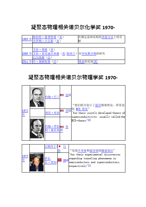
凝聚态物理相关诺贝尔化学奖1970-1985 年赫伯特·豪普特曼(美)杰罗姆·卡尔勒(美)在测定晶体结构的直接方法上的贡献2000 年艾伦·黑格(美)艾伦·麦克迪尔米德(美/新西兰)白川英树(日)对导电聚合物的研究2011 年丹·谢赫特曼(以)准晶的发现[5]凝聚态物理相关诺贝尔物理学奖1970-1972年约翰·巴丁美国“他们联合创立了超导微观理论,即常说的BCS 理论”"for their jointly developed theory ofsuperconductivity, usually called theBCS-theory"[73]利昂·库珀美国约翰·罗伯特·施里弗国美1973年江崎玲于奈日本“发现半导体和超导体的隧道效应”"for their experimental discoveriesregarding tunneling phenomena insemiconductors and superconductors,respectively"[74]伊瓦尔·贾埃弗挪威国英 “他理论上预测出通过隧道势垒的超电流的性质,特别是那些通常被称为约瑟夫森效应 布赖 的现象” 恩·戴"for his theoretical predictions of the 维·约瑟 properties of a supercurrent through a 夫森 tunnel barrier, in particular those phenomena which are generally known as the Josephson effect"[74]1977 年菲利普·沃伦·安德森国美“对磁性和无序体系电子结构的基础性理论研究”"for their fundamental theoretical investigations of the electronicstructure of magnetic and disorderedsystems"[78]内维尔·莫特 国英约翰·凡扶累克 国美年彼得·列昂尼多维奇·卡皮查苏联“低温物理领域的基本发明和发现” "for his basic inventions and discoveries in the area of low- temperature physics"[79]1982 年肯尼斯·威尔逊美国“对与相转变有关的临界现象理论的贡献”"for his theory for critical phenomena in connection with phase transitions"[83]1985 年克劳斯·冯·克利青德国“发现量子霍尔效应”"for the discovery of thequantized Hall effect"[86]特·鲁斯卡德国“电子光学的基础工作和设计了第一台显微镜"for his fundamental work in electron optics,electron microscope"格尔德·宾宁德国“研制"for their design of the scanningtunneling microscope"海因里希·罗雷尔瑞士约翰内斯·贝德诺尔茨德国“在发现"for their important break-through the discovery of superconductivity ceramic materials"卡尔·米勒瑞士皮埃尔吉勒纳法国“发现研究简单系统中有序现象的方法可以被推广到比较复杂的物质形式,特别是推广到"forfor studying order phenomena in simple systems can be generalized to morecomplexliquid crystals and polymers"1996年戴维·李美国“发现了在氦-3 里的超流动性”"for their discovery ofsuperfluidity inhelium-3"[97]道格拉斯·奥谢罗夫美国罗伯特·理查森美国2000年若雷斯·阿尔费罗夫俄罗斯“发展了用于高速电子学和光电子学的半导体异质结构”"for developing semiconductorheterostructures used in high-speed-and optoelectronics"[101]赫伯特·克勒默德国杰克·基尔比美国“在发明集成电路中所做的贡献”"for his part in the invention of theintegrated circuit"[101]2001年埃里克·康奈尔国美“在碱性原子稀薄气体的玻色-爱因斯坦凝聚态方面取得的成就,以及凝聚态物质属性质的早期基础性研究”"for the achievement of Bose-Einsteincondensation in dilute gases of alkaliatoms, and for early fundamental studiesof the properties of the condensates"[102]卡尔·威曼国美沃尔夫冈·克特勒国德2003年阿列克谢·阿布里科索夫美国俄罗斯“对超导体和超流体理论做出的先驱性贡献”"for pioneering contributions tothe theory of superconductors andsuperfluids"[104]维塔利·金俄罗斯兹堡安东尼·莱格特英国美国2007 年艾尔伯·费尔法国“发现巨磁阻效应”"for the discovery of giant magnetoresistance"[108]彼得·格林贝格德国2009 年高锟英国 美国 [110] “在光学通信领域光在纤维中传输方面的突破性成就” "for groundbreaking achievementsconcerning the transmission of light infibers for optical communication"[111]威拉 德·博伊尔 美国“发明半导体成像器件电荷耦合器件” "for the invention of an imaging semiconductor circuit – the CCD sensor"[111]乔治·史密斯美国2010 年安德烈·海姆荷兰俄罗斯“在二维石墨烯材料的开创性实验”"for groundbreaking experimentsregarding the two-dimensionalmaterial graphene"[112]康斯坦丁·诺沃肖洛夫英国俄罗斯。
2-1 Thermodynamics
ThermodynamicsThermodynamicsThermodynamics is a branch of physics which deals with the energy and work of a system Thermodynamics is the study of the effect of work, heat, and energy on the system.Power (W) = Rate at which energy is being transferred Work (J) ‐ amount of energy transferred from one system to another2ThermodynamicsThere are three principal laws of thermodynamics. Each law leads to the definition of thermodynamic properties which help us to understand and predict the operation of a physical system - Zeroth Law - First Law; Work, Heat, and Energy - Second Law; Entropy3The The Zero(th) Zero(th) Law LawThis law states that if object A is in thermal equilibrium with object B, and object B is in thermal equilibrium with object C, then object C is also in thermal equilibrium with object A. This law allows us to build thermometers.“C” for methane at +15C = 2.2 kJ/kg KThe concept of thermodynamic equilibrium, in which two objects have the same temperature. If we bring two objects that are initially at different temperatures into physical contact, they eventually achieve thermal equilibrium. During the process of reaching thermal equilibrium, heat is transferred between the objects. The amount of heat transferred delta Q is proportional to the temperature difference delta T 5 between the objects and the heat capacity c of the object.The amount of heat transferred delta Q is proportional to the temperature difference delta T between the objects and the heat capacity c of the object.6First First Law Law of of Thermodynamics ThermodynamicsThe first law introduces the concept that heat and work are equivalent. It states that: The heat lost from a source is equal to the total heat gained and work done on bodies that receive that heat.Second Second Law Law of of Thermodynamics ThermodynamicsThe second law introduce the concept of directional heat flow. It states that: Heat always flows from the hot body to a cooler one.Heat Heat Engine EngineForward Heat EngineA forward heat engine has a positive work output such as Rankine or Brayton cycle. Applying the first law of thermodynamics to the cycle gives: Q1 - Q2 - W = 0 The second law of thermodynamics states that the thermal efficiency of the cycle η has an upper limit (the thermal efficiency of the Carnot cycle), i.e. It can be shown that: Q1 > W, which means that it is impossible to convert the whole heat input to work and Q2 > 0, which means that a minimum of heat supply to the cold reservoir is necessary.Heat Heat Engine EngineForward Heat EngineHeat engine is defined as a device that converts heat energy into mechanical energy or more exactly a system which operates continuously and only heat and work may pass across its boundaries. The operation of a heat engine can best be represented by a thermodynamic cycle.Heat Heat Engine EngineReverse Heat EngineA reverse heat engine has a positive work input such as heat pump and refrigerator. Applying the first law of thermodynamics to the cycle gives: - Q1 + Q2 + W = 0 In case of a reverse heat engine the second law of thermodynamics is as follows: It is impossible to transfer heat from a cooler body to a hotter body without any work input i.e. W>0 which means that the co-efficiency of performance for a heat pump is greater than unity.Heat Heat Engine EngineReverse Heat EngineThe effectiveness of a reversed heat engine is defined in terms of a coefficient of performance (COP). The COP for a refrigerator is defined as: COP2 = Q2 / W and for a heat pump as: COP1 = Q1 / WEnthalpy Enthalpy Enthalpy is a thermodynamic measure of the total heat content of a liquid or vapor at a given temperature and is expressed in energy per unit mass (k Joules per 1 kg) from absolute zero. Therefore, for a liquid/vapor mixture, it will be seen that it is the sum of the enthalpy of the liquid plus the latent heat of vaporizationhx = h′+ χ(h″- h″) χ: Dryness factorEnthalpy Enthalpy -- Pressure Pressure In the previous examples the transition temperatures of water were 0° C and 100° C at atmospheric pressure. By altering pressure, we will affect the transitional temperature. When the relationship of enthalpy to pressure is plotted on a chart the resulting diagram is known as Mollier diagram.Enthalpy EnthalpyFrom a study of the FIRST LAW of thermodynamics, we find that the internal energy of a gas is also a state variable. - For a gas, a useful additional state variable is the enthalpy which is defined to be the sum of the internal energy E plus the product of the pressure p and volume V. Using the symbol H for the enthalpy: H=E+p*V - Propulsion engineers use the specific enthalpy in engine analysis more than the enthalpy itself. For a system with heat transfer Q and work W, the change in internal energy E from state 1 to state 2 is equal to the difference in the heat transfer into the system and the work done by the system: E2 - E1 = Q - W15Enthalpy Enthalpy- For the special case of a constant pressure process, the work done by the gas is given as the constant pressure p times the change in volume V: W = p * [V2 - V1] - Substituting into the first equation, we have: E2 - E1 = Q - p * [V2 - V1] - Let's group the conditions at state 2 and the conditions at state 1 together: (E2 + p * V2) - (E1 + p * V1) = Q - The (E + p * V) can be replaced by the enthalpy H; H2 - H1 = Q16Enthalpy EnthalpyFrom our definition of the heat transfer, we can represent Q by some heat capacity coefficient Cp times the temperature T. (H2 - H1) = Cp * (T2 - T1) -The SPECIFIC HEAT CAPACITY cp is called the specific heat at constant pressure and is related to the universal gas constant of the equation of state. This final equation is used to determine values of specific enthalpy for a given temperature. - Enthalpy is used in the energy equation for a fluid. Across shock waves, the total enthalpy of the gas remains a constant.17Entropy Entropy- Entropy, like temperature and pressure, can be explained on both a macro scale and a micro scale. Since thermodynamics deals only with the macro scale, the change in entropy delta S is defined here to be the heat transfer delta Q into the system divided by the temperature T: delta S = delta Q / T, dS = dQ / T - For gases, there are two possible ways to evaluate the change in entropy. We begin by using the first law of thermodynamics: dE = dQ - dW - If we use the definition of the enthalpy H of a gas: H = E + p * V, Then, dH = dE + p dV + V dp18Entropy Entropy- Substitute into the first law equation: dQ = dH - V dp - p dV + p dV - dQ = dH - V dp is an alternate way to present the first law of thermodynamics. For an ideal gas, the equation of state is written: p * V = R * T ; R is the gas constant - The heat transfer of a gas is equal to the heat capacity times the change in temperature; in differential form: dQ = C * dT - If we have a constant volume process, the formulation of the first law gives: dE = dQ = C (constant volume) * dT19Entropy Entropy- If we assume that the heat capacity is constant with temperature, we can use these two equations to define the change in enthalpy and internal energy. If we substitute the value for p from the equation of state, and the definition of dE in the first energy equation, we obtain: dQ = C (constant volume) * dT + R * T dV / V - Similarly substituting the value of V from the equation of state, and the definition of dH we obtain the alternate form: dQ = C (constant pressure) * dT - R * T dp / p - Substituting these forms for dQ into the differential form of the entropy equation gives: dS = C (constant volume) * dT / T + R * dV / V, and dS = C (constant pressure) * dT / T - R * dp / p20Entropy Entropy- These equations can be integrated from condition "1" to condition "2" to give: S2 - S1 = Cv * ln ( T2 / T1) + R * ln ( V2 / V1), and S2 - S1 = Cp * ln ( T2 / T1) - R * ln ( p2 / p1) - If we have a constant volume process, the second term in the equation is equal to zero, since v2/v1 = 1. We can then determine the value of the specific heat for the constant volume process. But if we have a process that changes volume, the second term in the equation is not zero. We can think of the first term of the equation as the contribution for a constant volume process, and the second term as the additional change produced by the change in volume. A similar type of argument can be made for the equation used for a change in pressure.21Operation Operation of of a a Simple Simple Cargo Cargo Reliq Reliq System System• There are two main types of liquefaction plants, namely: • Direct Reliquefaction Cycle; and Indirect Reliquefaction Cycle.In a Direct Reliquefaction Cycle, the evaporated or displaced cargo vapour is compressed, condensed and returned to the tank. This is the most commonly used system.••In an Indirect Reliquefaction Cycle, an external refrigeration system is employed to condense the cargo vapour without it being compressed. This cycle requires a very cold refrigerant and large surfaces. Enthalpy is a thermodynamic measure of the total heat content of a liquid or vapour at a given temperature and is expressed in energy per unit mass (k Joules per 1 kg) from absolute zero. Therefore, for a liquid/vapour mixture, it will be seen that it is the sum of the enthalpy of the liquid plus the latent heat of vaporisation.22Operation Operation of of a a Simple Simple Cargo Cargo System SystemVapour from cargo tankbCondensera dCompressorSeawaterTankcExpansion ValveReceiverHeatWith an understanding of the gas laws and the law of thermodynamics, the operation of the simple cargo system on board a liquefied gas ship can be followed. The cargo tank contains cold liquid, although it is insulated, some heat will still come through from outside. This is a consequence of second law of thermodynamics. This heat will overcome the latent heat of vaporisation and so some of the cargo will boil off. The vapour formed will raise the pressure in the tank. The vapour is drawn off and passed to a compressor.Operation Operation of of a a Simple Simple Cargo Cargo System SystemVapour from cargo tankbCondensera dCompressorSeawaterTankcExpansion ValveReceiverHeatThe work done by the compressor raises the temperature of the vapour according to the first law of thermodynamics. This temperature rise necessary so that it becomes hotter than the cooling medium that is subsequently used to cool it again.Operation Operation of of a a Simple Simple Cargo Cargo System SystemVapour from cargo tankbCondensera dCompressorSeawaterTankcExpansion ValveReceiverHeatThe hot gas or vapour now passes to a condenser where it is cooled by seawater. The removal of heat means that the molecules slow down and the vapour condenses to form a warm liquid. This liquid is also under pressure. The liquid is then passed through an expansion valve that reduces the pressure. This results in a partial evaporation, which causes the temperature of the bulk liquid to fall back down to tank temperature.Operation Operation of of a a Simple Simple Cargo Cargo System SystemVapour from cargo tankbCondensera dCompressorSeawaterTankcExpansion ValveReceiverHeatSo cold condensate is returned to the tank. These valves are also referred as JouleThompson valves, the physicist who discovered the cooling-expansion phenomenon. It is important to note that the joule-Thompson expansion results in cooling because the small amount of gas generated absorbs its latent heat of vaporisation from some of liquid.Operation Operation of of a a Simple Simple Cargo Cargo System SystemVapour from cargo tankbCondensera dCompressorSeawaterTankcExpansion ValveReceiverHeatJoule-Thompson expansion takes place at constant Enthalpy. The real cooling effect of this cycle is the removal of sensible heat and the latent heat of vaporisation from the full flow of gas as it condensed and cooled.28Operation Operation of of a a Simple Simple Cargo Cargo Reliq Reliq System SystemPressurecb aEnthalpyd29Ammonia Reliq Proces – direct single stage+33C 11.7 bar+140C 11.7 barCondenserExpansion valve Cargo Tank-33C 1.031 barCompressor-33C 1.031 bar3031Mollier Mollier Chart Chart of of Methane MethaneThe thermodynamic calculation of various gases or the liquids is done by using the thermodynamic diagram in general. Five (5) values of:1.pressure p, 2.specific volume v, 3.temperature T, 4.heat content h or i (enthalpy) 5.entropy sare used for the thermodynamic calculation. The p - i diagram is a so-called Mollier diagram, and “pressure p” is shown on VERICAL Axis and the “heat content h” (enthalpy i) on horizontal axisEnthalpyMollier Mollier Chart Chart of of Methane MethaneIsoEnthalpyMollier Mollier Chart Chart of of Methane MethaneThe following characteristics are included in this diagram:connected.)① Iso-bar(It is the horizontal in the line where the point of the same pressure was② Iso-enthalpy line (The normal in the line where the point of same was connected. )liquid and the right side are moist steam at the left of this line. )③ Saturated liquid line (In the line where the saturated liquid is shown, the under cooling ④ Saturated vapor line (In the line where the saturated vapor is shown, moist steamthe right side are superheated steam at the left of this line. ) andnormal in the liquid, and the line of a right descending in moist steam in the horizon and superheated steam as well as the isobar. )⑤ Iso-thermal (In the line where the same point of the temperature is shown, near the⑥ Iso-entropy curve (Line where point of the same entropy was connected) ⑦ Iso-specific volume line (Line where point of the same bulkiness was connected) ⑧ Iso-Dryness line (Line where point of constant dryness was connected. Dryness X = 0.1,it means that 10% dry saturated steam in moist steam.) 34Mollier Mollier Chart Chart of of Methane MethaneK Kj/K j/KgK gKCR I TI CA LC Con onst stan ant tT Tem empe pera ratu ture re oC oCTEConstant Constant Enthalpy Enthalpy kcal/kg kcal/kg or or Kj/kg Kj/kgC Con onst stan ant tE Ent ntro ropy pyGAS AREAM PE RA TURE=-82 .5C)CRITICAL PRESSURE (ie. CH4 = 43 Bar)IsoSUB COOLED LIQUIDS SA AT TU UR RA AT TE ED DV VA AP PO OU UR RL LI IN NE EL LII Q QU UII D DS SA AT TU UR RA AT TE ED Di spec o s IS CON e olum fi c VL LII N NE Ekg m3/ E M OLU V T TANSUPERHEATED VAPOURArea of PV=mRTSATURATED REGION – LIQUID / VAPOR MIXTURELATENT HEAT OF VAPORISATIONEnthalpyPRACTICAL USE OF MOLLIER DIAGRAM361ST EXAMPLE DIFFERENCE IN VOLUME BETWEEN LNG LIQUID AND LNG VAPOR AT SAME TEMPERATURE37Specific Volume 0.00235 m3/kgFor Density 425 kg/m3 (1/425 = 0.00235)s e ime m lu 55 t o V 2 ic ce f i ec ren p S iffe D.66 ity 1 s n e For Dfic V i c e Sp3/kg m 0 .600 0 e olum 001/ 1 m3 ( 0.6 .66 = kg/LNG Liquid >>> LNG Vapour at Boiling temp – 160 C1.4 51. LNG liquid2. LNG Vapour38Specific Volume 0.00235 m3/kgFor Density 425 kg/m3 (1/425 = 0.00235)Specific Volume change from LNG Liquid – 160 C >>> LNG Vapour at 20 C = Difference 619 timesSpecific Volume 1.45000 m3/kg @ 20CFor Density 0.69 kg/m3 (1/0.696 = 1.45 m3/kg1.4 51. LNG Liquid 3. LNG Vapour @ 20C 39LATENT HEAT REQUIRED FROM LIQUID to VAPOR KJ / KGLNG liquidLNG VapourLNG Latent Heat = 675 – 164 kj/kg = 511 kj/kgEnthalpy 164 kj/kg Enthalpy 675 kj/kg 40SENSITIVE HEAT KJ / kg C (K)Sensitive Heat from – 160 C to – 100 = 800 kj/kg ‐ 675 kj/kg = 125 kj/kg For 1 kg temperature to increase 60 C required 125 kj i.e. 125 kj / 60 C = Cp = 2.083 kJ/kg/CLNG VapourLNG VapourEnthalpy 675 kj/kgEnthalpy 800 kj/kg 41Mollier Mollier Chart ChartIn summary, it can be seen that the heat flowing into the tank has been returned to the environment via the seawater, together with the additional work done by Mollier chart. Point ‘a’ represents the vapour in the dome of the tank. As it passes to the compressor it picks up some heat. The compressor raises the temperature and pressure of the gas to point ‘b’ it is then cooled and condensed and becomes a saturated liquid at point ‘c’ in the condenser. The expansion valve then produces cold liquid with a proportion of vapour and this is returned to the tank at point ‘d’.Pressurecb aEnthalpyd。
BCS-BEC渡越过程中超冷费米原子气体的相干特性与非线性效应研究

BCS-BEC渡越过程中超冷费米原子气体的相干特性与非线性效应研究【摘要】:玻色-爱因斯坦凝聚(Bose-Einsteincondensation,BEC)是指当温度低于某一临界值时玻色子体系中大量粒子凝聚到一个或几个量子态的现象。
BEC是量子统计物理学的基本结论之一,是超流与超导现象的物理根源。
尽管费米子不能直接发生BEC,但通过Cooper配对等机制可形成费米子对。
这些费米子对如同(准)复合玻色子,从而可以发生BEC,导致费米体系的超导和超流。
近年来理论与实验研究表明,当粒子间的相互作用从吸引变为排斥时,费米子体系可以实现从Bardeen-Cooper-Schrieffer(BCS)超流到BEC的转变。
事实上,BCS与BEC只不过是BCS-BEC渡越(BCS-BECcrossover)过程的两个极限而已。
由于激光冷却与囚禁技术的发展与成功应用,科学家们已能使稀薄原子气体的温度降低到纳开的数量级,从而实现弱相互作用玻色原子(如87Rb,23Na等)气体的BEC及费米原子(6Li,40K等)气体的超低温冷却与量子简并,并进而通过Feshbach共振技术实现费米原子气体的超流以及从BCS态到BEC的渡越(BCS-BECcrossover)。
这些重大进展使得超冷原子物理成为原子分子物理、非线性与量子光学、统计和凝聚态物理等学科十分活跃的交叉前沿研究领域。
目前超冷费米气体已成为国际物理学界的研究热点之一。
无论是从基础物理研究的角度(包括物质波光学、量子调控、高温超导体等强关联体系的量子模拟、夸克-胶子等离子体和中子星的研究等),还是从发展精密光谱与精密测量等高新技术应用方面(包括研制原子激光、原子干涉仪、原子芯片、原子钟与光钟等)这些研究都有十分重要的意义。
超流费米原子气体理论研究的一个重要方法是使用量子多体理论。
由于问题的复杂性,既使对于简化了的哈密顿量,适用于整个BCS-BEC渡越的微观理论至今还未能建立起来。
英语文献

Thermodynamics (from the Greek θερμη, therme, meaning "heat" and δυναμις, dynamis, meaning "power") is a branch of physics that studies the effects of changes in temperature, pressure, and volume on physical systems at the macroscopic scale by analyzing the collective motion of their particles using statistics.[1]In this context, heat means "energy in transit" and dynamics relates to "movement;" thus, thermodynamics is the study of the movement of energy and how energy instills movement. Historically, thermodynamics developed out of need to increase the efficiency of early steam engines.[2]Typical thermodynamic system—heat moves from hot (boiler) to cold (condenser), (both not shown) and work is extracted, in this case by a series of pistons.The starting point for most thermodynamic considerations are the laws of thermodynamics, which postulate that energy can be exchanged between physical systems as heat or work.[3]The first law of thermodynamics states a universal principle that processes or changes in the real world involve energy, and within a closed system the total amount of that energy does not change, only its form (such as from heat of combustion to mechanical work in an engine) may change. The second law gives a direction to that change by specifying that in any change in any closed system in the real world the degree of order of the system's matter and energy becomes less, or conversely stated, the amount of disorder (entropy) of the system increases.[4]In thermodynamics, interactions between large ensembles of objects are studied and categorized. Central to this are the concepts of system and surroundings. A system comprises particles whose average motions define the system's properties, which are related to one another through equations of state defining the relations between state variables such as temperature, pressure, volume, and entropy. State variables can becombined to express internal energy and thermodynamic potentials, which are useful for determining conditions for equilibrium and spontaneous processes.[5]With these tools, thermodynamics describes how systems respond to changes in their surroundings. This can be applied to a wide variety of topics in science and engineering, such as engines, phase transitions, chemical reactions, transport phenomena, and even black holes. The results of thermodynamics are essential for other fields of physics and for chemistry, chemical engineering, aerospace engineering, mechanical engineering, cell biology, biomedical engineering, and materials science to name a few.[6]Thermodynamics, with its insights into the relations between heat, energy, and work as exemplified in mechanical systems, provides a foundation for trying to understand the behavior and properties of biological, social, and economic systems, which generally maintain an ordered pattern only by consuming a sustained flow of energy.Thermodynamics is the branch of physical science concerned with heat and its relation to other forms of energy and work. It defines macroscopic variables (such as temperature, entropy, and pressure) that describe average properties of material bodies and radiation, and explains how they are related and by what laws they change with time. Thermodynamics does not describe the microscopic constituents of matter, and its laws can be derived from statistical mechanics.Thermodynamics can be applied to a wide variety of topics in science and engineering, such as engines, phase transitions, chemical reactions, transport phenomena, and even black holes. The results of thermodynamics are essential for other fields of physics and for chemistry, chemical engineering, aerospace engineering, mechanical engineering, cell biology, biomedical engineering, materials science, and are useful for other fields such as economics.[1][2]Thermodynamics is one of the best logically structured branches of physics and has become one of the classical branches of theoretical physics.[citation needed]Much of the empirical content of thermodynamics is contained in its four laws. The first law specifies that energy can be exchanged between physical systems as heat and thermodynamic work.[3]The second law concerns a quantity called entropy, that expresses limitations, arising from what is known as irreversibility, on the amount of thermodynamic work that can be delivered to an external system by a thermodynamic process.[4]Historically, thermodynamics developed out of a desire to increase the efficiency of early steam engines, particularly through the work of French physicist Nicolas Léonard Sadi Carnot (1824) who believed that the efficiency of heat engines was the key that could help France win the Napoleonic Wars.[5] Scottish physicist Lord Kelvin was the first to formulate a concise definition of thermodynamics in 1854:[6]Thermo-dynamics is the subject of the relation of heat to forces acting between contiguous parts of bodies, and the relation of heat to electrical agency.Initially, the thermodynamics of heat engines concerned mainly the thermal properties of their 'working materials', such as steam. This concern was then linked to the study of energy transfers in chemical processes, for example to the investigation, published in 1840, of the heats of chemical reactions[7] by Germain Hess, which was not originally explicitly concerned with the relation between energy exchanges by heat and work. Chemical thermodynamics studies the role of entropy in chemical reactions.[8][9][10][11][12][13][14][15][16] Also, statistical thermodynamics, or statistical mechanics, gave explanations of macroscopic thermodynamics by statistical predictions of the collective motion of particles based on the mechanics of their microscopic behavior.The plain term 'thermodynamics' refers to macroscopic description of bodies and processes.[17]"Any reference to atomic constitution is foreign to ... thermodynamics".[18] The qualified term 'statistical thermodynamics' refers to descriptions of bodies and processes in terms of the atomic constitution of matter.Thermodynamics is built on the study of energy transfers that can be strictly resolved into two distinct components, heat and work, specified by macroscopic variables.[19][20]Thermodynamic equilibrium is one of the most important concepts for thermodynamics. As the systems and processes of interest are taken further from thermodynamic equilibrium, their thermodynamical study becomes a little more involved but also of much more practical value. In many important cases, such as heat engines or refrigerators, the systems consist of many subsystems at different temperatures and pressures. Thermodynamics is a practical science and also deals with these inhomogeneous dynamic systems provided the thermodynamical parameters are well-defined. The present article takes a gradual approach to the subject, starting with a focus on cyclic processes and thermodynamic equilibrium, and then gradually beginning to further considernon-equilibrium systems.For thermodynamics and statistical thermodynamics to apply to a process in a body, it is necessary that the atomic mechanisms of the process fall into just two classes: those so rapid that, in the time frame of the process of interest, the atomic states effectively visit all of their accessible range, and those so slow that their effects can be neglected in the time frame of the process of interest.[21] The rapid atomic mechanisms mediate the macroscopic changes that are of interest for thermodynamics and statistical thermodynamics, because they quickly bring the system near enough to thermodynamic equilibrium. "When intermediate rates are present, thermodynamics and statistical mechanics cannot be applied."[21] The intermediate rate atomic processes do not bring the system near enough to thermodynamic equilibrium in the time frame of the macroscopic process of interest. This separation of time scales of atomic processes is a theme that recurs throughout the subject.Basic for thermodynamics are the concepts of system and surroundings.[12][22]There are two fundamental kinds of entity in thermodynamics, states of a system, and processes of a system. This allows two fundamental approaches to thermodynamic reasoning, that in terms of states of a system, and that in terms of cyclic processes of a system.For thermodynamics and statistical thermodynamics to apply to a process in a body, it is necessary that the atomic mechanisms of the process fall into just two classes: those so rapid that, in the time frame of the process of interest, the atomic states effectively visit all of their accessible range, and those so slow that their effects can be neglected in the time frame of the process of interest.[21] The rapid atomic mechanisms mediate the macroscopic changes that are of interest for thermodynamics and statistical thermodynamics, because they quickly bring the system near enough to thermodynamic equilibrium. "When intermediate rates are present, thermodynamics and statistical mechanics cannot be applied."[21] The intermediate rate atomic processes do not bring the system near enough to thermodynamic equilibrium in the time frame of the macroscopic process of interest. This separation of time scales of atomic processes is a theme that recurs throughout the subject.Basic for thermodynamics are the concepts of system and surroundings.[12][22]There are two fundamental kinds of entity in thermodynamics, states of a system, and processes of a system. This allows two fundamental approaches to thermodynamic reasoning, that in terms of states of a system, and that in terms of cyclic processes of a system.A thermodynamic system can be defined in terms of its states. In this way, a thermodynamic system is a macroscopic physical object, explicitly specified in terms of macroscopic physical and chemical variables which describe its macroscopic properties. The macroscopic state variables of thermodynamics have been recognized in the course of empirical work in physics and chemistry.[13]A thermodynamic system can also be defined in terms of the processes which it can undergo. Of particular interest are cyclic processes. This was the way of the founders of thermodynamics in the first three quarters of the nineteenth century.The surroundings of a thermodynamic system are other thermodynamic systems that can interact with it. An example of a thermodynamic surrounding is a heat bath, which is considered to be held at a prescribed temperature, regardless of the interactions it might have with the system.The macroscopic variables of a thermodynamic system in thermodynamic equilibrium, in which temperature is well defined, can be related to one another through equations of state or characteristic equations.[23][24][25][26] They express the constitutive peculiarities of the material of the system.Classical thermodynamics is characterized by its study of materials that have equations of state that express relations between mechanical variables and temperature that are reached much more rapidly than any changes in the surroundings. A classical material can usually be described by a function that makes pressure dependent on volume and temperature, the resulting pressure being established much more rapidly than any imposed change of volume or temperature.[27]This is another expression of the concept of separation of time scales of atomic processes mentioned above.Thermodynamic facts can often be explained by viewing macroscopic objects as assemblies of very many microscopic or atomic objects that obey Hamiltonian dynamics.[12][28][29] The microscopic or atomic objects exist in species, the objects of each species being all alike. Because of this likeness, statistical methods can be used to account for the macroscopic properties of the thermodynamic system in terms of the properties of the microscopic species. Such explanation is called statistical thermodynamics; also often it is also referred to by the term 'statistical mechanics', though this term can have a wider meaning, referring to 'microscopic objects', such as economic quantities, that do not obey Hamiltonian dynamics.[28]The study of thermodynamical systems has developed into several related branches, each using a different fundamental model as a theoretical or experimental basis, or applying the principles to varying types of systems.[edit] Classical thermodynamicsClassical thermodynamics is the description of the states (especially equilibrium states) and processes of thermodynamical systems, using macroscopic, empirical properties directly measurable in the laboratory. It is used to model exchanges of energy, work, heat, and matter, based on the laws of thermodynamics. The qualifier classical reflects the fact that it represents the descriptive level in terms of macroscopic empirical parameters that can be measured in the laboratory, that was the first level of understanding in the 19th century. A microscopic interpretation of these concepts was provided by the development of statistical thermodynamics.[edit] Statistical thermodynamicsStatistical thermodynamics, also called statistical mechanics, emerged with the development of atomic and molecular theories in the second half of the 19th century and early 20th century, supplementing thermodynamics with an interpretation of the microscopic interactions between individual particles or quantum-mechanical states. This field relates the microscopic properties of individual atoms and molecules to the macroscopic, bulk properties of materials that can be observed on the human scale, thereby explaining thermodynamics as a natural result of statistics, classical mechanics, and quantum theory at the microscopic level.[edit] Chemical thermodynamicsChemical thermodynamics is the study of the interrelation of energy with chemical reactions and chemical transport and with physical changes of state within the confines of the laws of thermodynamics.[edit] Thermodynamic equilibriumEquilibrium thermodynamics studies transformations of matter and energy in systems at or near thermodynamic equilibrium. In thermodynamicequilibrium, a system's properties are, by definition, unchanging in time. In thermodynamic equilibrium no macroscopic change is occurring or can be triggered; within the system, every microscopic process is balanced by its opposite; this is called the principle of detailed balance. A central aim in equilibrium thermodynamics is: given a system in awell-defined initial state, subject to specified constraints, to calculate what the equilibrium state of the system will be.[40]Within a simple isolated thermodynamic system in thermodynamic equilibrium, in the absence of externally imposed force fields, all properties of the material of the system are spatially homogeneous.[41]Much of the basic theory of thermodynamics is concerned with homogeneous systems in thermodynamic equilibrium.[8][42]Most systems found in nature or considered in engineering are not in thermodynamic equilibrium, exactly considered. They are changing or can be triggered to change over time, and are continuously and discontinuously subject to flux of matter and energy to and from other systems.[43] For example, according to Callen, "in absolute thermodynamic equilibrium all radioactive materials would have decayed completely and nuclear reactions would have transmuted all nuclei to the most stable isotopes. Such processes, which would take cosmic times to complete, generally can be ignored.".[43] Such processes being ignored, many systems in nature are close enough to thermodynamic equilibrium that for many purposes their behaviour can be well approximated by equilibrium calculations.[edit] Quasi-static transfers between simple systems are nearly in thermodynamic equilibrium and are reversibleIt very much eases and simplifies theoretical thermodynamical studies to imagine transfers of energy and matter between two simple systems that proceed so slowly that at all times each simple system considered separately is near enough to thermodynamic equilibrium. Such processes are sometimes called quasi-static and are near enough to being reversible.[44][45][edit] Natural processes are partly explained by tendency towards thermodynamic equilibrium and are irreversibleSimple isolated thermodynamic systems, as time passes, tend naturally towards thermodynamic equilibrium. In the absence of externally imposed force fields, they become homogeneous in all their local properties.Many thermodynamic processes can be can be modeled by compound or composite systems, consisting of several or many contiguous component simple systems, initially not in thermodynamic equilibrium, but allowed to transfer mass and energy between them. Natural thermodynamic processes can be explained in terms of a tendency towards thermodynamic equilibrium within simple systems and in transfers between contiguous simple systems. Such natural processes are irreversible.[46][edit] Non-equilibrium thermodynamicsNon-equilibrium thermodynamics[47]is a branch of thermodynamics that deals with systems that are not in thermodynamic equilibrium; it is also called thermodynamics of irreversible processes. Non-equilibrium thermodynamics is concerned with transport processes and with the rates of chemical reactions.[48] Non-equilibrium systems can be in stationary states that are not homogeneous even when there is no externally imposed field of force; in this case, the description of the internal state of the system requires a field theory.[49][50][51] One of the methods of dealing with non-equilibrium systems is to introduce so-called 'internal variables'. These are quantities that express the local state of the system, besides the usual local thermodynamic variables; in a sense such variables might be seen as expressing the 'memory' of the materials. Hysteresis may sometimes be described in this way. In contrast to the usual thermodynamic variables, 'internal variables' cannot be controlled by external manipulations.[52]This approach is usually unnecessary for gases and liquids, but may be useful for solids.[53] Many natural systems still today remain beyond the scope of currently known macroscopic thermodynamic methods.[edit] System modelsA diagram of a generic thermodynamic systemAn important concept in thermodynamics is the thermodynamic system, a precisely defined region of the universe under study. Everything in the universe except the system is known as the surroundings. A system is separated from the remainder of the universe by a boundary which may benotional or not, but which by convention delimits a finite volume. Exchanges of work, heat, or matter between the system and the surroundings take place across this boundary.The boundary is simply a surface around the volume of interest. Anything that passes across the boundary that effects a change in the internal energy needs to be accounted for in the energy balance equation. The volume can be the region surrounding a single atom resonating energy, as Max Planck defined in 1900; it can be a body of steam or air in a steam engine, such as Sadi Carnot defined in 1824; it can be the body of a tropical cyclone, such as Kerry Emanuel theorized in 1986 in the field of atmospheric thermodynamics; it could also be just one nuclide (i.e. a system of quarks) as hypothesized in quantum thermodynamics.Boundaries are of four types: fixed, moveable, real, and imaginary. For example, in an engine, a fixed boundary means the piston is locked at its position; as such, a constant volume process occurs. In that same engine, a moveable boundary allows the piston to move in and out. For closed systems, boundaries are real while for open system boundaries are often imaginary.Generally, thermodynamics distinguishes three classes of systems, defined in terms of what is allowed to cross their boundaries.Interactions of thermodynamic systemsType of system Mass flow Work HeatOpenClosedIsolatedIn theoretical studies, it is often convenient to consider the simplest kind of thermodynamic system. This is defined variously by different authors.[77][78][56][79][80][81] For the present article, the following definition will be convenient, as abstracted from the definitions of various authors.A region of material with all intensive properties continuous in space and time is called a phase. A simple system is for the present article defined as one that consists of a single phase of material with no interior partitions.Engineering and natural processes are often described as compounds of many different component simple systems, sometimes with unchanging or changing partitions between them.[edit] States and processesThere are two fundamental kinds of entity in thermodynamics, states of a system, and processes of a system. This allows two fundamental approaches to thermodynamic reasoning, that in terms of states of a system, and that in terms of cyclic processes of a system.The approach through states of a system requires a full account of the state of the system as well as a notion of process from one state to another of a system, but may require only a partial account of the state of the surroundings of the system or of other systems.The notion of a cyclic process does not require a full account of the state of the system, but does require a full account of how the process occasions transfers of matter and energy between the system and its surroundings, which must include at least two heat reservoirs at different temperatures, one hotter than the other. In this approach, the notion of a properly numerical scale of temperature is a presupposition of thermodynamics, not a notion constructed by or derived from it.The method of description in terms of states has limitations. For example, processes in a region of turbulent flow, or in a burning gas mixture, or in a Knudsen gas may be beyond "the province of thermodynamics".[82][83][84] This problem can sometimes be circumvented through the method of description in terms of cyclic processes. This is part of the reason why the founders of thermodynamics often preferred the cyclic process description.[edit] Thermodynamic state variablesWhen a system is at thermodynamic equilibrium under a given set of conditions of its surroundings, it is said to be in a definite thermodynamic state, which is fully described by its state variables.If a system is simple as defined above, and is in thermodynamic equilibrium, and is not subject to an externally imposed force field, such as gravity, electricity, or magnetism, then it is homogeneous, that is say, spatially uniform in all respects.[85]In a sense, a homogeneous system can be regarded as spatiallyzero-dimensional, because it has no spatial variation.If a system in thermodynamic equilibrium is homogeneous, then its state can be described by a few physical variables, which are mostly classifiable as intensive variables and extensive variables.[51][86][87][12][28]Examples of extensive thermodynamic variables are total mass and total volume. Examples of intensive thermodynamic variables are temperature, pressure, and chemical concentration; intensive thermodynamic variables are defined at each spatial point and each instant of time in a system. Physical macroscopic variables can be mechanical or thermal.[28] Temperature is a thermal variable; according to Guggenheim, "the most important conception in thermodynamics is temperature."[12]Intensive variables are defined by the property that if any number of systems, each in its own separate homogeneous thermodynamic equilibrium state, all with the same respective values of all of their intensive variables, regardless of the values of their extensive variables, are laid contiguously with no partition between them, so as to form a new system, then the values of the intensive variables of the new system are the same as those of the separate constituent systems. Such a composite system is in a homogeneous thermodynamic equilibrium. Examples of intensive variables are temperature, chemical concentration, pressure, density of mass, density of internal energy, and, when it can be properly defined, density of entropy.[88]Extensive variables are defined by the property that if any number of systems, regardless of their possible separate thermodynamic equilibrium or non-equilibrium states or intensive variables, are laid side by side with no partition between them so as to form a new system, then the values of the extensive variables of the new system are the sums of the values of the respective extensive variables of the individual separate constituent systems. Obviously, there is no reason to expect such a composite system to be in in a homogeneous thermodynamic equilibrium. Examples of extensive variables are mass, volume, and internal energy. They depend on the total quantity of mass in the system.[89]Though, when it can be properly defined, density of entropy is an intensive variable, for inhomogeneous systems, entropy itself does not fit into this classification of state variables.[90][91] The reason is that entropy is a property of a system as a whole, and not necessarily related simply to its constituents separately. It is true that for any number of systems each in its own separate homogeneous thermodynamic equilibrium, all with the same values of intensive variables, removal of the partitions between the separate systems results in a composite homogeneous system in thermodynamic equilibrium, with all the values of its intensive variables the same as those of the constituent systems, and it is reservedly orconditionally true that the entropy of such a restrictively defined composite system is the sum of the entropies of the constituent systems. But if the constituent systems do not satisfy these restrictive conditions, the entropy of a composite system cannot be expected to be the sum of the entropies of the constituent systems, because the entropy is a property of the composite system as a whole. Therefore, though under these restrictive reservations, entropy satisfies some requirements for extensivity defined just above, entropy in general does not fit the above definition of an extensive variable.Being neither an intensive variable nor an extensive variable according to the above definition, entropy is thus a stand-out variable, because it is a state variable of a system as a whole.[90]A non-equilibrium system can have a very inhomogeneous dynamical structure. This is one reason for distinguishing the study of equilibrium thermodynamics from the study of non-equilibrium thermodynamics.The physical reason for the existence of extensive variables is the time-invariance of volume in a given inertial reference frame, and the strictly local conservation of mass, momentum, angular momentum, and energy. As noted by Gibbs, entropy is unlike energy and mass, because it is not locally conserved.[90] The stand-out quantity entropy is never conserved in real physical processes; all real physical processes are irreversible.[92] The motion of planets seems reversible on a short time scale (millions of years), but their motion, according to Newton's laws, is mathematically an example of deterministic chaos. Eventually a planet will suffer an unpredictable collision with an object from its surroundings, outer space in this case, and consequently its future course will be radically unpredictable. Theoretically this can be expressed by saying that every natural process dissipates some information from the predictable part of its activity into the unpredictable part. The predictable part is expressed in the generalized mechanical variables, and the unpredictable part in heat.There are other state variables which can be regarded as conditionally 'extensive' subject to reservation as above, but not extensive as defined above. Examples are the Gibbs free energy, the Helmholtz free energy, and the enthalpy. Consequently, just because for some systems under particular conditions of their surroundings such state variables are conditionally conjugate to intensive variables, such conjugacy does not make such state variables extensive as defined above. This is another reason for distinguishing the study of equilibrium thermodynamics from the study of non-equilibrium thermodynamics. In another way of thinking, this explains why heat is to be regarded as a quantity that refers to a process and not to a state of a system.。
均匀碱性费米气中BCS-BEC混合系统动力学

V0 . 6 No 3 12 .
Sp 20 e .0 8
ห้องสมุดไป่ตู้
—
均 匀 碱 性 费 米 气 中 B S—B C混 合 系统 动 力学 C E
孙玲姣
( 湖北 民族 学 院 信 息工 程 学院 , 北 恩 施 4 50 ) 湖 4 00
摘要 : 研究 了均 匀碱性 费米 气的 B S—B C混合 区域 的动力 学行为 , C E 讨论 了在温度 T K时。 =O 通过分别 改变平 衡 时分子 分解 阈能 2。和“ v 泵浦” 参量 时混合 系统 的混沌动力 学. 关键 词: 费米气 ; 色 一爱因斯坦凝聚( E ) 序参量 玻 BC ;
Absr t tac :W e i v sia e t e d n mi s o i r Femi n e a k l g s s i n e tg t h y a c funf m r o i l a i a e n BCS — BEC r s o e . W e o cos v r
束缚分子之间相互耦合 ’( l 图 描述 了它们 的相互作用过程 ) 同时也考 虑了分子与分子之间 的相互 作 , 用 , 动量层 分 布如 图 2所 示 , 以采用 玻 色 一费米 模型 的 哈密 顿量 来 描述有 N个 原子 的巨正则 系综 : 所
H=∑ ( 一 )
l to rd s u so o T=OK , n x l i y s o e c a t y a c yv r ig t e t r s o d e e g f i u ic si n t mi a d e p i t h w t h oi d n misb a yn h e h l n r y o cl h c h i l ul r f a q i b i m t ts2 0a d “ u ” p r mee ,e p c v l . n e i u s e v n a p mp a a t rS r s e t e y i
- 1、下载文档前请自行甄别文档内容的完整性,平台不提供额外的编辑、内容补充、找答案等附加服务。
- 2、"仅部分预览"的文档,不可在线预览部分如存在完整性等问题,可反馈申请退款(可完整预览的文档不适用该条件!)。
- 3、如文档侵犯您的权益,请联系客服反馈,我们会尽快为您处理(人工客服工作时间:9:00-18:30)。
a r X i v :c o n d -m a t /0608282v 3 [c o n d -m a t .s t a t -m e c h ] 22 F eb 2007Thermodynamics of the BCS-BEC crossoverR.Haussmann,1W.Rantner,2S.Cerrito,3,2and W.Zwerger 31Fachbereich Physik,Universit¨a t Konstanz,D-78457Konstanz,Germany2Institut f¨u r Theoretische Physik,Universit¨a t Innsbruck,Technikerstrasse 25,A-6020Innsbruck,Austria3Technische Universit¨a t M¨u nchen,James-Franck-Strasse,D-85748Garching,Germany(Dated:published version,8February 2007)We present a self-consistent theory for the thermodynamics of the BCS-BEC crossover in the normal and superfluid phase which is both conserving and gapless.It is based on the variational many-body formalism developed by Luttinger and Ward and by DeDominicis and Martin.Trun-cating the exact functional for the entropy to that obtained within a ladder approximation,the resulting self-consistent integral equations for the normal and anomalous Green functions are solved numerically for arbitrary coupling.The critical temperature,the equation of state and the entropy are determined as a function of the dimensionless parameter 1/k F a ,which controls the crossover from the BCS-regime of extended pairs to the BEC-regime of tightly bound molecules.The tightly bound pairs turn out to be described by a Popov-type approximation for a dilute,repulsive Bose gas.Even though our approximation does not capture the critical behaviour near the continuous superfluid transition,our results provide a consistent picture for the complete crossover thermody-namics which compare well with recent numerical and field-theoretic approaches at the unitarity point.PACS numbers:03.75.Ss,03.75.Hh,74.20.FgI.INTRODUCTIONThe problem of a two component attractive Fermi gas near a resonance of the s-wave scattering length describ-ing the effective interaction is one of the basic many-body problems which has been brought into focus by the re-cent realization of molecular condensates in ultra-cold Fermi gases [1,2,3]and the subsequent exploration of the crossover from a Bose-Einstein-Condensate (BEC)to a BCS-like state of weakly bound fermion pairs [4].Clear signatures for the existence of paired fermion su-perfluidity with cold atoms have been provided by spec-troscopic measurements of the gap [5]and the observa-tion of a vortex lattice on the BCS-side of the transition [6].The ability of tuning the interaction in cold Fermi gases through Feshbach resonances relies on the resonant coupling of the scattering state near zero energy of two colliding atoms with a bound state in a closed channel [7].A particularly challenging problem arises right at the Feshbach resonance,where the two-particle scatter-ing length is infinite [8,9].Precisely at this point and for broad Feshbach resonances,where the range r ⋆of the effective interaction is much smaller than the mean in-terparticle spacing [10,11,12,13],the full many-body problem has the Fermi energy εF as the only energy scale.As pointed out by Ho [14],the thermodynamics of the unitary Fermi gas is then a function only of the dimensionless temperature θ=T/T F .More generally,as emphasized recently by Nikolic and Sachdev [15],the universality also extends to the behaviour away from the Feshbach resonance,as long as the broad resonance con-dition k F r ⋆≪1is obeyed.Thus,for instance,the criti-cal temperature T c /T F for the transition to superfluidity is a universal function of the inverse coupling constant 1/k F a .A quantitative theoretical understanding of the many-body problem near a Feshbach resonance has been devel-oped recently through numerical calculations.In partic-ular,at zero temperature and for a homogeneous system,fixed-node Green function Monte Carlo calculations pro-vide quantitative results for the gap parameter [16],the equation of state [17],and also the momentum distribu-tion,the condensate fraction and the pair size [18]of the ground-state for arbitrary values of 1/k F a .As expected in the case of an s-wave resonance [19],these quanti-ties all evolve continously as the coupling is varied from the BCS to the BEC-limit.An important ingredient in these results is their account for the repulsive interaction between strongly bound dimers in the BEC-limit with scattering length a dd ≈0.60a >0[20].This interac-tion is missing in the early qualitative descriptions of the T =0BCS-BEC crossover problem by Eagles [21]and Leggett [22],which are based on using the standard BCS-groundstate as a variational Ansatz for arbitrary coupling [23].Beyond a purely numerical approach,the BCS-BEC crossover problem has recently become amenable also to analytical methods via an ǫ=4−d expansion [24].It is based on the observation [25]that at the uni-tarity point in d =4(i.e.the point where a two-particle bound state appears)the two-component Fermi gas is in fact an ideal Bose gas,because a zero range interaction in d =4can bind a state only at infinitely strong at-traction.In two dimensions,in turn,binding appears at arbitrary small couplings and the unitary Fermi gas in d ≤2coincides with a non-interacting one [25].Within a field theoretic description,the physically interesting 3D problem can thus be approached by extrapolating ex-pansions from the upper and lower critical dimensions d =4and d =2respectively [26].At finite temper-ature,numerical calculations are available for the ther-2modynamics at the unitarity point.They are based on an auxiliaryfield quantum Monte-Carlo method for the continuum problem[27]and on a diagrammatic determi-nant Monte-Carlo method for the negative U-Hubbard model[28].Field-theoretic results atfinite temperature, which open the possibility for controlled and systematic expansions for the crossover thermodynamics have been obtained very recently by Nishida[26]within an expan-sion around both the upper or lower critical dimension and by Nikolic and Sachdev[15]within a1/N expansion for a2N component Fermi gas.Our aim in the following is to present a self-consistent many-body theory for the thermodynamics of resonantly interacting fermions at arbitrary temperatures and de-tuning,which directly addresses the physically relevant case of a three dimensional,two-component Fermi gas. The theory is based on a conserving,so-calledΦ-derivable approach to the many-body problem,in which the exact one-or two-particle Green functions serve as an infinite set of variational parameters.It is an extension of earlier work by one of us[29,30,31]and employs a combina-tion of the Luttinger-Ward and DeDominicis-Martin ap-proach for obtaining the grand canonical potential and the entropy,respectively.The condition of gaplessness is enforced by a modified coupling constant,thus account-ing for the proper low energy behaviour in terms of a Bogoliubov-Anderson mode.We provide quantitative re-sults for the critical temperature,the equation of state and the entropy near the Feshbach-resonance as a func-tion of both T/T F and1/k F a.In spite of the fact that the critical behaviour at the continuous superfluid transition is not captured correctly in our approach,which gives rise to a weakfirst order transition,the results provide a quantitative and consistent picture of the crossover which obeys thermodynamic relations at the percent level.Our variational method is complementary both to purely nu-merical and tofield theoretic approaches to the problem. The results can be used e.g.to predict thefinal tempera-ture reached after an adiabatic ramp across the Feshbach-resonance starting deeply in the BEC-regime[32]or to determine the size of the atom cloud in a harmonic trap near unitarity as a function of temperature.The paper is organized as follows:in Sec.II we in-troduce our model and the basic many-body formalism necessary for deriving a set of self-consistent equations for the Green and vertex functions which are the variational parameters of the theory.The complete thermodynam-ics is then determined by integrals of the momentum and frequency dependent Green functions.It is shown that with a modified coupling constant,the theory can be for-mulated in a way consistent with Ward identities,which guarantees a gapless Bogoliubov-Anderson mode for arbi-trary strength of the coupling.In Sec.III we discuss the numerical solution,providing quantitative results for the critical temperature,the pressure,internal energy and the entropy of the BCS-BEC crossover both in the nor-mal and superfluid phase.They are compared both with experimental and theoretical results based on numerical andfield-theoretic approaches.Finally in Sec.IV we give a brief summary,and indicate open problems.II.A MANY-BODY THEORY OF RESONANTLY INTERACTING FERMIONSIn order to describe interacting fermions near a Fesh-bach resonance,it is in general necessary to include the resonant,closed channel bound state explicitely,e.g. within a Bose-Fermi-resonance model[33,34].As has been shown for instance by Diener and Ho[11],how-ever,the situation can be simplified in the case of broad Feshbach resonances,where the effective range r⋆of the resonant interaction is much smaller than both the back-ground scattering length a bg and the Fermi wavelength λF.In this limit,which is in fact appropriate for the existing experimental studies of the BCS-BEC crossover problem in6Li[5]and in40K[1],the problem can be reduced to a single channel Hamiltonian with an instan-taneous interaction[10,11,12,13].The associated effec-tive two-body interaction is thus described by a pseudo-potential V(r)∼δ(r)(appropriately renormalized,see below)with a strength proportional to the scattering lengtha=a bg 1−∆B2m[∇ψ+σ(r)][∇ψσ(r)]+1g=1(2π)dmthe bare interaction parameter g0must be taken to zero in the limit where the cutoffdiverges.The associatedlimiting process g0→−0accounts for the replacement of the bare potential(2.3)by a pseudopotential with theproper scattering length.While the formulas are derived for arbitrary space dimensions d,eventually we consider fermions for d=3.In this case the scattering amplitude g is simply connected to the s-wave scattering length a given in(2.1)by g=4π 2a/m.In the following,we consider a homogeneous situationdescribed by a grand canonical distribution atfixed tem-perature and chemical potential.The thermodynamic properties thus follow from the grand partition functionZ=Tr{exp(−β[ˆH−µˆN])}(2.5) and the associated grand potentialΩ=Ω(T,µ)=−β−1ln Z(2.6) which is directly related to the pressure p viaΩ=−pV. Within our simplified model,where the range of the in-teraction is set to zero,the Fermi system is described by three parameters:the temperature T,the chemical potentialµand the s-wave scattering length a.Apart from an overall scale,the thermodynamics thus depends only on two dimensionless ratios.It is convenient to re-place the chemical potentialµby the fermion density n=k3F/3π2,which defines the Fermi wave number k F and the Fermi energyεF= 2k2F/2m as characteristic length and energy scales.The equilibrium state is then uniquely determined by only two parameters:the dimen-sionless temperatureθ=T/εF(we choose units for the temperature in which k B=1),and the dimensionless in-teraction strength v=1/k F a.In the special case B=B0 of an infinite scattering length(the so-called unitarity limit),the parameter v drops out and the resulting ther-modynamic quantities are universal functions ofθ[14].A.Luttinger-Ward formalismThe BCS-BEC crossover is controlled by two physical phenomena.Thefirst one is connected with the forma-tion of pairs due to the attractive interaction.The sec-ond one is the transition to superfluidity below a certain critical temperature T c.In the BCS-limit,the formation of pairs and the superfluid transition are simultaneous. The transition is driven by the thermal breakup of pairs, i.e.by excitations which may be described by a purely fermionic theory.With increasing strength of the inter-action,however,there is an increasingly wide range of temperatures where bound pairs coexist with unpaired fermions.In the BEC-limit,pair formation,as a chem-ical equilibrium between bound and dissociated atoms, occurs at a temperature scale much higher than the su-perfluid transition.The latter is driven by collective ex-citations of a then purely bosonic system.A proper de-scription of the crossover thus requires to account for both bosonic and fermionic excitations simultaneously.Following the formalism developed by Luttinger and Ward[35]for non-superfluid interacting Fermi systems, the grand thermodynamic potential(2.6)can be ex-pressed as a unique functional of the Green functionGσσ′(r−r′,τ−τ′)= δσσ′G(r−r′,τ−τ′)εσσ′F(r−r′,τ−τ′)−εσσ′F∗(r′−r,τ−τ′)−δσσ′G(r′−r,τ′−τ)(2.7) in the formΩ[G]=β−1 −1−1321ll −1l321lΦ[G ]=+FIG.1:The functional Φ[G ]in self-consistent ladder approx-imation.The propagator lines are dressed lines identified by the matrix Green function G .the fermion system is a Bose liquid of dilute atom pairs.In this limit the ladder approximation describes the for-mation of pairs (two-particle problem)exactly,however the interaction between the pairs (four-particle problem)only approximately [20,37].In particular the resulting dimer-dimer scattering length is given by the Born ap-proximation a (B )dd =2a .B.DeDominicis-Martin formalismAn extension of the Luttinger-Ward formalism was given by DeDominicis and Martin [38].They introduce up to four external fields,which couple to products of one,two,three,and four field operators,and perform the Legendre transformations to the corresponding con-jugate variables -the Green functions.For fermion sys-tems only two external fields are relevant which couple to even products of fermion field operators.The related two conjugate variables of the Legendre transformation are the one-particle Green function G and the two-particle Green function G 2.Within our approach below,the second Legendre transformation is performed explicitely.A more convenient conjugate variable is then the ver-tex function Γwhich is related to G 2by (2.15)below.Thus,DeDominicis and Martin obtain a thermodynamic potential which is a functional of both G and Γ.More precisely,it turns out that the relevant functional is the entropy S =F (2)where F (2)[G,Γ]=12Tr {ln[1−12¯Γ+12¯Γ]2−(1/4!)[¯Γ]2}+K (2)[G,Γ](2.10)(see (61)in the second paper of Ref.38and identify G 1=G ,C 2=−Γ,and ¯C2=−¯Γtherein).¯Γis defined in (2.14)below.The formalism of DeDominicis and Martin is ideally adapted to describe the BCS-BEC crossover because it explicitly deals with the one-particle Green function G ,which represent the properties of the single fermions,and the vertex function Γ,which describes the eventu-ally purely bosonic properties of the fermion pairs (both condensed or noncondensed).In particular,a full imple-mentation of their formalism is needed to correctly ac-count for four particle correlation,which is necessary to obtain the exact result a dd =0.60a for the dimer-dimer scattering length in the BEC limit.As in standard thermodynamics,the entropy (2.10)is maximized under the constraints that all conserved quantities are kept constant.For the interacting fermion system defined by the Hamiltonian (2.2)the conservedquantities are the internal energy U = ˆHand the par-ticle number N =−1diagrams,where the propagator lines and the vertices are dressed and identified by the one-particle Green function G and by the vertex functionΓ,respectively.In order to understand the physical meaning of the various contributions to the thermodynamic potential, we note that the Luttinger-Ward formalism and the DeDominicis-Martin formalism are related to each other by a Legendre transformation,in which the bare two-particle interaction as an externalfield is transformed into the two-particle Green function G2.This Legendre transformation may be interpreted as a renormalization procedure.Since the two-particle Green function G2is expressed in terms of the vertex functionΓbyG2,X1X2X3X4=G X1X3G X2X4−G X1X4G X2X3−G X1X2G X3X4−G X1Y1G X2Y2ΓY1Y2Y3Y4G Y3X3G Y4X4,(2.15)the bare two-particle interaction is replaced by the vertex functionΓas the renormalized interaction,which is the many-particle generalization of the scattering amplitude g.We may compare the functionals(2.8)and(2.10)di-rectly with each other.Thefirst trace in(2.10)is iden-tified by the trace in(2.8),which describe the contribu-tion of single particles to the grand canonical potential and entropy,respectively.The second trace and the func-tional K(2)[G,Γ]in(2.10)which represent the interaction terms are related to the functionalΦ[G]in(2.8).By close inspection(see(62)in Ref.38)wefind that the second trace in(2.10)represents the inverted perturbation series of ladder diagrams.It includes both particle-particle and particle-hole ladders,which describe the scattering and formation of pairs and it also includes bubble diagrams, which describe the screening of the interaction.These three types of diagrams and mixtures of them arise because the vertices are symmetrized so that each of them can be expressed as a sum of three unsymmetrized vertices.As a result,the self-consistent ladder approx-imation of the functionalΦ[G]shown in Fig.1can be reformulated within the formalism of DeDominicis and Martin in the following way:the second trace is ap-proximated by keeping only the particle-particle ladders and the complicated functional K(2)[G,Γ]is set equal to zero.This neglects the screening of the interaction due to particle-hole excitations(see Subsec.III A below) and also the coupling between collective excitations and bound pairs.In the following subsections we employ the formal-ism of DeDominicis and Martin to construct explicit ex-pressions for S[G,Γ],U[G,Γ],and N[G].From(2.12) we obtain the functionalΩ[G,Γ].The stationarity cri-teria(2.13)imply two self-consistent equations for the Green function G and the vertex functionΓ.Solv-ing the second equation with respect toΓand insert-ing the resulting vertex function intoΩ[G,Γ]we recover the functionalΩ[G]of the Luttinger-Ward formalism to-gether with the stationarity condition(2.9).This fact explicitely demonstrates the equivalence of the Luttinger-Ward and DeDominics-Martin formalism for our approx-imation scheme(see(2.41)-(2.43)below)once the appro-priate stationarity conditions have been taken into ac-count.C.Thermodynamic potentialsThe formalism of Luttinger and Ward[35]allows to calculate directly the grand thermodynamic potentialΩ.The functionalΦ[G]has been evaluated explicitly in Ref.31.Inserting this result into(2.8)we obtainΩ[G]=−L d d d kβ ωn Tr −ln[G(k,ωn)]+[G0(k,ωn)−1G(k,ωn)−1]+L d g0|F(0,0)|2+1(2π)d1(2π)d1quencies are denoted by small letters,while the bosonic wave vectors and Matsubara frequencies are denoted by capitalletters.Inthesecondtermof (2.16)the anoma-lous Green function is identified by F (0,0)=F (r =0,τ=0).The formulas are derived for an arbitrary di-mension of space d .The volume is assumed to be a cube with edge length L and periodic boundary conditions,where the limit L →∞is taken.The strength of the attractive interaction is included by the bare interaction parameter g 0.The kinetic energy of the atoms εk = 2k 2/2m and the chemical potential µare implicitly included via the free matrix Green func-tion G 0(k ,ωn ),which is related to the free normal Green functionG 0(k ,ωn )=1/[−i ωn +εk −µ](2.19)and the free anomalous Green functionF 0(k ,ωn )=0(2.20)by a formula which is analogous to (2.17).The tem-perature T is included explicitly by the factors 1/βand implicitly by the Matsubara frequencies ωn and Ωn .As evident from (2.16),the formalism of Luttinger and Ward,though including the exact single-particle Green function,still contains the bare coupling constant g 0.In the DeDominicis-Martin formalism the bare coupling is renormalized and replaced by the exact vertex function Γvia a second Legendre transformation.The correspond-ing functional S [G,Γ]=F 2[G,Γ],is just the dimension-less entropy as given in ((2.10))As discussed above we restrict the second trace in (2.10)to the particle-particle ladders and by the nature of our interaction potential (2.3)to s-wave scattering.Furthermore,we omit the 2-line irreducible Feynman dia-grams by setting K (2)[G,Γ]=0.This approximation cov-ers the essential features of the crossover problem namely the formation of pairs and their condensation.Within our ladder approximation,the DeDominicis-Martin for-malism thus leads to an expression for the entropy of the formS [G,Γ]=βL dd d kβωnTr −ln[G (k ,ωn )]+[−i ωn G (k ,ωn )−1]+1(2π)d12in front of ¯Γdisap-pears.Furthermore,the quadratic terms in the second trace cancel.Another important quantity to consider is the internal energy U .With the help of the delta potential (2.3)we find for the expectation value of the Hamiltonian (2.2),U =d dr σ22d drσσ′g 0 ψ+σ(r )ψ+σ′(r )ψσ′(r )ψσ(r ) .(2.23)The second term contains an average of four fermion field operators which can be expressed in terms of the two-particle Green function G 2.Following the formalism of DeDominicis and Martin [38]and using (2.15)the two-particle Green function can be expressed by four terms.The first three terms represent the three possibilities to factorize the two-particle Green function into products of two one-particle Green functions according to the Wick theorem.These terms provide the Hartree energy,the Fock energy,and the Bogoliubov energy.The fourth term is the connected part of the two-particle Green function and provides the correlation energy.Taking all terms together we obtain the internal energyU[G,Γ]=−2L d d d kL d d d Kβ Ωn g0Tr χ(K,Ωn)−χ(K,Ωn)Γ(K,Ωn)χ(K,Ωn) .(2.24)2Finally,the particle number N is defined by the aver-ageN= ˆN = d d r σ ψ+σ(r)ψσ(r) (2.25)which can be expressed in terms of the normal Greenfunction in the standard formN[G]=−2L d d d kδΦ[G]βL dis represented by the nondiagonal elements of the matrixΣ1= 0∆∆∗0 .(2.32)In the second term of(2.30)Γis the matrix vertex func-tion,which is related to the matrix pair propagatorχbyΓ−1αα′(K,Ωn)=g−10δαα′+χαα′(K,Ωn).(2.33) Eventually,χis represented in terms of the matrix Green function by(2.18).Eq.(2.33)is just the Bethe-Salpeter equation in ladder approximation.It is responsible for the fact that the binding of fermion pairs is described appropriately.Taken together,we have now a set of self-consistent equations for the matrix Green function G and the matrix vertex functionΓwhich have to be solved numerically.Alternatively we can derive the self-consistent equa-tions by inserting the functional(2.12)of the formalism of DeDominicis and Martin into the related stationarity conditions(2.13).We obtain the Dyson equation(2.28) from thefirst condition and the Bethe-Salpeter equa-tion(2.33)from the second condition.In this way we prove that both the Luttinger-Ward formalism and the DeDominicis-Martin formalism are equivalent within our approximation.Unfortunately,in the present form,the matrix pair propagatorχdefined in(2.18)is divergent.While the sum over the Matsubara frequencies isfinite,the integral over the wave vector is ultraviolet divergent for dimen-sions d≥2.For this reason a renormalization is neces-sary.We define the regularized pair propagator byMαα′(K,Ωn)= d d kβ ωn Gαα′(K−k,Ωn−ωn)Gαα′(k,ωn)−m (2π)d1(2π)d F(k,τ=0)+∆mis the second term of the self energy(2.30).The otherself-consistent equations remain unchanged.The grandthermodynamic potential(2.16)is transformed intoΩ=−L d d d kβ ωn Tr −ln[G(k,ωn)]+[G1(k,ωn)−1G(k,ωn)−1]−L d|∆|22L d d d Kβ Ωn Tr −ln[Γ(K,Ωn)/g0] .(2.41) For a combination of the internal energy(2.24)and the particle number(2.26)we obtain the formulaU−µN=−L d d d kβ ωn Tr [G1(k,ωn)−1+i ωn]G(k,ωn)−L d|∆|22L d d d Kβ Ωn Tr [Γ(K,Ωn)/g0−1] .(2.42) The entropy(2.21)depends neither on G0nor on G1.We transform the formula intoS=βL d d d kβ ωn Tr −ln[G(k,ωn)]+[−i ωn G(k,ωn)−1]−1(2π)d1(2π)d 1g0,(2.45)while the mean-field formula for the combination of the internal energy and the particle number are U1−µN1=−L d d d kβ ωn Tr [G1(k,ωn)−1+i ωn]G1(k,ωn) −L d|∆|2(2π)d1In order to obtainfinite results,we must define the sums over the Matsubara frequencies as described in Appendix A.The sums can be evaluated explicitly.This yieldsΩ1=E0−1(2π)d ln[1+exp(−β(E k−µ)],(2.48)U1−µN1=E0+2L d d d k(2π)d (1−n k)ln(1−n k)+n k ln n k ,(2.50) which are the well known results of a BCS variational Ansatz for arbitrary coupling whereE0=−2L d d d k2 (E k−µ)−(εk−µ) −L d|∆|21(2π)dL d d d Kβ Ωn Tr −ln[Γ(K,Ωn)/g0] ,(2.54)2the correction for the combination of the internal energy and the particle number∆U −µ∆N =−L dd d k β ωnTr [G 1(k ,ωn )−1+i ωn ][G (k ,ωn )−G 1(k ,ωn )]−1(2π)d1(2π)d 12βLdd dK βΩnTr −ln[Γ(K ,Ωn )/g 0]+[Γ(K ,Ωn )/g 0−1] .(2.56)In formulas (2.54)-(2.56)the sums over the fermionic Matsubara frequencies ωn converge so that the regularization of Appendix A is not needed.However,the sums over the bosonic Matsubara frequencies Ωn are not well defined and must be regularized.Thus,for a numerical evaluation the formulas (2.54)-(2.56)must be transformed further,which will be done in the next subsection.H.Renormalization of the thermodynamic potentialsSince the interaction has zero range,the interaction strength g 0must be renormalized and replaced by the scat-tering amplitude g according to (2.4).In a first step we renormalize the mean-field formulas of the thermodynamic potentials.In (2.48)-(2.50)the interaction strength g 0does not occur explicitly.The integrals are thus finite and no renormalization is needed for these formulas.However,the condensation energy (2.51)contains two infinite terms,a divergent integral and the last term with the infinite factor 1/g 0,which compensate each other.By renormalizing the interaction strength we obtainE 0=−2L dd d k 2 (E k −µ)−(εk −µ)−|∆|2g (2.57)where both the integral and the last term are now separately finite.Note that the wave vector integrals in (2.48)-(2.50)and in (2.57)are finite in any spatial dimension d with 2<d <4.In a second step we renormalize the correction formulas.In the correction of the grand thermodynamic potential (2.54)we decompose ln[Γ(K ,Ωn )/g 0]=ln[Γ(K ,Ωn )/g ]+ln[g/g 0].The separated term ln[g/g 0]can be neglected because it does not depend on the Matsubara frequencies Ωn .Following the arguments of Appendix A the Matsubara-frequency sum of this term is zero.Thus,for the correction of the grand thermodynamic potential we obtain the renormalized formula∆Ω=−L dd d k β ωnTr −ln[G 1(k ,ωn )−1G (k ,ωn )]+[G 1(k ,ωn )−1G (k ,ωn )−1]+1(2π)d1(2π)d1(2π)d1(2π)d1(2π)d 1interchange the orders of the integrals and sums,and combine Γwith one of the G into the self energy ˜Σby (2.40).Finally,wereplace ˜Σin favor of G and G 1by using the Dyson equation (2.39).The bosonic integral and sum are transformed into a fermionic integral and sum.Hence,the second term of (2.55)can be combined with the first term.As a result we finally obtain∆U −µ∆N =−1(2π)d12Ldd d kβωnTr G 1(k ,−ωn )−1[G (k ,ωn )−G 1(k ,ωn )](2.62)which is essential for a stable numerical evaluation of the correction term.The Matsubara-frequency sum is evaluated by using (A3).The wave-vector integral is finite.The correction of the entropy (2.56)is renormalized in an analogous way.Alternatively,we use the thermodynamic relation (2.44).As a result we obtain∆S =βL d d d kβ ωnTr −ln[G 1(k ,ωn )−1G (k ,ωn )]+[G 1(k ,ωn )−1G (k ,ωn )−1]−1(2π)d12βLdd d KβΩnTr −ln[Γ(K ,Ωn )/g ] .(2.63)The final results are the mean-field formulas (2.48)-(2.50)together with (2.57)and the correction formulas (2.58),(2.62),and (2.63).In these formulas each term by itself is finite.Eventually,the thermodynamic potentials are obtained by adding the terms together according to Ω=Ω1+∆Ω,S =S 1+∆S ,etc..I.Symmetry breaking and Thouless criterionThe interacting fermion system is invariant under the symmetry transformationψσ(r )→e iλψσ(r ),ψ+σ(r )→e −iλψ+σ(r )(2.64)which is related to a global change of phase of thefermion fields by λ.The superfluid phase breaks this symmetry since the order parameter ∆is transformed as ∆→e 2iλ∆.Clearly,however,the thermodynamic potentials must remain invariant under a global change of the phase both in the normal and in the superfluid state.In the superfluid,the free energy increase associ-ated with a slowly varying phase λ(r )vanishes like (∇λ)2.By Goldstone’s theorem,this implies the existence of modes whose energy vanishes in the long wave-lengthlimit.For a neutral superfluid,this is the well knownBogoliubov-Anderson mode.It has a sound like disper-sion ω(k )=ck and is physically related to fluctuations of the phase of the order parameter.In technical terms,the existence of zero-energy collec-tive modes can be derived from Ward identities related to the symmetry transformation.By considering the grand thermodynamic potential Ω[G ],in Ref.31the Ward iden-tityY Y ′Γ−1XX ′,Y ′Y δλΣY Y ′=0(2.65)has been derived (see (2.57)in Ref.31).Here δλΣXX ′is the variation of the self energy under the transforma-tion (2.64)with an infinitesimal phase change δλ.This quantity may be interpreted as the generalized order pa-rameter of the system.On the other hand,Γ−1XX ′,Y Y ′is the inverse vertex function.For a short-hand notation the indices X ,X ′and Y ,Y ′are used,which represent a combination X =(r ,τ,σ,α)of the space variable r ,the imaginary time τ,the spin index σ,and the Nambu index α.According to (2.65)the inverse vertex function Γ−1may be interpreted as a linear operator which acts on the order parameter δλΣ.In the superfluid state the order。