Growth from 1997-

合集下载

1997 - sowing the seeds, nurturing growth and harvesting the rewards

Marks will be awarded for content, organization, grammar and appropriacy. Failure to follow the above instructions may result in a loss of marks.
Moreover, whereas the growth of crops nurturing, the mastery of knowledge also requires reinforcement. A lazy farmer often neglects fertilizing the soil, only to find his crops in poor conditions and finally have a bad year. Similarly, a sluggish student also fails because he does not bother to consolidate what he acquires in class. In fact, learning does not happen once and for all. This has been proved by the experiences of those successful university students. They review their lessons constantly. They never hesitate to ask the teachers for solutions to their puzzles. They also do a lot of reading related to what they learn in class. Thus they have a better command of knowledge than those who do not take the trouble. As a consequence, the industrious students generally have a greater prospect of success.

熊彼特增长模型英文教程--香港浸会大学-工商管理学院课件

innovators!
• James M. Utterback:
If a company only focuses on current product rather
than improving the quality, it will be swept out of market!
• Peter Druke:
12/4/2020
熊彼特增长模型英文教程--香港浸会大学 -工商管理学院
Literature Review of Schumpeterian Model
• How economy grows in Schumpeterian growth theory?
12/4/2020
熊彼特增长模型英文教程--香港浸会大学 -工商管理学院
Literature Review of Schumpeterian Model
*Capital-based growth theory emphasizes on the idea that the accumulation of capital (material capital and human capital) is the most important power to push the advancement of technology and economy.
market.
12/4/2020
熊彼特增长模型英文教程--香港浸会大学 -工商管理学院
Literature Review of Schumpeterian Model
• Creative destruction is the motivation of the development of capitalism. Additionally, the Schumpeterian growth theory which we define here does not order the process of innovation to be a process of creative destruction. Under the vertical innovation framework, process of innovation is a process of creative destruction, so old goods will be replaced by new goods. Whereas, under horizontal innovation framework, both the old and new goods will exist in the market.

人类发展指数 (HDI) 的计算

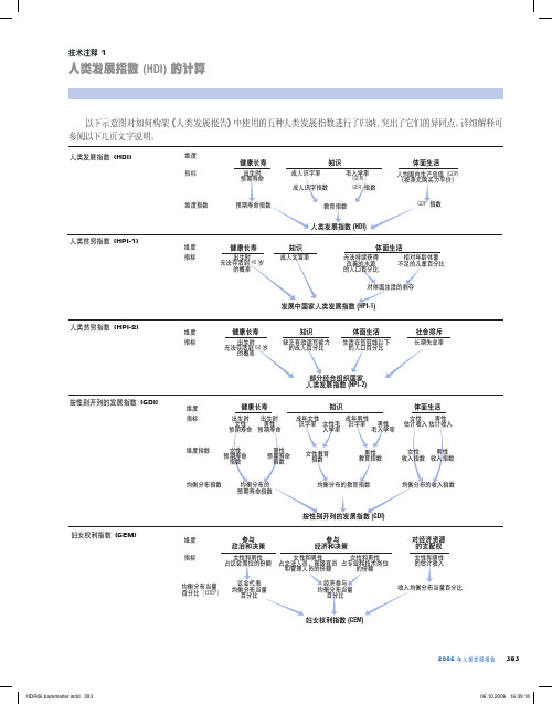
成人识字率 (%)
综合毛入学率 (%)
人均国内生产总值
（按美元购买力平价）
极大值极小值
85 25
100
0
100
0
40,000 100
计算 HDI 此 HDI 计算演示使用了巴西的数据。
1. 计算预期寿命指数预期寿命指数用于测度一个国家在出生时预期
寿命方面所取得的相对成就。就巴西来说，其 2004 年的预期寿命为 70.8 岁，所对应的预期寿命指数为 0.764。
40
.400
30
成人识字指数 = 88.6 – 0 = 0.886 100 – 0
毛入学指数 = 86 – 0 = 0.857 100 – 0
教育指数 = 2/3 （成人识字指数）+ 1/3 (毛入学指数)
20 10
0
成人识字率 (%)
毛入学率 (%)
.200 0 教育指数
= 2/3 (0.886) + 1/3 (0.857) = 0.876
预期寿命指数 = 70.8 – 25 = 0.764 85 – 25
2. 计算教育指数
90 阈值 85 岁
80 70.8
70
60
50
40
30 阈值 25 岁
20
0.764
预期寿命（岁）
1.00 .800 .600 .400 .200 0 预期寿命指数
教育指数衡量的是一个国家在成人识字及
初、中、高综合毛入学率两方面所取得的相对
GER 指数
教育指数
体面生活人均国内生产总值 (GDP)
（按美元购买力平价）
GDP 指数
人类贫穷指数 (HPI-1)
维度指标

Financial Deepening, Inequality, and Growth

Review of Economic Studies(2006)73,251–2930034-6527/06/00100251$02.00 c 2006International Monetary FundFinancial Deepening,Inequality,and Growth:A Model-BasedQuantitative Evaluation1ROBERT M.TOWNSENDUniversity of Chicago and Federal Reserve Bank of ChicagoandKENICHI UEDAInternational Monetary FundFirst version received August2001;ﬁnal version accepted April2005(Eds.)We propose a coherent uniﬁed approach to the study of the linkages among economic growth,ﬁnancial structure,and inequality,bringing together disparate theoretical and empirical literature.Thatis,we show how to conduct model-based quantitative research on transitional paths.With analytical andnumerical methods,we calibrate and make tractable a prototype canonical model and take it to an ap-plication,namely,Thailand1976–1996,an emerging market economy in a phase of economic expansionwith unevenﬁnancial deepening and increasing inequality.We look at the expected path generated bythe model and conduct robustness experiments.Because the actual path of the Thai economy is imag-ined here to be just one realization of many possible histories of the model economy,we construct acovariance-normalized squared error metric of closeness andﬁnd the best-ﬁt simulation.We also con-struct a conﬁdence region from a set of simulations and formally test the model.We broadly replicate theactual data and identify anomalies.1.INTRODUCTIONWe propose a coherent uniﬁed approach to the study of the linkages among economic growth,ﬁnancial structure,and inequality.Of course,the relationship betweenﬁnancial structure and economic growth has long been studied both empirically and theoretically.Yet,on the one hand, empirical studies have been mainly focused on statistical relationships without a serious study of underlying mechanisms that generate the observations.On the other hand,most theoretical studies have depicted clean but simple mechanisms without serious consideration given to the models’quantitative predictions.The same dichotomy between theory and empirical work exists in the literature on inequality and growth.Early seminal empirical contributions focusing on growth andﬁnancial structure are those of Goldsmith(1969),McKinnon(1973),and Shaw(1973).A more recent empirical treatment is by King and Levine(1993).This body of empirical work establishes thatﬁnancial deepening is at least an intrinsic part of the growth process and may be causal—that is,repressedﬁnan-cial systems harm economic growth.Theoretical efforts at modelling growth and endogenous ﬁnancial deepening include studies by Townsend(1978,1983)and Greenwood and Jovanovic (1990)(hereinafter referred to as GJ).Their models posit costly bilateral exchange or intermedi-ation costs—for example,aﬁxed cost to enter the formalﬁnancial system and marginal costs to1.The views expressed in this paper are those of the authors and do not necessarily represent those of the FRB Chicago,the Federal Reserve System,or the IMF.251252REVIEW OF ECONOMIC STUDIESsubsequent transactions.Other theoretical contributions such as those of Bencivenga and Smith (1991)turn intermediation on and off exogenously and have an external effect that makes growth with intermediation higher.Saint-Paul(1992)features limited diversiﬁcation and multiple equi-librium growth paths,some with developedﬁnancial systems and specialized technologies and others with the opposite.In turn,Acemoglu and Zilibotti(1997)show that capital accumulation is associated with increasing intermediation and that better diversiﬁcation,which comes with higher levels of wealth,reduces the variability of growth.Likewise well known are seminal contributions on growth and inequality.Kuznets(1955) posited that growth is associated with increasing and eventual decreasing inequality.Interest and controversies,especially with respect to cross-country regressions,have continued ever since.A recent paper,Forbes(2000),conﬁrms previous regression studies that high(initial)inequality is associated with low subsequent long-run growth butﬁnds that the relationship is the opposite for the medium term.Resting separately from this strand of the empirical literature are the deservedly well-known theoretical contributions more motivated by Kuznets’s original assertion that growth may bring increasing,and eventually decreasing,inequality—namely,Banerjee and Newman (1993),Aghion and Bolton(1997),Piketty(1997),and Lloyd-Ellis and Bernhardt(2000).We have a concern about this dichotomy between theories and empirical studies.Although most of the theoretical models characterize economic growth withﬁnancial deepening and chang-ing inequality as transitional phenomena,typical empirical research employs regression analysis toﬁnd a coefﬁcient capturing the effect ofﬁnancial depth or inequality on growth.The implicit assumptions of stationarity and linearity are incorrect,even after taking logs and lags,if the vari-ables of actual economies lie on complex transitional growth paths,as they do in the theoretical ing artiﬁcial data generated by a canonical model that by construction displays tran-sitional growth withﬁnancial deepening and increasing inequality,we can sometimes replicate the typical empirical results of the literature:ﬁnancial deepening appears to lead to subsequent higher growth,and inequality to subsequent lower growth.But the statistical signiﬁcance is weak and sensitive to initial history,timeframe,the inclusion of covariates,and so on.Evidently re-gression coefﬁcients are not informative about the underlying true relationships.In pointing this out,we add to the list of concerns which have been raised in recent literature—for example,in Banerjee and Duﬂo(2000).Taking a more constructive tack,we show how to conduct quantitative research on transi-tional growth paths—that is,how to test a model and learn something about actual economies from potential rejections.Our canonical model is based on GJ.2As a prerequisite for a numerical study,we need to characterize analytical properties as much as possible.GJ characterizes primar-ily the initial and asymptotic economy but leaves the all-important transitions somewhat unclear. GJ also studies only the log utility function and does not take its characterization of the log case to data.Here we extend the model to include a wider class of constant relative risk aversion (CRRA)utility functions.We characterize much of the transitional dynamics analytically and,in doing so,provide new results.The seemingly non-convex technology of participation is shown, under some conditions,to be convexiﬁed by the optimal choice of portfolio shares between risky and safe assets.Consequently,savings and portfolio choice are uniquely determined depending on the wealth level.In particular,ironically,those risk-averse households and businesses without access are not condemned to low-yield(though safe)technologies but rather shift towards risky2.There are a few other model-based contributions to empirical work on growth and wealth inequality.Álvarez and Díaz(2002)study evolution of wealth inequality in a nonstochastic neoclassical growth model with minimum con-sumption requirements and apply it to the U.S.economy.It is a calibration study of growth and inequality of wealth,but the growth rate is not affected by inequality of wealth because of perfect capital markets and identical incomes among households.Likewise De Nardi(2004)focuses on savings and bequests to explain wealth inequality in the U.S.and Sweden.De Nardi’s is a steady-state calibration exercise based on an overlapping generation model.This also contains an excellent review of the inter-generational inequality literature.TOWNSEND&UEDA A MODEL-BASED QUANTITATIVE EV ALUATION253 enterprises,especially as their wealth approaches a critical value.These make clear the rich and potentially complicated dynamics not obvious in the original GJ formulation.Indeed,the single valuedness of savings and portfolio choice facilitates further research into transitional dynamics using numerical methods and weﬁnd,for example,overall inequality movement is not neces-sarily monotonic on the growth path—it can increase,then decrease,and then increase again as it moves slowly towards its asymptotic steady state.Financial deepening and growth are not monotonic either.With the model made tractable,we take it to an application,namely,Thailand between1976 and1996,an emerging market economy that was in a phase of economic expansion with uneven ﬁnancial deepening and increasing(and then decreasing)inequality.The Thai economy serves as a prototypical example of the growth and inequality phenomena,pervasive in other countries, that motivate the growth,ﬁnancial deepening,and inequality ing the Thai Socio-Economic Survey(SES),Jeong(2000)ﬁnds that growth and inequality are strongly associated withﬁnancial deepening.We emphasize,however,that our methods are not peculiar to Thailand and we hope to extend the analysis to other countries.In the spirit of the business cycle literature,we calibrate the parameter values.Thus,the benchmark parameters are set from several sources.Data on the yields of relatively safe assets or occupations—5·4%per year for agriculture—and idiosyncratic shocks for business come from the Townsend-Thai data.3Risk aversion is set at values typically found in theﬁnancial economics literature,and the real rate of interest implied by a preference for current consumption is set at 4%.Aggregate shocks are difﬁcult to pin down,and we take advantage of the average and the variation of the observed real growth rate of the per capita gross domestic product(GDP)over the sample period.The marginal cost of utilizing theﬁnancial system is set at low values,but the higherﬁxed cost of entry is such that,as in the Thai SES,6%of the Thai population would have had access to theﬁnancial system in1976,using a distribution of wealth estimated from the same1976SES data.The model is simulated at these and nearby values to deliver predicted paths,which can be compared to the actual Thai data.Note that we are calibrating a non-steady-state stochastic model.The business cycle liter-ature calibrates around stochastic steady states,not transitions.For example,Krusell and Smith (1998)ﬁnd that a pseudo-representative agent model can almost perfectly characterize the be-haviour of the macroeconomic aggregates of an actual incomplete market economy with wealth heterogeneity among agents.This is not the case here.This different outcome stems from the fact that they look at business cycle implications in a stochastic steady state and also their model does not contain a source of non-linearity,such as theﬁxed cost to participate in theﬁnancial system in our model.There is also a literature on transitions or out-of-steady-state dynamics devoted to the study of depressions,but the models are deterministic(e.g.Hayashi and Prescott,2002). Indeed,it is a challenging task to calibrate transitional paths in a stochastic environment,because there is no precedent sensible statistic criteria for goodness ofﬁt.Here,we examine theﬁt of the model in three ways:the expected path,the best-ﬁt prediction,and the conﬁdence region.First,we look at the expected path of the model.It is broadly consistent with the actual pat-tern of growth with increasing inequality along withﬁnancial deepening.However,although the computed expected participation rate and the Theil index(an inequality measure)in the model almost trace out a smoothed version of the actual Thai data,the computed expected GDP growth rate is lower than the actual Thai path.We vary the key parameters and conduct robustness experiments,exploring some trade-offs.3.See Townsend,Paulson,Sakuntasathien,Lee and Binford(1997).254REVIEW OF ECONOMIC STUDIESSecond,we look at the best-ﬁt path among1000simulations.Because the actual path of the Thai economy is imagined here to be just one realization of many possible histories of the model economy,the actual Thai path should differ from the expected path of the model.We construct a metric of closeness between a simulated path and the actual data,considering the growth rate,ﬁnancial deepening,and inequality variables over the entire1976–1996period to be one particu-lar realization.We pick the best-ﬁt simulation under this metric.The best-ﬁt simulation shows a reasonable match with GDP growth rate,but misses a sharp upturn of theﬁnancial deepening in the mid-1980’s as well as the eventual downturn of inequality in the1990’s.Finally,we examine whether the actual Thai data lie within a conﬁdence region generated by the model,using covariance-normalized mean squared error criteria constructed solely from the model-generated histories.The model imposes sharp restrictions on the data,and indeed,at the benchmark parameter values,the model is rejected.But this guides us in identifying where the modelﬁts well and where it does not.Of course,we are not unaware of the tension in this paper between the working out of the details of a structural and well-articulated but highly abstract version of reality,on the one hand, and its serious application to data on the other hand.But the goal here is to show that these two pieces can be brought together.This,we believe,is the way to make progress towards under-standing the true relationships among endogenousﬁnancial deepening,economic development, and changing inequality.2.MODEL2.1.NotationThe model is a simple,tractable growth model with aﬁnancial sector.It is assumed that a large number of people live in the economy and they are consumers and entrepreneurs at the same time.More speciﬁcally,there is a continuum of agents in the economy as if with names indexed on the interval[0,1].At the beginning of each period,they start with their assets k t.After they consume c t,some portion of the assets,they use the remaining assets(i.e.savings s t)to engage in productive activities.An individual can engage in two types of productive activities:a safe but low-return occupa-tion and a high-risk,high-return business.The safe projects are assumed to returnδand the risky businesses are assumed to returnθt+ t,whereθt∈ is a shock common to all the people and t∈E is an idiosyncratic shock,different among people.An individual does not have to stick tothe same projects over time and she/he can choose portionφt∈[0,1]of her/his savings to invest in high-risk,high-return projects.Aﬁnancial institution provides two services to its customers in this simple model.First, aﬁnancial institution offers insurance for idiosyncratic shocks by pooling funds.Second,a ﬁnancial institution selects projects when people apply for loans by inferring the true aggre-gate shocks,and tell them if they should stay in the relatively safe occupation or engage in the high-risk,high-return business.44.An alternative interpretation is that the household puts money on deposit but then borrows toﬁnance a project under advice from the bank.Average repayment is determined by eitherθt orδ.But if risky projects are undertaken, low t households repay less,as if receiving insurance,and high t households repay more,as if paying premia,so as to repayθt on average.That is,the debt repayment is allowed to vary with idiosyncratic shocks.Either way,we recognize that this speciﬁcation of theﬁnancial sector’s advantages may be extreme.One could imagine less-than-perfect risk sharing,constrained by default or private information considerations,for example.One could also imagine less-than-perfect information about forthcoming realizations,as the number of bank clients engaged in any given activity(or sector/region)may be limited and,in any event,past experience in a given activity is only a limited guide to future shocks. However,this speciﬁcation ofﬁnancial services does make the model tractable.TOWNSEND &UEDA A MODEL-BASED QUANTITATIVE EV ALUATION 255Financial services,however,are not free.They require a one-time cost q >0to start using them and a per-period cost (1−γ)∈[0,1]proportional to the investment amount.These costs can be thought of as combinations of intrinsic transactions costs and institutional impediments to a country’s ﬁnancial sector.5In summary,those who are not using ﬁnancial services accumulate assets according tok t +1=(φt (θt + t )+(1−φt )δ)s t ,(1)and those who are using ﬁnancial services accumulate according tok t +1=r (θt )s t ≡γmax {θt ,δ}s t .(2)We assume here formally that a ﬁnancial institution has indeed a real informational advan-tage despite marginal costs,and that the risky asset is potentially proﬁtable enough to attract positive investment,that is,the expected risky return dominates the safe return,even without advance information.6Assumption 1.E [r (θt )]>E [θt ]>δ>0.(3)An individual chooses whether she/he uses ﬁnancial service d t =1or not d t =0,savings s t ,and portfolio share of risky projects φt to maximize her/his expected lifetime utility E 1∞∑t =1βt −1u (c t ) (4)subject to the budget constraintc t =k t −s t −q 1d t >d t −1,(5)where β∈(0,1)denotes the discount rate and 1d t >d t −1denotes an indicator function,which takes value 1if an individual joins the ﬁnancial system at t (i.e.d t >d t −1)and takes value 0otherwise.7Though GJ restricts attention to the log contemporaneous utility,u (c t )=log c t ,we analyse as well the CRRA utility function u (c t )=c 1−σt /(1−σ)for σ>0,where σdenotes the degree of relative risk aversion.Because assets might accumulate unboundedly towards ∞with a series of good shocks or deplete towards zero with a series of bad shocks,we introduce three assumptions that ensure the consumer’s optimization problem (4)is well deﬁned.8Note that these assumptions place restrictions on parameter values for the calibration exercise.First,the cumulative distributions of θt and t are assumed to be time invariant and denoted as F (θt )and G ( t ),respectively,with compact supports:95.GJ and Townsend (1978)show this return is consistent with the return offered by a competing set of ﬁnancial intermediaries.We do not pursue decentralized interpretation further.Of course,this speciﬁcation of transactions costs begs for serious generalization,and extension to other kinds of costs,to distinguish among various possible kinds of involvement in the ﬁnancial system.We can allow heterogeneous costs across different households/businesses,and indeed we do allow costs to vary with education and urban/rural status below.6.This is Assumption C and part of Assumption A of GJ.7.In practice,d t will be 0for several periods and then jump to 1and stay there,that is,no one will ever exit in this transitional growth model,and either d t >d t −1or d t =d t −1.See below.8.Note that u (∞)=∞for σ≥1and u (0)=−∞for σ≤1.Three Assumptions 2–4together with some measur-ability requirements guarantee existence of the maximum and optimal decisions.Assumption 4also makes the economy grow perpetually.See the proofs in the working paper,Townsend and Ueda (2001).9.This assumption is also part of Assumptions A and B of GJ.256REVIEW OF ECONOMIC STUDIESAssumption2.Let =[θ,θ]⊂R++and F: →[0,1].Let E=[ , ]⊂R and G:E→[0,1],with E[ t]=0.We sometimes refer to total returnηt≡θt+ t∈[η,η],and its cumulative distribution is denoted as H: +E→[0,1].Second,the lifetime utility(4)must not explode.This is ensured by the following assump-tion,limiting the expected return,adjusted by risk aversion,to be smaller than1/β:10Assumption3.βE[(r(θ))1−σ]<1.Finally,as we focus on perpetual growth cases,it seems natural that the optimized lifetime utility have a real value bounded from below.A sufﬁcient condition is to make the safe return sufﬁciently high,that is,greater than1/β.Assumption4.βδ>1.2.2.Recursive formulationBecause it is difﬁcult to obtain analytical solutions that maximize the lifetime utility(4)for non-participants,we use numerical methods.More speciﬁcally,we use dynamic programming, transforming the original maximization problem at the initial date to a recursive maximization problem conditional on assets and participation status to theﬁnancial system in each period.11 Following the notation of GJ,we deﬁne V(k t)as the value for those who have already joined ﬁnancial intermediaries today,and W(k t)as the value for those who have not joined today but have an opportunity to do so tomorrow.Also,we introduce a pseudo W0(k t)as the value for those who are restricted to never-joining.Explicit forms of these value functions are the following: for participantsV(k t)=maxs t u(k t−s t)+βmax{W(k t+1),V(k t+1)}d F(θt)(6)subject to the wealth accumulation process(2); for non-participantsW(k t)=maxs t,φt u(k t−s t)+βmax{W(k t+1),V(k t+1−q)}d H(ηt)(7)subject to the wealth accumulation process(1);and for never-joinersW0(k t)=maxs t,φt u(k t−s t)+βW0(k t+1)d H(ηt)(8)subject to the same wealth accumulation process(1).We can also establish,as in GJ,that participants will never terminate membership:12W0(k t)≤W(k t)<V(k t).(9)10.Whenσ=1,Assumption3becomesβ<1.Although Assumption3applies to participants,βE[η1−σ]<1 is the analogue condition for non-participants by the same argument.This latter assumption is not necessary,because everyone eventually participates in theﬁnancial system,as is shown below.11.With some additional technical assumptions,we can establish the equivalence of solutions between these two formulations.See proofs in the working paper,Townsend and Ueda(2001).12.Again,see the proof in the working paper,Townsend and Ueda(2001).TOWNSEND&UEDA A MODEL-BASED QUANTITATIVE EV ALUATION257 This implies that V is the only relevant branch on the R.H.S.of the functional equation(6).Note that in the notation of GJ,the entering decision is made next period,not today.We can write an equivalent formulation in which the entering decision is made at the beginning of each period.We use this formulation to derive some analytical properties as well as to obtain numerical solutions.It is simply deﬁned asZ(k t)≡maxd t∈{0,1}{W(k t),V(k t−q)},(10)where V(k t−q)represents the value for new participants today.Then,the non-participant’s value W in the GJ formulation can be also written asW(k t)=maxs t,φt u(k t−s t)+βZ(k t+1)d H(ηt).(11)2.3.Solutions of value functions and policiesFor non-participants with value Z(k),the savings s and the portfolio shareφare functions ofwealth k,and these need to be obtained numerically.13Since the economy grows perpetually,wecannot apply a standard numerical algorithm,which requires an upper bound and a lower boundof wealth level k.Fortunately,the participant’s value V(k)and the never-joiner’s value W0(k) have closed-form solutions together with the associated optimal savings rate and portfolio share.We utilize these two boundary value functions V(k)and W0(k)to compute non-participant’s values W(k)and Z(k).The numerical algorithm is described in Appendix B.2.3.1.Solution V(k),the participant’s value function,and the associated policies.A participant’s value function(6)is easily obtained under log utilities,by guessing and verifying, as in GJ.V(k)=11−βln(1−β)+β(1−β)2lnβ+β(1−β)2ln r(θ)d F(θ)+11−βln k.(12)The saving rateµ,deﬁned asµ≡s/k,total savings divided by beginning-of-period wealth,is equal toβfor the log utility case.More generally for CRRA utilities(σ=1),we can also obtain the analytical formula for the value function V(k)and the optimal savings rateµ∗:V(k)=(1−µ∗)−σ1−σk1−σ(13)andµ∗=βE[r(θ)1−σ]1/σ.(14)2.3.2.Solution W0(k),the value function for those never allowed to join the bank,and the associated policies.Similarly,we can obtain analytical solutions for W0(k),the associated optimal savings rateµ∗∗,and the optimal portfolio share in the risky technologyφ∗∗.For CRRAutility,W0(k)=(1−µ∗∗)−σ1−σk1−σ(15)13.We omit time subscript t in the value functions because individuals face the same problem in each period given the current wealth level k.For detailed derivation of solutions in this section,see Townsend and Ueda(2001).258REVIEW OF ECONOMIC STUDIESandµ∗∗=βE[e∗∗(η)1−σ]1/σ,(16)where e∗∗(η)=φ∗∗η+(1−φ∗∗)δis the optimized per unit return.14 For the log utility,CRRA atσ=1,the value function isW0(k)=11−βln(1−β)+β(1−β)2lnβ+β(1−β)2ln e∗∗(η)d H(η)+11−βln k,(17)and the optimal savings isµ∗∗=β.3.ANALYTICAL CHARACTERIZATION3.1.Concavity of transitional value functionsTo simulate the economy,we need to make sure that we obtain optimal decisions by numerical methods.This would be difﬁcult if there were multiple optimal decisions on savings,portfo-lio share,and entry to theﬁnancial system.This might be the case if the value function were not globally concave functions.15Indeed,the value functions for non-participants might not be concave,because the entry cost is a one-timeﬁxed cost and this introduces a fundamental non-convexity.Put differently,the value function V(k)is strictly concave after entry and the value function W(k)may be strictly concave before entry,but still the outer envelope,the value func-tion Z(k),which determines the entry point,might not be concave(see Figure1).If Z(k)is not concave,W(k)is no longer assured to be concave by deﬁnition(11).However,with a concave period utility,an individual prefers to eliminate the non-concave part of lifetime utility,if possible.Fortunately,the risky asset is a natural lottery which allows some convexiﬁcation.Through the choice of her/his portfolio share in the risky asset,an individ-ual can“control”the randomness of her/his capital in the next period and hence her/his lifetime utility from the next period on.If there remained a non-concave part in the value function next period,increased variation in random returns from an individual’s investment would make her/his expected lifetime utility today bigger relative to non-random investment.Another way to see this result is to note that the outer envelope Z(k)is supposed to reﬂect discounted expected utility for each given wealth k,but evidently higher values are possible,if the envelope is non-concave, by a little more randomization in k today,something possible with greater stochastic investment yesterday.This need for randomization would imply that we have not found the optimal policy yet and that further iteration of the value function would be called for,so as to eliminate the non-concave part eventually.The result here is new to the literature on switching-state models,not only in the costly par-ticipation models of theﬁnancial system mentioned in the introduction,but also in labour-search models.For example,in Danforth(1979),there may exist multiple solutions for an unemployed person to select his/her consumption level as well as when and which job offer he/she accepts over time.In a two-sided match model,Mortensen(1989)shows that multiple equilibria arise when the technology of matching between workers andﬁrms exhibits increasing returns to scale. Gomes,Greenwood and Rebelo(2001),in a recent application of a labour-search model to the14.We can also show uniqueness of the optimal portfolio choiceφ∗∗,which can take on the boundary values0or 1(see Townsend and Ueda,2001).Conditions for the boundary values are given by(i)φ∗∗=0if E[η]<δ,that is,the safe return is sufﬁciently high(sufﬁcient condition)and(ii)φ∗∗=1only if E[1/ησ]≤1/βδ,that is,the safe return is sufﬁciently low(necessary condition).15.Proof of concavity is at best implicit in GJ,and single valuedness of the policy functions seems to be assumed implicitly in GJ though necessary for numerical computation here.。

GrowthHistory(宏观经济学-加州大学-詹姆斯·布拉

The Demographic Transition
• In the world today, not all countries have gone through their demographic transitions
– Nigeria, Iraq, Pakistan, and the Congo are projected to have population growth rates greater than 2% per year over the next generation
– sustained increases in the population and the productivity of labor followed
5-8
Copyright © 2002 by The McGraw-Hill Companies, Inc. All rights reserved.
– population growth accelerated – output per capita grew
5-4
Copyright © 2002 by The McGraw-Hill Companies, Inc. All rights reserved.
Table 5.1 - Economic Growth through Deep Time
The End of the Malthusian Age
• Over time, the rate of technological progress rose
– by 1500, it was sufficiently high so that natural resource scarcity could not surpass it

曼昆经济学原理中文第四版答案22

今天开始宏观经济学部分第22章《国民收入衡量》复习题：1. Explain why an economy’s income must equal its expenditure.答：每宗交易都由卖方和买方，所以经济中支出必然等于收入。

2. Which contributes more to GDP—the production of an economy car or the production of a luxury car? Why?答：豪华汽车市场价值高，所以对GDP贡献大。

（一对一比较）3. A farmer sells wheat to a baker for $2. The baker uses the wheat to make bread, which is sold for $3. What is the total contribution of these transactions to GDP?答：3元，即面包的市场价值，也即销售的最终产品。

4. Many years ago Peggy paid $500 to put together a record collection. Today she sold her albums at a garage sale for $100. How does this sale affect current GDP?答：对现今GDP不产生影响，因为它不是现今生产出来的。

5. List the four components of GDP. Give an example of each.答：消费-如购买CD。

投资-如公司购买一台电脑。

政府采购-如政府采购战机。

净出口-如美国卖小麦给俄罗斯。

6. Why do economists use real GDP rather than nominal GDP to gauge economicwell-being?答：因为实际GDP不受价格波动影响。

中级宏观经济学试题-chain-weighted(2)

In addition, the Commerce department has incorporated some new methodological procedures. For example, it has replaced the previously used straight-line method of estimating depreciation with one based on studies of the prices of used equipment and structures in resale markets.
Some of the more routine changes reﬂect the incorporation of new and revised source data. For example, the revisions to the data on non-durable consumption expenditures for 1993 and 1994 are based on newly available information on retail sales from the 1993 Annual Retail Trade Survey, while the revisions to data on nondurable goods are based on the results of a 1987 input-output analysis constructed by the Commerce Department. Revisions to the services consumption data are based on direct estimates of rental payments for tenant-occupied dwellings, taken from a 1991 Residential Finance Survey.

WHO儿童生长发育标准(2006年版+1997年版)

世界卫生组织儿童生长发育标准　WHO Child Growth Standards（2006 年版）安徽省妇幼保健所翻制　二○○七年八月目录0-4岁年龄别体重Weight-for-age0-4岁年龄别身长（高）　Length/height-for-age45-120厘米身长（高）别体重Weight-for-length/height头围Head circumference-for-age上臂围Arm circumference-for-age肩胛下皮褶厚度Subscapular skinfold-for-age三角肌皮褶厚度Triceps skinfold-for-age体块指数Body mass index-for-age (BMI-for-age)附：　5-6岁男孩年龄别体重　5-6岁女孩年龄别体重　5-6岁男孩年龄别身高　5-6岁女孩年龄别身高　120-138.5厘米男孩身高别体重　120-137厘米女孩身高别体重　更详细内容请参见：　http://www.who.int/childgrowth/standards/en/index.html儿童发育评价方法的等级评价比较　发育等级　离差法　标准差分（Ｚ分）法Z分对应的百分位百分位数法　上等　>x +2s>2 >P97.5> P97中上等　X+1s～ x+2s1～2 P85～Ｐ97.5P80 ～ P97中等　x±１s-1～1 P15～Ｐ85P20、～ P80中下等　x-2s～ x-1s-2～-1 P2.5～Ｐ15P3 ～ P20下等　< x-2s<-2 <P2.5< P3WHO（世界卫生组织）0-4岁年龄别体重标准（2006年版）　女.0－４岁　年.月　－3SD －2SD -1SD 均数　1SD 2SD 3SD 0.0 2.0 2.4 2.8 3.2 3.7 4.2 4.8 0.1 2.7 3.2 3.6 4.2 4.8 5.5 6.2 0.2 3.4 3.9 4.5 5.1 5.8 6.6 7.5 0.3 4.0 4.5 5.2 5.8 6.6 7.5 8.5 0.4 4.4 5.0 5.7 6.4 7.3 8.2 9.3 0.5 4.8 5.4 6.1 6.9 7.8 8.8 10.0 0.6 5.1 5.7 6.5 7.3 8.2 9.3 10.6 0.7 5.3 6.0 6.8 7.6 8.6 9.8 11.1 0.8 5.6 6.3 7.0 7.9 9.0 10.211.6 0.9 5.8 6.5 7.3 8.2 9.3 10.512.0 0.10 5.9 6.7 7.5 8.5 9.6 10.912.40.11 6.1 6.9 7.7 8.7 9.9 11.212.81.0 6.3 7.0 7.9 8.9 10.1 11.513.1 1.1 6.4 7.2 8.1 9.2 10.4 11.813.5 1.2 6.6 7.4 8.3 9.4 10.6 12.113.8 1.3 6.7 7.6 8.5 9.6 10.9 12.414.1 1.4 6.9 7.7 8.7 9.8 11.1 12.614.5 1.5 7.0 7.9 8.9 10.0 11.4 12.914.8 1.6 7.2 8.1 9.1 10.2 11.6 13.215.1 1.7 7.3 8.2 9.2 10.4 11.8 13.515.4 1.8 7.5 8.4 9.4 10.6 12.1 13.715.7 1.9 7.6 8.6 9.6 10.9 12.3 14.016.0 1.107.88.79.8 11.1 12.5 14.316.41.11 7.9 8.9 10.0 11.3 12.8 14.616.72.0 8.1 9.0 10.2 11.5 13.0 14.817.0 2.1 8.2 9.2 10.3 11.7 13.3 15.117.3 2.2 8.4 9.4 10.5 11.9 13.5 15.417.7 2.3 8.5 9.5 10.7 12.1 13.7 15.718.0 2.4 8.6 9.7 10.9 12.3 14.0 16.018.3 2.5 8.8 9.8 11.1 12.5 14.2 16.218.7 2.6 8.9 10.0 11.2 12.7 14.4 16.519.0 2.7 9.0 10.1 11.4 12.9 14.7 16.819.3 2.8 9.1 10.3 11.6 13.1 14.9 17.119.6 2.9 9.3 10.4 11.7 13.3 15.1 17.320.0 2.10 9.4 10.5 11.9 13.5 15.4 17.620.32.11 9.5 10.7 12.0 13.7 15.6 17.920.63.0 9.6 10.8 12.2 13.9 15.8 18.120.9 3.1 9.7 10.9 12.4 14.0 16.0 18.421.3 3.2 9.8 11.1 12.5 14.2 16.3 18.721.6 3.3 9.9 11.2 12.7 14.4 16.5 19.022.0 3.4 10.1 11.3 12.8 14.6 16.7 19.222.3 3.5 10.2 11.5 13.0 14.8 16.9 19.522.7 3.6 10.3 11.6 13.1 15.0 17.2 19.823.0 3.7 10.4 11.7 13.3 15.2 17.4 20.123.4 3.8 10.5 11.8 13.4 15.3 17.6 20.423.7 3.9 10.6 12.0 13.6 15.5 17.8 20.724.1 3.10 10.7 12.1 13.7 15.7 18.1 20.924.53.11 10.8 12.2 13.9 15.9 18.3 21.224.84.0 10.9 12.3 14.0 16.1 18.5 21.525.2 4.1 11.0 12.4 14.2 16.3 18.8 21.825.5 4.2 11.1 12.6 14.3 16.4 19.0 22.125.9 4.3 11.2 12.7 14.5 16.6 19.2 22.426.3 4.4 11.3 12.8 14.6 16.8 19.4 22.626.6 4.5 11.4 12.9 14.8 17.0 19.7 22.927.0 4.6 11.5 13.0 14.9 17.2 19.9 23.227.4 4.7 11.6 13.2 15.1 17.3 20.1 23.527.7 4.8 11.7 13.3 15.2 17.5 20.3 23.828.1 4.9 11.8 13.4 15.3 17.7 20.6 24.128.5 4.10 11.9 13.5 15.5 17.9 20.8 24.428.84.11 12.0 13.6 15.6 18.0 21.0 24.629.25.0 12.1 13.7 15.8 18.2 21.2 24.929.5男.0－４岁　年.月－3SD－2SD-1SD 均数　1SD 2SD 3SD 0.0 2.1 2.5 2.9 3.3 3.9 4.4 5.0 0.1 2.9 3.4 3.9 4.5 5.1 5.8 6.6 0.2 3.8 4.3 4.9 5.6 6.3 7.1 8.0 0.3 4.4 5.0 5.7 6.4 7.2 8.0 9.0 0.4 4.9 5.6 6.2 7.0 7.8 8.7 9.7 0.5 5.3 6.0 6.7 7.5 8.4 9.3 10.4 0.6 5.7 6.4 7.1 7.9 8.8 9.8 10.9 0.7 5.9 6.7 7.4 8.3 9.2 10.311.4 0.8 6.2 6.9 7.7 8.6 9.6 10.711.9 0.9 6.4 7.1 8.0 8.9 9.9 11.012.3 0.10 6.6 7.4 8.2 9.2 10.2 11.412.70.11 6.8 7.6 8.4 9.4 10.5 11.713.01.0 6.9 7.7 8.6 9.6 10.8 12.013.3 1.1 7.1 7.9 8.8 9.9 11.0 12.313.7 1.2 7.2 8.1 9.0 10.1 11.3 12.614.0 1.3 7.4 8.3 9.2 10.3 11.5 12.814.3 1.4 7.5 8.4 9.4 10.5 11.7 13.114.6 1.5 7.7 8.6 9.6 10.7 12.0 13.414.9 1.6 7.8 8.8 9.8 10.9 12.2 13.715.3 1.7 8.0 8.9 10.0 11.1 12.5 13.915.6 1.8 8.1 9.1 10.1 11.3 12.7 14.215.9 1.9 8.2 9.2 10.3 11.5 12.9 14.516.2 1.10 8.4 9.4 10.5 11.8 13.2 14.716.51.11 8.5 9.5 10.7 12.0 13.4 15.016.82.0 8.6 9.7 10.8 12.2 13.6 15.317.1 2.1 8.8 9.8 11.0 12.4 13.9 15.517.5 2.2 8.9 10.0 11.2 12.5 14.1 15.817.8 2.3 9.0 10.1 11.3 12.7 14.3 16.118.1 2.4 9.1 10.2 11.5 12.9 14.5 16.318.4 2.5 9.2 10.4 11.7 13.1 14.8 16.618.7 2.6 9.4 10.5 11.8 13.3 15.0 16.919.0 2.7 9.5 10.7 12.0 13.5 15.2 17.119.3 2.8 9.6 10.8 12.1 13.7 15.4 17.419.6 2.9 9.7 10.9 12.3 13.8 15.6 17.619.9 2.10 9.8 11.0 12.4 14.0 15.8 17.820.22.11 9.9 11.2 12.6 14.2 16.0 18.120.43.0 10.0 11.3 12.7 14.3 16.2 18.320.7 3.1 10.1 11.4 12.9 14.5 16.4 18.621.0 3.2 10.2 11.5 13.0 14.7 16.6 18.821.3 3.3 10.3 11.6 13.1 14.8 16.8 19.021.6 3.4 10.4 11.8 13.3 15.0 17.0 19.321.9 3.5 10.5 11.9 13.4 15.2 17.2 19.522.1 3.6 10.6 12.0 13.6 15.3 17.4 19.722.4 3.7 10.7 12.1 13.7 15.5 17.6 20.022.7 3.8 10.8 12.2 13.8 15.7 17.8 20.223.0 3.9 10.9 12.4 14.0 15.8 18.0 20.523.3 3.10 11.0 12.5 14.1 16.0 18.2 20.723.63.11 11.1 12.6 14.3 16.2 18.4 20.923.94.0 11.2 12.7 14.4 16.3 18.6 21.224.2 4.1 11.3 12.8 14.5 16.5 18.8 21.424.5 4.2 11.4 12.9 14.7 16.7 19.0 21.724.8 4.3 11.5 13.1 14.8 16.8 19.2 21.925.1 4.4 11.6 13.2 15.0 17.0 19.4 22.225.4 4.5 11.7 13.3 15.1 17.2 19.6 22.425.7 4.6 11.8 13.4 15.2 17.3 19.8 22.726.0 4.7 11.9 13.5 15.4 17.5 20.0 22.926.3 4.8 12.0 13.6 15.5 17.7 20.2 23.226.6 4.9 12.1 13.7 15.6 17.8 20.4 23.426.9 4.10 12.2 13.8 15.8 18.0 20.6 23.727.24.11 12.3 14.0 15.9 18.2 20.8 23.927.65.0 12.4 14.1 16.0 18.3 21.0 24.227.9WHO（世界卫生组织）0-4岁年龄别身长（高）标准（2006年版）女.0－２岁　年.月　－3SD －2SD -1SD 均数　1SD2SD 3SD0.0 43.6 45.4 47.3 49.1 51.052.9 54.70.1 47.8 49.8 51.7 53.7 55.657.6 59.50.2 51.0 53.0 55.0 57.1 59.161.1 63.20.3 53.5 55.6 57.7 59.8 61.964.0 66.10.4 55.6 57.8 59.9 62.1 64.366.4 68.60.5 57.4 59.6 61.8 64.0 66.268.5 70.70.6 58.9 61.2 63.5 65.7 68.070.3 72.50.7 60.3 62.7 65.0 67.3 69.671.9 74.20.8 61.7 64.0 66.4 68.7 71.173.5 75.80.9 62.9 65.3 67.7 70.1 72.675.0 77.40.10 64.1 66.5 69.0 71.5 73.976.4 78.90.11 65.2 67.7 70.3 72.8 75.377.8 80.31.0 66.3 68.9 71.4 74.0 76.679.2 81.71.1 67.3 70.0 72.6 75.2 77.880.5 83.11.2 68.3 71.0 73.7 76.4 79.181.7 84.41.3 69.3 72.0 74.8 77.5 80.283.0 85.71.4 70.2 73.0 75.8 78.6 81.484.2 87.01.5 71.1 74.0 76.8 79.7 82.585.4 88.21.6 72.0 74.9 77.8 80.7 83.686.5 89.41.7 72.8 75.8 78.8 81.7 84.787.6 90.61.8 73.7 76.7 79.7 82.7 85.788.7 91.71.9 74.5 77.5 80.6 83.7 86.789.8 92.91.10 75.2 78.4 81.5 84.6 87.790.8 94.01.11 76.0 79.2 82.3 85.5 88.791.9 95.02.0 76.7 80.0 83.2 86.4 89.692.9 96.1 女.2－５岁年.月　－3SD －2SD -1SD 均数　1SD 2SD 3SD 2.0 76.0 79.3 82.5 85.7 88.9 92.2 95.4 2.1 76.8 80.0 83.3 86.6 89.9 93.1 96.4 2.2 77.5 80.8 84.1 87.4 90.8 94.1 97.4 2.3 78.1 81.5 84.9 88.3 91.7 95.0 98.4 2.4 78.8 82.2 85.7 89.1 92.5 96.0 99.4 2.5 79.5 82.9 86.4 89.9 93.4 96.9 100.3 2.6 80.1 83.6 87.1 90.7 94.2 97.7 101.3 2.7 80.7 84.3 87.9 91.4 95.0 98.6 102.2 2.8 81.3 84.9 88.6 92.2 95.8 99.4 103.1 2.9 81.9 85.6 89.3 92.9 96.6 100.3 103.9 2.10 82.5 86.2 89.9 93.6 97.4 101.1 104.82.11 83.1 86.8 90.6 94.4 98.1 101.9 105.63.0 83.6 87.4 91.2 95.1 98.9 102.7 106.5 3.1 84.2 88.0 91.9 95.7 99.6 103.4 107.3 3.2 84.7 88.6 92.5 96.4 100.3 104.2 108.1 3.3 85.3 89.2 93.1 97.1 101.0 105.0 108.9 3.4 85.8 89.8 93.8 97.7 101.7 105.7 109.7 3.5 86.3 90.4 94.4 98.4 102.4 106.4 110.5 3.6 86.8 90.9 95.0 99.0 103.1 107.2 111.2 3.7 87.4 91.5 95.6 99.7 103.8 107.9 112.0 3.8 87.9 92.0 96.2 100.3 104.5 108.6 112.7 3.9 88.4 92.5 96.7 100.9 105.1 109.3 113.5 3.10 88.9 93.1 97.3 101.5 105.8 110.0 114.23.11 89.3 93.6 97.9 102.1 106.4 110.7 114.94.0 89.8 94.1 98.4 102.7 107.0 111.3 115.7 4.1 90.3 94.6 99.0 103.3 107.7 112.0 116.4 4.2 90.7 95.1 99.5 103.9 108.3 112.7 117.1 4.3 91.2 95.6 100.1 104.5 108.9 113.3 117.7 4.4 91.7 96.1 100.6 105.0 109.5 114.0 118.4 4.5 92.1 96.6 101.1 105.6 110.1 114.6 119.1 4.6 92.6 97.1 101.6 106.2 110.7 115.2 119.8 4.7 93.0 97.6 102.2 106.7 111.3 115.9 120.4 4.8 93.4 98.1 102.7 107.3 111.9 116.5 121.1 4.9 93.9 98.5 103.2 107.8 112.5 117.1 121.8 4.10 94.3 99.0 103.7 108.4 113.0 117.7 122.44.11 94.7 99.5 104.2 108.9 113.6 118.3 123.15.0 95.2 99.9 104.7 109.4 114.2 118.9 123.7男.0－２岁　年.月－3SD－2SD-1SD均数　1SD 2SD 3SD0.0 44.246.148.049.9 51.8 53.7 55.60.1 48.950.852.854.7 56.7 58.6 60.60.2 52.454.456.458.4 60.4 62.4 64.40.3 55.357.359.461.4 63.5 65.5 67.60.4 57.659.761.863.9 66.0 68.0 70.10.5 59.661.763.865.9 68.0 70.1 72.20.6 61.263.365.567.6 69.8 71.9 74.00.7 62.764.867.069.2 71.3 73.5 75.70.8 64.066.268.470.6 72.8 75.0 77.20.9 65.267.569.772.0 74.2 76.5 78.70.1066.468.771.073.3 75.6 77.9 80.10.1167.669.972.274.5 76.9 79.2 81.51.0 68.671.073.475.7 78.1 80.5 82.91.1 69.672.174.576.9 79.3 81.8 84.21.2 70.673.175.678.0 80.5 83.0 85.51.3 71.674.176.679.1 81.7 84.2 86.71.4 72.575.077.680.2 82.8 85.4 88.01.5 73.376.078.681.2 83.9 86.5 89.21.6 74.276.979.682.3 85.0 87.7 90.41.7 75.077.780.583.2 86.0 88.8 91.51.8 75.878.681.484.2 87.0 89.8 92.61.9 76.579.482.385.1 88.0 90.9 93.81.1077.280.283.186.0 89.0 91.9 94.91.1178.081.083.986.9 89.9 92.9 95.92.0 78.781.784.887.8 90.9 93.9 97.0男.2－５岁年.月－3SD －2SD -1SD 均数　1SD 2SD 3SD 2.0 78.0 81.0 84.1 87.1 90.2 93.2 96.3 2.1 78.6 81.7 84.9 88.0 91.1 94.2 97.3 2.2 79.3 82.5 85.6 88.8 92.0 95.2 98.3 2.3 79.9 83.1 86.4 89.6 92.9 96.1 99.3 2.4 80.5 83.8 87.1 90.4 93.7 97.0 100.3 2.5 81.1 84.5 87.8 91.2 94.5 97.9 101.2 2.6 81.7 85.1 88.5 91.9 95.3 98.7 102.1 2.7 82.3 85.7 89.2 92.7 96.1 99.6 103.0 2.8 82.8 86.4 89.9 93.4 96.9 100.4103.9 2.9 83.4 86.9 90.5 94.1 97.6 101.2104.8 2.10 83.9 87.5 91.1 94.8 98.4 102.0105.62.11 84.4 88.1 91.8 95.4 99.1 102.7106.43.0 85.0 88.7 92.4 96.1 99.8 103.5107.2 3.1 85.5 89.2 93.0 96.7 100.5104.2108.0 3.2 86.0 89.8 93.6 97.4 101.2105.0108.8 3.3 86.5 90.3 94.2 98.0 101.8105.7109.5 3.4 87.0 90.9 94.7 98.6 102.5106.4110.3 3.5 87.5 91.4 95.3 99.2 103.2107.1111.0 3.6 88.0 91.9 95.9 99.9 103.8107.8111.7 3.7 88.4 92.4 96.4 100.4 104.5108.5112.5 3.8 88.9 93.0 97.0 101.0 105.1109.1113.2 3.9 89.4 93.5 97.5 101.6 105.7109.8113.9 3.10 89.8 94.0 98.1 102.2 106.3110.4114.63.11 90.3 94.4 98.6 102.8 106.9111.1115.24.0 90.7 94.9 99.1 103.3 107.5111.7115.9 4.1 91.2 95.4 99.7 103.9 108.1112.4116.6 4.2 91.6 95.9 100.2 104.4 108.7113.0117.3 4.3 92.1 96.4 100.7 105.0 109.3113.6117.9 4.4 92.5 96.9 101.2 105.6 109.9114.2118.6 4.5 93.0 97.4 101.7 106.1 110.5114.9119.2 4.6 93.4 97.8 102.3 106.7 111.1115.5119.9 4.7 93.9 98.3 102.8 107.2 111.7116.1120.6 4.8 94.3 98.8 103.3 107.8 112.3116.7121.2 4.9 94.7 99.3 103.8 108.3 112.8117.4121.9 4.10 95.2 99.7 104.3 108.9 113.4118.0122.64.11 95.6 100.2 104.8 109.4 114.0118.6123.25.0 96.1 100.7 105.3 110.0 114.6119.2123.9WHO（世界卫生组织）0-2岁身长别体重标准（2006年版）　女.0－２岁　身长　－3SD －2SD -1SD 均数　1SD 2SD 3SD 45 1.9 2.1 2.3 2.5 2.7 3.0 3.345.5 2.0 2.1 2.3 2.5 2.8 3.1 3.446 2.0 2.2 2.4 2.6 2.9 3.2 3.546.5 2.1 2.3 2.5 2.7 3.0 3.3 3.647 2.2 2.4 2.6 2.8 3.1 3.4 3.747.5 2.2 2.4 2.6 2.9 3.2 3.5 3.848 2.3 2.5 2.7 3.0 3.3 3.6 4.048.5 2.4 2.6 2.8 3.1 3.4 3.7 4.149 2.4 2.6 2.9 3.2 3.5 3.8 4.249.5 2.5 2.7 3.0 3.3 3.6 3.9 4.350 2.6 2.8 3.1 3.4 3.7 4.0 4.550.5 2.7 2.9 3.2 3.5 3.8 4.2 4.651 2.8 3.0 3.3 3.6 3.9 4.3 4.851.5 2.8 3.1 3.4 3.7 4.0 4.4 4.952 2.9 3.2 3.5 3.8 4.2 4.6 5.152.5 3.0 3.3 3.6 3.9 4.3 4.7 5.253 3.1 3.4 3.7 4.0 4.4 4.9 5.453.5 3.2 3.5 3.8 4.2 4.6 5.0 5.554 3.3 3.6 3.9 4.3 4.7 5.2 5.754.5 3.4 3.7 4.0 4.4 4.8 5.3 5.955 3.5 3.8 4.2 4.5 5.0 5.5 6.155.5 3.6 3.9 4.3 4.7 5.1 5.7 6.356 3.7 4.0 4.4 4.8 5.3 5.8 6.456.5 3.8 4.1 4.5 5.0 5.4 6.0 6.657 3.9 4.3 4.6 5.1 5.6 6.1 6.857.5 4.0 4.4 4.8 5.2 5.7 6.3 7.058 4.1 4.5 4.9 5.4 5.9 6.5 7.158.5 4.2 4.6 5.0 5.5 6.0 6.6 7.359 4.3 4.7 5.1 5.6 6.2 6.8 7.559.5 4.4 4.8 5.3 5.7 6.3 6.9 7.760 4.5 4.9 5.4 5.9 6.4 7.1 7.860.5 4.6 5.0 5.5 6.0 6.6 7.3 8.061 4.7 5.1 5.6 6.1 6.7 7.4 8.261.5 4.8 5.2 5.7 6.3 6.9 7.6 8.462 4.9 5.3 5.8 6.4 7.0 7.7 8.562.5 5.0 5.4 5.9 6.5 7.1 7.8 8.763 5.1 5.5 6.0 6.6 7.3 8.0 8.863.5 5.2 5.6 6.2 6.7 7.4 8.1 9.064 5.3 5.7 6.3 6.9 7.5 8.3 9.164.5 5.4 5.8 6.4 7.0 7.6 8.4 9.365 5.5 5.9 6.5 7.1 7.8 8.6 9.565.5 5.5 6.0 6.6 7.2 7.9 8.7 9.666 5.6 6.1 6.7 7.3 8.0 8.8 9.866.5 5.7 6.2 6.8 7.4 8.1 9.0 9.967 5.8 6.3 6.9 7.5 8.3 9.1 10.067.5 5.9 6.4 7.0 7.6 8.4 9.2 10.268 6.0 6.5 7.1 7.7 8.5 9.4 10.368.5 6.1 6.6 7.2 7.9 8.6 9.5 10.569 6.1 6.7 7.3 8.0 8.7 9.6 10.669.5 6.2 6.8 7.4 8.1 8.8 9.7 10.770 6.3 6.9 7.5 8.2 9.0 9.9 10.970.5 6.4 6.9 7.6 8.3 9.1 10.0 11.071 6.5 7.0 7.7 8.4 9.2 10.1 11.171.5 6.5 7.1 7.7 8.5 9.3 10.2 11.372 6.6 7.2 7.8 8.6 9.4 10.3 11.472.5 6.7 7.3 7.9 8.7 9.5 10.5 11.573 6.8 7.4 8.0 8.8 9.6 10.6 11.773.5 6.9 7.4 8.1 8.9 9.7 10.7 11.874 6.9 7.5 8.2 9.0 9.8 10.8 11.974.5 7.0 7.6 8.3 9.1 9.9 10.9 12.075 7.1 7.7 8.4 9.1 10.0 11.0 12.275.5 7.1 7.8 8.5 9.2 10.1 11.1 12.376 7.2 7.8 8.5 9.3 10.2 11.2 12.4 76.5 7.3 7.9 8.6 9.4 10.3 11.4 12.5身长－3SD－2SD-1SD均数　1SD 2SD 3SD 78 7.5 8.2 8.99.7 10.6 11.7 12.978.57.6 8.2 9.09.8 10.7 11.8 13.079 7.7 8.3 9.19.9 10.8 11.9 13.179.57.7 8.4 9.110.0 10.9 12.0 13.380 7.8 8.5 9.210.1 11.0 12.1 13.480.57.9 8.6 9.310.2 11.2 12.3 13.581 8.0 8.7 9.410.3 11.3 12.4 13.781.58.1 8.8 9.510.4 11.4 12.5 13.882 8.1 8.8 9.610.5 11.5 12.6 13.982.58.2 8.9 9.710.6 11.6 12.8 14.183 8.3 9.0 9.810.7 11.8 12.9 14.283.58.4 9.1 9.910.9 11.9 13.1 14.484 8.5 9.2 10.111.0 12.0 13.2 14.584.58.6 9.3 10.211.1 12.1 13.3 14.785 8.7 9.4 10.311.2 12.3 13.5 14.985.58.8 9.5 10.411.3 12.4 13.6 15.086 8.9 9.7 10.511.5 12.6 13.8 15.286.59.0 9.8 10.611.6 12.7 13.9 15.487 9.1 9.9 10.711.7 12.8 14.1 15.587.59.2 10.010.911.8 13.0 14.2 15.788 9.3 10.111.012.0 13.1 14.4 15.988.59.4 10.211.112.1 13.2 14.5 16.089 9.5 10.311.212.2 13.4 14.7 16.289.59.6 10.411.312.3 13.5 14.8 16.490 9.7 10.511.412.5 13.7 15.0 16.590.59.8 10.611.512.6 13.8 15.1 16.791 9.9 10.711.712.7 13.9 15.3 16.991.510.010.811.812.8 14.1 15.5 17.092 10.110.911.913.0 14.2 15.6 17.292.510.111.012.013.1 14.3 15.8 17.493 10.211.112.113.2 14.5 15.9 17.593.510.311.212.213.3 14.6 16.1 17.794 10.411.312.313.5 14.7 16.2 17.994.510.511.412.413.6 14.9 16.4 18.095 10.611.512.613.7 15.0 16.5 18.295.510.711.612.713.8 15.2 16.7 18.496 10.811.712.814.0 15.3 16.8 18.696.510.911.812.914.1 15.4 17.0 18.797 11.012.013.014.2 15.6 17.1 18.997.511.112.113.114.4 15.7 17.3 19.198 11.212.213.314.5 15.9 17.5 19.398.511.312.313.414.6 16.0 17.6 19.599 11.412.413.514.8 16.2 17.8 19.6 99.511.512.513.614.9 16.3 18.0 19.8 100 11.612.613.715.0 16.5 18.1 20.0 100.511.712.713.915.2 16.6 18.3 20.2 101 11.812.814.015.3 16.8 18.5 20.4 101.511.913.014.115.5 17.0 18.7 20.6 102 12.013.114.315.6 17.1 18.9 20.8 102.512.113.214.415.8 17.3 19.0 21.0 103 12.313.314.515.9 17.5 19.2 21.3 103.512.413.514.716.1 17.6 19.4 21.5 104 12.513.614.816.2 17.8 19.6 21.7 104.512.613.715.016.4 18.0 19.8 21.9 105 12.713.815.116.5 18.2 20.0 22.2 105.512.814.015.316.7 18.4 20.2 22.4 106 13.014.115.416.9 18.5 20.5 22.6 106.513.114.315.617.1 18.7 20.7 22.9 107 13.214.415.717.2 18.9 20.9 23.1 107.513.314.515.917.4 19.1 21.1 23.4 108 13.514.716.017.6 19.3 21.3 23.6 108.513.614.816.217.8 19.5 21.6 23.9 109 13.715.016.418.0 19.7 21.8 24.2 109.513.915.116.518.1 20.0 22.0 24.4WHO（世界卫生组织）0-2岁身长别体重标准（2006年版）　男.0－２岁　身长　－3SD －2SD -1SD 均数1SD 2SD 3SD 45 1.9 2 2.2 2.4 2.7 3 3.345.5 1.9 2.1 2.3 2.5 2.8 3.1 3.446 2 2.2 2.4 2.6 2.9 3.1 3.546.5 2.1 2.3 2.5 2.7 3 3.2 3.647 2.1 2.3 2.5 2.8 3 3.3 3.747.5 2.2 2.4 2.6 2.9 3.1 3.4 3.848 2.3 2.5 2.7 2.9 3.2 3.6 3.948.5 2.3 2.6 2.8 3 3.3 3.7 449 2.4 2.6 2.9 3.1 3.4 3.8 4.249.5 2.5 2.7 3 3.2 3.5 3.9 4.350 2.6 2.8 3 3.3 3.6 4 4.450.5 2.7 2.9 3.1 3.4 3.8 4.1 4.551 2.7 3 3.2 3.5 3.9 4.2 4.751.5 2.8 3.1 3.3 3.6 4 4.4 4.852 2.9 3.2 3.5 3.8 4.1 4.5 552.5 3 3.3 3.6 3.9 4.2 4.6 5.153 3.1 3.4 3.7 4 4.4 4.8 5.353.5 3.2 3.5 3.8 4.1 4.5 4.9 5.454 3.3 3.6 3.9 4.3 4.7 5.1 5.654.5 3.4 3.7 4 4.4 4.8 5.3 5.855 3.6 3.8 4.2 4.5 5 5.4 655.5 3.7 4 4.3 4.7 5.1 5.6 6.156 3.8 4.1 4.4 4.8 5.3 5.8 6.356.5 3.9 4.2 4.6 5 5.4 5.9 6.557 4 4.3 4.7 5.1 5.6 6.1 6.757.5 4.1 4.5 4.9 5.3 5.7 6.3 6.958 4.3 4.6 5 5.4 5.9 6.4 7.158.5 4.4 4.7 5.1 5.6 6.1 6.6 7.259 4.5 4.8 5.3 5.7 6.2 6.8 7.459.5 4.6 5 5.4 5.9 6.4 7 7.660 4.7 5.1 5.5 6 6.5 7.1 7.860.5 4.8 5.2 5.6 6.1 6.7 7.3 861 4.9 5.3 5.8 6.3 6.8 7.4 8.161.5 5 5.4 5.9 6.47 7.6 8.362 5.1 5.6 6 6.57.1 7.7 8.562.5 5.2 5.7 6.1 6.77.2 7.9 8.663 5.3 5.8 6.2 6.87.4 8 8.863.5 5.4 5.9 6.4 6.97.5 8.2 8.964 5.5 6 6.5 7 7.6 8.3 9.164.5 5.6 6.1 6.6 7.17.8 8.5 9.365 5.7 6.2 6.7 7.37.9 8.6 9.465.5 5.8 6.3 6.8 7.48 8.7 9.666 5.9 6.4 6.9 7.58.2 8.9 9.766.5 6 6.5 7 7.68.3 9 9.967 6.1 6.6 7.1 7.78.4 9.2 1067.5 6.2 6.7 7.2 7.98.5 9.3 10.268 6.3 6.8 7.3 8 8.7 9.4 10.368.5 6.4 6.9 7.5 8.18.8 9.6 10.569 6.5 7 7.6 8.28.9 9.7 10.669.5 6.6 7.1 7.7 8.39 9.8 10.870 6.6 7.2 7.8 8.49.2 10 10.970.5 6.7 7.3 7.9 8.59.3 10.1 11.171 6.8 7.4 8 8.69.4 10.2 11.271.5 6.9 7.5 8.1 8.89.5 10.4 11.372 7 7.6 8.2 8.99.6 10.5 11.572.5 7.1 7.6 8.3 9 9.8 10.6 11.673 7.2 7.7 8.4 9.19.9 10.8 11.873.5 7.2 7.8 8.5 9.210 10.9 11.974 7.3 7.9 8.6 9.310.1 11 12.174.5 7.4 8 8.7 9.410.2 11.2 12.275 7.5 8.1 8.8 9.510.3 11.3 12.375.5 7.6 8.2 8.8 9.610.4 11.4 12.576 7.6 8.3 8.9 9.710.6 11.5 12.6 76.5 7.7 8.3 9 9.810.7 11.6 12.7身长－3SD－2SD-1SD均数　1SD 2SD 3SD 78 7.9 8.6 9.310.1 11 12 13.178.58 8.7 9.410.2 11.1 12.1 13.279 8.1 8.7 9.510.3 11.2 12.2 13.379.58.2 8.8 9.510.4 11.3 12.3 13.480 8.2 8.9 9.610.4 11.4 12.4 13.680.58.3 9 9.710.5 11.5 12.5 13.781 8.4 9.1 9.810.6 11.6 12.6 13.881.58.5 9.1 9.910.7 11.7 12.7 13.982 8.5 9.2 10 10.8 11.8 12.8 1482.58.6 9.3 10.110.9 11.9 13 14.283 8.7 9.4 10.211 12 13.1 14.383.58.8 9.5 10.311.2 12.1 13.2 14.484 8.9 9.6 10.411.3 12.2 13.3 14.684.59 9.7 10.511.4 12.4 13.5 14.785 9.1 9.8 10.611.5 12.5 13.6 14.985.59.2 9.9 10.711.6 12.6 13.7 1586 9.3 10 10.811.7 12.8 13.9 15.286.59.4 10.111 11.9 12.9 14 15.387 9.5 10.211.112 13 14.2 15.587.59.6 10.411.212.1 13.2 14.3 15.688 9.7 10.511.312.2 13.3 14.5 15.888.59.8 10.611.412.4 13.4 14.6 15.989 9.9 10.711.512.5 13.5 14.7 16.189.510 10.811.612.6 13.7 14.9 16.290 10.110.911.812.7 13.8 15 16.490.510.211 11.912.8 13.9 15.1 16.591 10.311.112 13 14.1 15.3 16.791.510.411.212.113.1 14.2 15.4 16.892 10.511.312.213.2 14.3 15.6 1792.510.611.412.313.3 14.4 15.7 17.193 10.711.512.413.4 14.6 15.8 17.393.510.711.612.513.5 14.7 16 17.494 10.811.712.613.7 14.8 16.1 17.694.510.911.812.713.8 14.9 16.3 17.795 11 11.912.813.9 15.1 16.4 17.995.511.112 12.914 15.2 16.5 1896 11.212.113.114.1 15.3 16.7 18.296.511.312.213.214.3 15.5 16.8 18.497 11.412.313.314.4 15.6 17 18.597.511.512.413.414.5 15.7 17.1 18.798 11.612.513.514.6 15.9 17.3 18.998.511.712.613.614.8 16 17.5 19.199 11.812.713.714.9 16.2 17.6 19.2 99.511.912.813.915 16.3 17.8 19.4 100 12 12.914 15.2 16.5 18 19.6 100.512.113 14.115.3 16.6 18.1 19.8 101 12.213.214.215.4 16.8 18.3 20 101.512.313.314.415.6 16.9 18.5 20.2 102 12.413.414.515.7 17.1 18.7 20.4 102.512.513.514.615.9 17.3 18.8 20.6 103 12.613.614.816 17.4 19 20.8 103.512.713.714.916.2 17.6 19.2 21 104 12.813.915 16.3 17.8 19.4 21.2 104.512.914 15.216.5 17.9 19.6 21.5 105 13 14.115.316.6 18.1 19.8 21.7 105.513.214.215.416.8 18.3 20 21.9 106 13.314.415.616.9 18.5 20.2 22.1 106.513.414.515.717.1 18.6 20.4 22.4 107 13.514.615.917.3 18.8 20.6 22.6 107.513.614.716 17.4 19 20.8 22.8 108 13.714.916.217.6 19.2 21 23.1 108.513.815 16.317.8 19.4 21.2 23.3 109 14 15.116.517.9 19.6 21.4 23.6 109.514.115.316.618.1 19.8 21.7 23.865 5.6 6.1 6.6 7.2 7.9 8.7 9.765.5 5.7 6.2 6.7 7.4 8.1 8.9 9.866 5.8 6.3 6.8 7.5 8.2 9.0 10.066.5 5.8 6.4 6.9 7.6 8.3 9.1 10.167 5.9 6.4 7.0 7.7 8.4 9.3 10.267.5 6.0 6.5 7.1 7.8 8.5 9.4 10.468 6.1 6.6 7.2 7.9 8.7 9.5 10.568.5 6.2 6.7 7.3 8.0 8.8 9.7 10.769 6.3 6.8 7.4 8.1 8.9 9.8 10.869.5 6.3 6.9 7.5 8.2 9.0 9.9 10.970 6.4 7.0 7.6 8.3 9.1 10.0 11.170.5 6.5 7.1 7.7 8.4 9.2 10.1 11.271 6.6 7.1 7.8 8.5 9.3 10.3 11.371.5 6.7 7.2 7.9 8.6 9.4 10.4 11.572 6.7 7.3 8.0 8.7 9.5 10.5 11.672.5 6.8 7.4 8.1 8.8 9.7 10.6 11.773 6.9 7.5 8.1 8.9 9.8 10.7 11.873.5 7.0 7.6 8.2 9.0 9.9 10.8 12.074 7.0 7.6 8.3 9.1 10.0 11.0 12.174.5 7.1 7.7 8.4 9.2 10.1 11.1 12.275 7.2 7.8 8.5 9.3 10.2 11.2 12.375.5 7.2 7.9 8.6 9.4 10.3 11.3 12.576 7.3 8.0 8.7 9.5 10.4 11.4 12.676.5 7.4 8.0 8.7 9.6 10.5 11.5 12.777 7.5 8.1 8.8 9.6 10.6 11.6 12.877.5 7.5 8.2 8.9 9.7 10.7 11.7 12.978 7.6 8.3 9.0 9.8 10.8 11.8 13.178.5 7.7 8.4 9.1 9.9 10.9 12.0 13.279 7.8 8.4 9.2 10.0 11.0 12.1 13.379.5 7.8 8.5 9.3 10.1 11.1 12.2 13.480 7.9 8.6 9.4 10.2 11.2 12.3 13.680.5 8.0 8.7 9.5 10.3 11.3 12.4 13.781 8.1 8.8 9.6 10.4 11.4 12.6 13.981.5 8.2 8.9 9.7 10.6 11.6 12.7 14.082 8.3 9.0 9.8 10.7 11.7 12.8 14.182.5 8.4 9.1 9.9 10.8 11.8 13.0 14.383 8.5 9.2 10.0 10.9 11.9 13.1 14.583.5 8.5 9.3 10.1 11.0 12.1 13.3 14.684 8.6 9.4 10.2 11.1 12.2 13.4 14.884.5 8.7 9.5 10.3 11.3 12.3 13.5 14.985 8.8 9.6 10.4 11.4 12.5 13.7 15.185.5 8.9 9.7 10.6 11.5 12.6 13.8 15.386 9.0 9.8 10.7 11.6 12.7 14.0 15.486.5 9.1 9.9 10.8 11.8 12.9 14.2 15.687 9.2 10.0 10.9 11.9 13.0 14.3 15.887.5 9.3 10.1 11.0 12.0 13.2 14.5 15.988 9.4 10.2 11.1 12.1 13.3 14.6 16.188.5 9.5 10.3 11.2 12.3 13.4 14.8 16.389 9.6 10.4 11.4 12.4 13.6 14.9 16.489.5 9.7 10.5 11.5 12.5 13.7 15.1 16.690 9.8 10.6 11.6 12.6 13.8 15.2 16.890.5 9.9 10.7 11.7 12.8 14.0 15.4 16.991 10.0 10.9 11.8 12.9 14.1 15.5 17.1 91.5 10.1 11.0 11.9 13.0 14.3 15.7 17.393 10.411.312.3 13.4 14.7 16.117.893.510.511.412.4 13.5 14.8 16.317.994 10.611.512.5 13.6 14.9 16.418.194.510.711.612.6 13.8 15.1 16.618.395 10.811.712.7 13.9 15.2 16.718.595.510.811.812.8 14.0 15.4 16.918.696 10.911.912.9 14.1 15.5 17.018.896.511.012.013.1 14.3 15.6 17.219.097 11.112.113.2 14.4 15.8 17.419.297.511.212.213.3 14.5 15.9 17.519.398 11.312.313.4 14.7 16.1 17.719.598.511.412.413.5 14.8 16.2 17.919.799 11.512.513.7 14.9 16.4 18.019.9 99.511.612.713.8 15.1 16.5 18.220.1 100 11.712.813.9 15.2 16.7 18.420.3 100.511.912.914.1 15.4 16.9 18.620.5 101 12.013.014.2 15.5 17.0 18.720.7 101.512.113.114.3 15.7 17.2 18.920.9 102 12.213.314.5 15.8 17.4 19.121.1 102.512.313.414.6 16.0 17.5 19.321.4 103 12.413.514.7 16.1 17.7 19.521.6 103.512.513.614.9 16.3 17.9 19.721.8 104 12.613.815.0 16.4 18.1 19.922.0 104.512.813.915.2 16.6 18.2 20.122.3 105 12.914.015.3 16.8 18.4 20.322.5 105.513.014.215.5 16.9 18.6 20.522.7 106 13.114.315.6 17.1 18.8 20.823.0 106.513.314.515.8 17.3 19.0 21.023.2 107 13.414.615.9 17.5 19.2 21.223.5 107.513.514.716.1 17.7 19.4 21.423.7 108 13.714.916.3 17.8 19.6 21.724.0 108.513.815.016.4 18.0 19.8 21.924.3 109 13.915.216.6 18.2 20.0 22.124.5 109.514.115.416.8 18.4 20.3 22.424.8 110 14.215.517.0 18.6 20.5 22.625.1 110.514.415.717.1 18.8 20.7 22.925.4 111 14.515.817.3 19.0 20.9 23.125.7 111.514.716.017.5 19.2 21.2 23.426.0 112 14.816.217.7 19.4 21.4 23.626.2 112.515.016.317.9 19.6 21.6 23.926.5 113 15.116.518.0 19.8 21.8 24.226.8 113.515.316.718.2 20.0 22.1 24.427.1 114 15.416.818.4 20.2 22.3 24.727.4 114.515.617.018.6 20.5 22.6 25.027.8 115 15.717.218.8 20.7 22.8 25.228.1 115.515.917.319.0 20.9 23.0 25.528.4 116 16.017.519.2 21.1 23.3 25.828.7 116.516.217.719.4 21.3 23.5 26.129.0 117 16.317.819.6 21.5 23.8 26.329.3 117.516.518.019.8 21.7 24.0 26.629.6 118 16.618.219.9 22.0 24.2 26.929.9 118.516.818.420.1 22.2 24.5 27.230.3 119 16.918.520.3 22.4 24.7 27.430.6 119.517.118.720.5 22.6 25.0 27.730.965 5.9 6.3 6.9 7.4 8.1 8.8 9.665.5 6.0 6.4 7.0 7.6 8.2 8.9 9.866 6.1 6.5 7.1 7.7 8.3 9.1 9.966.5 6.1 6.6 7.2 7.8 8.5 9.2 10.167 6.2 6.7 7.3 7.9 8.6 9.4 10.267.5 6.3 6.8 7.4 8.0 8.7 9.5 10.468 6.4 6.9 7.5 8.1 8.8 9.6 10.568.5 6.5 7.0 7.6 8.2 9.0 9.8 10.769 6.6 7.1 7.7 8.4 9.1 9.9 10.869.5 6.7 7.2 7.8 8.5 9.2 10.0 11.070 6.8 7.3 7.9 8.6 9.3 10.2 11.170.5 6.9 7.4 8.0 8.7 9.5 10.3 11.371 6.9 7.5 8.1 8.8 9.6 10.4 11.471.5 7.0 7.6 8.2 8.9 9.7 10.6 11.672 7.1 7.7 8.3 9.0 9.8 10.7 11.772.5 7.2 7.8 8.4 9.1 9.9 10.8 11.873 7.3 7.9 8.5 9.2 10.0 11.0 12.073.5 7.4 7.9 8.6 9.3 10.2 11.1 12.174 7.4 8.0 8.7 9.4 10.3 11.2 12.274.5 7.5 8.1 8.8 9.5 10.4 11.3 12.475 7.6 8.2 8.9 9.6 10.5 11.4 12.575.5 7.7 8.3 9.0 9.7 10.6 11.6 12.676 7.7 8.4 9.1 9.8 10.7 11.7 12.876.5 7.8 8.5 9.2 9.9 10.8 11.8 12.977 7.9 8.5 9.2 10.0 10.9 11.9 13.077.5 8.0 8.6 9.3 10.1 11.0 12.0 13.178 8.0 8.7 9.4 10.2 11.1 12.1 13.378.5 8.1 8.8 9.5 10.3 11.2 12.2 13.479 8.2 8.8 9.6 10.4 11.3 12.3 13.579.5 8.3 8.9 9.7 10.5 11.4 12.4 13.680 8.3 9.0 9.7 10.6 11.5 12.6 13.780.5 8.4 9.1 9.8 10.7 11.6 12.7 13.881 8.5 9.2 9.9 10.8 11.7 12.8 14.081.5 8.6 9.3 10.0 10.9 11.8 12.9 14.182 8.7 9.3 10.1 11.0 11.9 13.0 14.282.5 8.7 9.4 10.2 11.1 12.1 13.1 14.483 8.8 9.5 10.3 11.2 12.2 13.3 14.583.5 8.9 9.6 10.4 11.3 12.3 13.4 14.684 9.0 9.7 10.5 11.4 12.4 13.5 14.884.5 9.1 9.9 10.7 11.5 12.5 13.7 14.985 9.2 10.0 10.8 11.7 12.7 13.8 15.185.5 9.3 10.1 10.9 11.8 12.8 13.9 15.286 9.4 10.2 11.0 11.9 12.9 14.1 15.486.5 9.5 10.3 11.1 12.0 13.1 14.2 15.587 9.6 10.4 11.2 12.2 13.2 14.4 15.787.5 9.7 10.5 11.3 12.3 13.3 14.5 15.888 9.8 10.6 11.5 12.4 13.5 14.7 16.088.5 9.9 10.7 11.6 12.5 13.6 14.8 16.189 10.0 10.8 11.7 12.6 13.7 14.9 16.389.5 10.1 10.9 11.8 12.8 13.9 15.1 16.490 10.2 11.0 11.9 12.9 14.0 15.2 16.690.5 10.3 11.1 12.0 13.0 14.1 15.3 16.791 10.4 11.2 12.1 13.1 14.2 15.5 16.9 91.5 10.5 11.3 12.2 13.2 14.4 15.6 17.093 10.811.612.6 13.6 14.7 16.017.593.510.911.712.7 13.7 14.9 16.217.694 11.011.812.8 13.8 15.0 16.317.894.511.111.912.9 13.9 15.1 16.517.995 11.112.013.0 14.1 15.3 16.618.195.511.212.113.1 14.2 15.4 16.718.396 11.312.213.2 14.3 15.5 16.918.496.511.412.313.3 14.4 15.7 17.018.697 11.512.413.4 14.6 15.8 17.218.897.511.612.513.6 14.7 15.9 17.418.998 11.712.613.7 14.8 16.1 17.519.198.511.812.813.8 14.9 16.2 17.719.399 11.912.913.9 15.1 16.4 17.919.5 99.512.013.014.0 15.2 16.5 18.019.7 100 12.113.114.2 15.4 16.7 18.219.9 100.512.213.214.3 15.5 16.9 18.420.1 101 12.313.314.4 15.6 17.0 18.520.3 101.512.413.414.5 15.8 17.2 18.720.5 102 12.513.614.7 15.9 17.3 18.920.7 102.512.613.714.8 16.1 17.5 19.120.9 103 12.813.814.9 16.2 17.7 19.321.1 103.512.913.915.1 16.4 17.8 19.521.3 104 13.014.015.2 16.5 18.0 19.721.6 104.513.114.215.4 16.7 18.2 19.921.8 105 13.214.315.5 16.8 18.4 20.122.0 105.513.314.415.6 17.0 18.5 20.322.2 106 13.414.515.8 17.2 18.7 20.522.5 106.513.514.715.9 17.3 18.9 20.722.7 107 13.714.816.1 17.5 19.1 20.922.9 107.513.814.916.2 17.7 19.3 21.123.2 108 13.915.116.4 17.8 19.5 21.323.4 108.514.015.216.5 18.0 19.7 21.523.7 109 14.115.316.7 18.2 19.8 21.823.9 109.514.315.516.8 18.3 20.0 22.024.2 110 14.415.617.0 18.5 20.2 22.224.4 110.514.515.817.1 18.7 20.4 22.424.7 111 14.615.917.3 18.9 20.7 22.725.0 111.514.816.017.5 19.1 20.9 22.925.2 112 14.916.217.6 19.2 21.1 23.125.5 112.515.016.317.8 19.4 21.3 23.425.8 113 15.216.518.0 19.6 21.5 23.626.0 113.515.316.618.1 19.8 21.7 23.926.3 114 15.416.818.3 20.0 21.9 24.126.6 114.515.616.918.5 20.2 22.1 24.426.9 115 15.717.118.6 20.4 22.4 24.627.2 115.515.817.218.8 20.6 22.6 24.927.5 116 16.017.419.0 20.8 22.8 25.127.8 116.516.117.519.2 21.0 23.0 25.428.0 117 16.217.719.3 21.2 23.3 25.628.3 117.516.417.919.5 21.4 23.5 25.928.6 118 16.518.019.7 21.6 23.7 26.128.9 118.516.718.219.9 21.8 23.9 26.429.2 119 16.818.320.0 22.0 24.1 26.629.5 119.516.918.520.2 22.2 24.4 26.929.8。

1、下载文档前请自行甄别文档内容的完整性，平台不提供额外的编辑、内容补充、找答案等附加服务。
2、"仅部分预览"的文档,不可在线预览部分如存在完整性等问题,可反馈申请退款(可完整预览的文档不适用该条件!)。
3、如文档侵犯您的权益，请联系客服反馈,我们会尽快为您处理(人工客服工作时间：9:00-18:30)。

Comparison of TAAS Results: New American Schools (NAS) to Non New American Schools
1
Limitations of Analysis
64 of 75 schools in NAS designs were
participants for 2 years or less Schools were self selecting: no randomization of schools to treatments For the 1999-2000 school year, only Roots & Wings remains a viable design No attempt to control for the degree or quality of program implementation of NAS designs 2
None
3 MS 2 HS 1 AS
6 MS 1 HS
2 MS 6 HS
4
Schools by NAS Design
NAS Design Modern Red (16) 1st Year Woodlawn Hills Whittier MS Jefferson HS 2nd Year Green Miller Woodlawn Connell Harris Lowell Rogers Wheatley 3rd Year Foster Japhet Knox Maverick Travis 4th Year
7
TAAS Analysis
Controlled for effects of: – Type of NAS Design – Years participating in NAS Design – Years of teaching experience – Percent of minority teachers
Increase in Increase in Increase in Increase in Increase in Increase in Increase in Math for Reading for Math for Reading for Writing for Math for Reading for 3rd Grade 3rd Grade 4th Grade 4th Grade 4th Grade 5th Grade 5th Grade Non-NAS NAS SAISD ELOB Modern Red Roots/Wings Co-NECT 11.3 6.2 8.0 5.2 8.0 5.7 4.8 8.9 4.6 6.1 -4.0 11.8 2.4 4.5 7.6 7.2 7.3 5.8 4.2 8.1 6.0 1.3 -1.3 -0.4 -0.6 -0.4 -0.8 -3.2 0.7 1.7 1.3 1.2 1.2 1.2 5.1 6.4 2.8 4.1 23.1 1.8 1.5 -3.2 -2.8 -3.0 -2.9 4.8 -1.9 -3.8 -9.3
13
Non-NAS NAS SAISD ELOB Modern Red Roots/Wings Co-NECT
Gain for 5th Grade
25 20 15 10 5 0 -5 -10 Math Reading
14
Non-NAS NAS SAISD ELOB Modern Red Roots/Wings Co-NECT
Percent Passing Math for 6th Grade Non-NAS Excl. Magnet NAS SAISD ELOB Modern Red 81.0 69.8 70.8 72.0 68.2 68.7 Percent Passing Reading for 6th Grade 74.5 66.5 67.0 67.9 57.8 69.8 Percent Passing Math for 7th Grade 78.6 64.2 66.6 68.0 66.5 65.3 Percent Passing Reading for 7th Grade 68.3 64.8 67.0 67.2 63.6 66.2 Percent Passing Math for 8th Grade 83.8 67.8 69.3 71.0 67.8 67.9 Percent Passing Reading for 8th Grade 86.7 71.9 73.9 75.5 72.9 73.5 Percent Passing Writing for 8th Grade 88.4 73.6 75.9 77.3 73.6 77.3
Hirsch Kelly King Margil Rodriguez Ruiz Stewart Washington
Expeditionary Learning/Outward Bound (11) CO-NECT (11)
Twain MS Jefferson HS
King MS Houston HS
Accelerated Schools (3)
5
Expenditures by NAS Design
NAS DESIGN Accelerated CO-NECT ELOB Modern Red Roots&Wings Totals 0 $650,000 $ 400,000 $ 250,000 $ 291,450 $ 586,000 $ 869,034 $ 1,013,447 $2,759,931 1995 - 1996 1996 - 1997 1997 - 1998 1998 - 1999 $ 90,000 $ 673,848 $ 600,000 $ 1,590,000 $ 1,349,000 $4,302,848 Totals $90,000 $965,298 $1,586,000 $2,709,034 $2,362,447 $7,712,779
NAS Background Data
3
Schools by Design
Modern Red Roots/Wings Number of Elementary Schools ELOB Co-NECT No Design
9
25
4
4
22
Number of Secondary Schools
6 MS 1 HS
Comparison of 1999 TAAS Passing Rates by Grade and Subject
19
1999 TAAS Pass Rates: Elementary
Percent Percent Passing Passing Math for Reading for 3rd Grade 3rd Grade Non-NAS NAS SAISD ELOB Modern Red Roots/Wings Co-NECT 76.8 67.0 70.5 64.7 72.5 65.4 70.8 79.1 72.1 74.6 66.1 81.1 69.4 74.9 Percent Percent Passing Passing Math for Reading for 4th Grade 4th Grade 80.3 74.6 76.6 75.2 75.8 73.7 76.9 79.5 74.1 76.0 81.0 76.9 73.0 72.6 Percent Percent Percent Passing Passing Passing Writing for Math for Reading for 4th Grade 5th Grade 5th Grade 84.4 80.0 81.6 81.7 78.2 80.7 79.5 85.5 79.5 81.6 92.3 81.0 77.4 80.0 76.2 72.9 74.1 79.6 74.1 71.7 72.1
Analyzed Higher Order Thinking Skills
portion of TAAS exam for 1999
8
Result of TAAS Analyses
9
Gain Scores from 1998 to 1999
10
Growth from 1997-1998 to 1998-1999: Elementary
6
TAAS Analysis
Gains by grade level on TAAS: 1998 to
1999 Percent Passing by Subject by grade level for 1999 Statistical adjustment for prior achievement Longitudinal TLAAS Analysis of NAS compared to Non-NAS Schools
Roots and Wings (25)
Arnold Austin Huppertz Madison
Pershing Riverside Pk Tynan White
Barkley Bowden Bowie Burnet Cameron Carvajal Cotton Crockett DeZavala Bonhamwth from 1997-1998 to 1998-1999: Secondary
Increase in Increase in Increase in Increase in Increase in Increase in Increase in Math for Reading for Math for Reading for Math for Reading for Writing for 6th Grade 6th Grade 7th Grade 7th Grade 8th Grade 8th Grade 8th Grade Non-NAS Excl. Magnet NAS SAISD ELOB Modern Red 8.4 16.1 9.9 9.6 7.7 8.4 -1.8 9.0 3.6 3.0 -0.6 4.0 4.9 12.9 9.1 8.6 11.1 11.8 -0.3 7.0 2.6 0.9 5.9 4.1 11.5 14.3 10.4 10.5 10.8 15.2 3.7 10.0 7.5 7.0 7.7 9.7 6.0 13.0 10.4 9.9 6.8 17.9