流化床模拟操作
典型化工厂3D虚拟现实生产实习仿真(操作手册)V2.0.2

反应式如下: C6H5-NO2+H2→C6H5-NH2+O2
1
通用流化床装置 3D 仿真操作实习手册
硝基苯加氢生成苯胺,硝基苯中 O 被 H 取代。加氢反应所放出的热量被废
开车前的开车前的准备工作:
东(1)检查本岗位所管辖的设备、管道、阀件的检修工作是否完成。 方 (2)对新装或改装的氢气管道必须进行气密性试验。 仿 (3)蒸汽管道通蒸汽试漏,并消除漏点。
(4)检查所管辖的设备管道间的阀件开关位置是否正确。 (5)检查所有安全设施、消防器材是否完整无损。
东(6)检查所有仪表变送器是否接通电源,调节阀开启灵活。 方 (7)检查与本岗位生产有关的贮罐,以便平衡生产。 东 (8)打开 R101 的催化剂入口阀 VA108
5.3 人物栏介绍 ··········································································22 5.4 工具箱介绍 ················································································23
2
通用流化床装置 3D 仿真操作实习手册
(接上页- -设备列表)
序号
设备位号
设备名称
17
T301
苯胺脱水塔
18
T302
苯胺精馏塔
19 20 21 22 23 24
V101 V102 V201 V202 V203 V301
真废热汽包 催化剂罐 粗苯胺中间罐 苯胺、水分离器 废水储罐 粗苯胺罐
循环流化床底部区域流动特性的数值模拟
摘
要 :基 于欧拉 两 相流 模 型 计 算循 环 流 化 床 底 部 区域 的 流 动特 性 。
泛 的应 用 。
在 低 气速 ( .~25m/)低 循 环 量 下 (.~ 3 .k / ・ )模 拟 时黏 1 0 . s、 52 45 g( s , m )
性 采 用层 流 模 型取 得 了较 好 的 效 果 。 实验 采 用 光 导 纤 维探 头 测 量仪 测 量 流化 床 底 部 区域 3个截 面 的 局部 颗 粒 浓 度 . 拟 计 算 了循 环 流化 床 模
1 实验 装 置
冷 态循 环 流化 床 ( F 实验 研究 系统 如 图 1所 C B)
示 。实验 台高 1 0 m,整 个 实验装 置 由 3个流 化床组
循 环 流 化 床 内 的 流动 是 气 固 两相 复 杂 流 动 , 颗
粒 流体 流 动结 构 的主要 特 征在 于其 非均 匀 的两 相时 空 动态 结 构 。循 环 流化 床 由底部 的浓相 区和 上部 的 稀 相 区组成 。循 环 流态 化气 固两相 流动 的重 要特 性 是 两相 流 动在床 层 轴 向和径 向整 体 规模上 的不均 匀
o er l u , n y n 7 61 2 Co l g f e c l g n e n fP to e m Do g i g 25 0 ; . l e o Ch mi a e En i e r g, i
Si a i fF o Ch a t S iS i mult on o l w ar c e it r C n
底部 3个截 面 的颗 粒 浓度 的 径 向 分布 . 同循 环 流化 床 装 置 的 实验 数 并 据进 行 了对 比 。 结果 表 明 , 数值 模 拟 计 算 与 实验 结果 相 吻 合 。
微型流化床反应器液相冷态进样停留时间分布模拟与实验
地
致液 相平 均停 留时 间的减小 , 且通过计 算得 出 , 当 气相 流量 分别 为 4 、 6 、 8 、 1 0 L / h时 , 液 相流 量 增 加
带来 的液 相 停 留时 间 的减 小 量 分别 为 0 . 3 1 、 0 . 2 3 、 0 . 2 3 、 0 . 2 6 s , 而 当液 相 流 量 不 变 时 , 气 相 流 量增 加带 来 的 停 留 时 间 的减 小 量 分 别 为 0 . 5 2、
昆 日
址 霜
1
图 4 液相 流量 6 L / h时 液 相 停 留 时 间 分 布 曲 线
一
档
船
,‘
{
}
{
l
0 9 8 7 6 5 4 3 2
0
厘 翟
臣 Ⅲ
图6 不 同条 件 下模 拟 所得液相 平均停 留时 间 由图 6可 以看 出 , 气、 液相 流量 的增 大均 会 导
和 改进具 有重 要意 义 。F l u e n t 软件 可 以较 好 地模 拟 反应 器 内流场 情 况 , 采 用示 踪 剂 法能 够 准 确得
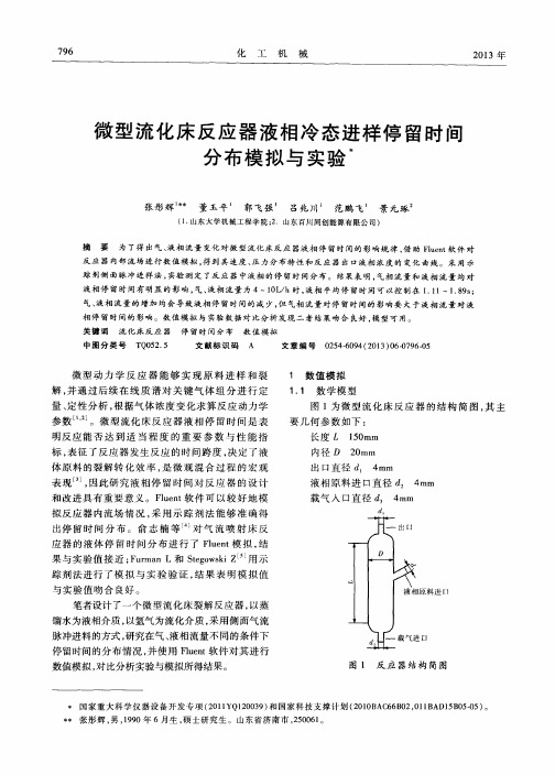
出 口直径 d 4 mm 液 相原料 进 口直径 d , 4 m m 载 气入 口直径 d 4 m m
出停 留时 间分 布 。俞 志 楠 等 对 气 流 喷 射床 反
7 9 8
化
工
机
械
2 0 l 3年
液相 流量 为 6 L / h时 , 不 同气 相 流 量 条 件 下
笔 者用下 式处 理 F l u e n t 模 拟结 果 , 得 到不 同
的停 留 时 间 分 布 曲 线 如 图 4所 示 ; 气 相 流 量 为
FLUENT流化床模拟实例

Tutorial:Using the Eulerian Multiphase Model with Species TransportIntroductionFluidized beds are used in processes where gas/solid mass transfer is of importance.The de-composition of ozone(O3),using particles as a catalyst,creates a suitable low-temperature environment for mass transfer.This tutorial solves a gas/solidflow with a simple one-step ozone decomposition reaction in afluidized bed.The reaction equation isO3→1.5O2(1) This tutorial demonstrates how to do the following:•Use the granular Eulerian multiphase model with species transport.•Define the rate of reaction with a user-defined function(UDF).•Define the Syamlal-O’Brien drag correlation with a user-defined function(UDF)usingappropriate parameters.•Set boundary conditions for internalflow.•Define thefluid and solid phases.•Calculate a solution using2D planar geometry in conjunction with the pressure-basedsolver.•Solve a time-accurate transient problem with data sampling for time statistics.PrerequisitesThis tutorial assumes that you are familiar with the FLUENT interface and that you have a good understanding of basic setup and solution procedures.Some steps will not be shown explicitly.In this tutorial you will use the Eulerian multiphase model with species transport.If you have not used this feature before,refer to the FLUENT6.3User’s Guide.Using the Eulerian Multiphase Model with Species TransportProblem DescriptionThe problem involves the transient startup of ozone decomposition in a fluidized bed.The fluid phase is a mixture of ozone and air,while the solid phase consists of sand particles with an 87.75micron diameter.A schematic of the fluidized bed is shown in Figure 1.The domain is modeled as a 2D planar cylindricalcase.volume fraction 0.52 of solids pressure outlet uniform velocity inlet u = 0.08 m/s 0 Pa gauge Figure 1:Problem SpecificationUsing the Eulerian Multiphase Model with Species Transport Preparation1.Copy thefiles2-D-FBed Ozone.msh.gz,rrate.c,and bp drag.c to your workingfolder.2.Start the2D double-precision(2ddp)version of FLUENT.Setup and SolutionStep1:Grid1.Read the gridfile(2-D-FBed_Ozone.msh).File−→Read−→Case...As FLUENT reads the gridfile,it will report its progress in the console.2.Check the grid.Grid−→CheckFLUENT will perform various checks on the mesh and will report the progress in the console.Make sure the minimum volume reported is a positive number.3.Display the grid using the default settings.Display−→Grid...Figure2:Grid Display4.Rotate the view so that the inlet of thefluidized bed is at the bottom.Display−→Views...Using the Eulerian Multiphase Model with Species Transport(a)Click the Camera...button to open the Camera Parameters panel.i.Drag the indicator of the dial with the left mouse button in the counter-clockwise direction until the upright view(-90◦)is displayed(Figure2).ii.Close the Camera Parameters panel.(b)Click the Save button in the Actions group box in the Views panel to save theupright view.When you do this,view-0will be added to the list of Views.(c)Close the Views panel.You can use the probe mouse button to check which zone number corresponds to eachboundary.If you click the probe mouse button on one of the boundaries in the graphicswindow,its zone number,name,and type will be printed in the FLUENT console.Thisfeature is especially useful when you have several zones of the same type and you wantto distinguish between them quickly.Using the Eulerian Multiphase Model with Species Transport Step2:Models1.Specify a transient,2D model.Define−→Models−→Solver...(a)Retain the default selection of Pressure Based from the Solver list and2D fromthe Space list.The pressure based solver must be used for multiphase calculations.(b)Select Unsteady from the Time list.(c)Click OK to close the Solver panel.2.Define the multiphase model.Define−→Models−→Multiphase...(a)Select Eulerian from the Model list.The panel will expand to show the inputs for the Eulerian model.Using the Eulerian Multiphase Model with Species Transport(b)Retain the default value of2for Number of Phases.(c)Click OK to close the Multiphase Model panel.3.Define the species model.Define−→Models−→Species−→Transport&Reaction...(a)Select Species Transport from the Model list.The Species Model panel will expand.(b)Enable Volumetric from the Reactions group box.(c)Disable Diffusion Energy Source from the Options group box.(d)Click OK to close the Species Model panel.Using the Eulerian Multiphase Model with Species Transport FLUENT will list the properties required for the models that you enabled,in theconsole.An Information dialog box will appear,reminding you to confirm theproperty values that have been extracted from the database.(e)Click OK in the Information dialog box to continue.Step3:MaterialsDefine−→Materials...1.Create a new material called air+ozone.(a)Click the Fluent Database...button to open the Fluent Database Materials panel.i.Selectfluid from the Material Type drop-down list.ii.Select ozone(o3)from the Fluent Fluid Materials selection list.iii.Click Copy to copy the information for ozone to your model and close the Fluent Database Materials panel.(b)Select mixture from the Material Type drop-down list.(c)Enter air+ozone for Name.(d)Click Change/Create.When you click Change/Create,a Question dialog box will appear,asking you ifmixture-template should be overwritten.Click No to retain mixture-template andadd the new material,air+ozone,to the list.The Materials panel will be updatedto show the new material name in the Fluent Mixture Materials list.Using the Eulerian Multiphase Model with Species Transport2.Click the Edit...button to the right of the Mixture Species drop-down list to open theSpecies panel.You will select the species that are involved in the decomposition of ozone.The orderof the species in the Selected Species list is important.Perform the following steps to achieve the proper order:(a)Select water-vapor(h2o)from the Selected Species selection list and click theRemove button to move it to the Available Materials selection list.(b)Similarly,remove n2from the Selected Species list.(c)Select ozone(o3)from the Available Materials selection list and click the Addbutton.(d)Similarly,add n2back in the Selected Species list.The Selected Species list should now contain o2,o3,and n2,respectively.(e)Click OK to close the Species panel.Using the Eulerian Multiphase Model with Species Transport 3.Click the Edit...button to the right of the Reaction drop-down list to open the Reac-tions panel.(a)Select o3from the Species drop-down list in the Reactants group box and enter1for both Stoich.Coefficient and Rate Exponent.(b)Select o2from the Species drop-down list in the Products group box and enter1.5for Stoich.Coefficient and0for Rate Exponent,respectively.There is no need to modify the Arrhenius Rate constants,as a UDF will be used to define them in Step4.(c)Click OK to close the Reactions panel.4.Retain the default settings in the Reaction Mechanisms panel.5.Select volume-weighted-mixing-law from the Density drop-down list.Thermal properties do not need to be specified since this is an isothermal case.6.Retain the default value of1.72e-05for Viscosity.7.Click Change/Create.Using the Eulerian Multiphase Model with Species Transport8.Create a new material called solids.In thefluidized bed the solid particles(treated as afluid)are held in suspension by theair+ozone mix injected at the bottom of the bed.(a)Selectfluid from the Material Type drop-down list.(b)Select water-vapor(h2o)from the Fluent Fluid Materials drop-down list.(c)Enter solids for Name.(d)Enter silica for Chemical Formula.(e)Enter2650kg/m3for Density.(f)Click Change/Create and close the Materials panel.When you click Change/Create,a question dialog box will appear,asking you ifwater-vapor(h2o)should be overwritten.Click No to retain water-vapor(h2o)and add the new material,solids,to the list.The Materials panel will be updatedto show the new material name in the Fluent Fluid Materials list.You can remove materials that are not required to run this case by selecting mix-ture in the Material Type in the Materials panel.Under Fluent Mixture Materials,select mixture-template from the drop-down list and click the Delete button.Simi-larly,selectfluid in the Material Type and delete all Fluent Mixture Materials otherthan O2,O3,N2,air and silica.9.Specify the species for the gaseous phase(phase-1)and the sand bed phase(phase-2).Define−→Models−→Species−→Transport&Reaction...(a)Select phase-1from the Phase drop-down list and click the Set...button to openthe Phase Properties panel.i.Select air+ozone from the Material drop-down list.ii.Click OK to close the Phase Properties panel.(b)Select phase-2from the Phase drop-down list and click the Set...button to openthe Phase Properties panel.i.Select solids from the Material drop-down list.ii.Click OK to close the Phase Properties panel.(c)Click OK to close the Species Model panel.Step4:User-Defined Functionspile the user-defined functions.Define−→User-Defined−→Functions−→Compiled...(a)Click the Add...button in the Source Files group box to open the Select Filepanel.(b)Select thefiles,rrate.c and bp drag.c and click OK.The bp drag.c source code is a routine for customizing the default Syamlal-O’Briendrag law in FLUENT.In the solid phase,the default drag law uses coefficientsof0.8(for voids≤0.85)and2.65(for voids>0.85),for minimumfluid ve-locities of0.25m/s.The current drag law has been modified to accommodate aminimumfluid velocity of0.08m/s.The source code,rrate.c,defines a customvolumetric reaction rate for the decomposition reaction of ozone.(c)Click Build to build the library.(d)Click Load to load the UDF.FLUENT will build a libudf folder and compile the UDF.A dialog box will appear warning you to make sure that UDF sourcefiles are inthe folder that contain your case and datafiles.Click OK in the dialog box.(e)Close the Compiled UDFs panel.2.Specify the volume reaction rate function.Define−→User-Defined−→Function Hooks...(a)Select rrate::libudf from the Volume Reaction Rate Function drop-down list.(b)Click OK to close the User-Defined Function Hooks panel.Step5:Phases1.Define the granular secondary phase.Define−→Phases...(a)Select phase-2and click the Set...button.i.Enable Granular.ii.Define the properties of the solid phase as shown in the table:Parameters ValuesDiameter8.775e-05mGranular Viscosity syamlal-obrienGranular Bulk Viscosity lun-et-alFrictional Viscosity schaefferAngle of Internal Friction30degreesGranular Temperature algebraicSolids Pressure syamlal-obrienRadial Distribution syamlal-obrienElasticity Modulus derivePacking Limit0.53Note:You will have to scroll down the Properties list to see the remaining options.iii.Click OK to close the Secondary Phase panel.2.Specify the drag law to be used for computing the interphase momentum transfer.(a)Click the Interaction...button to open the Phase Interaction panel.i.Select user-defined from the Drag Coefficient drop-down list to open the User-Defined Functions panel.A.Select custom drag syam::libudf and click OK to close the User-DefinedFunctions panel.ii.Click the Collisions tab and enter0.8for Constant Restitution Coefficient.iii.Click OK to close the Phase Interaction panel.3.Close the Phases panel.Step6:Operating ConditionsSet the gravitational acceleration.Define−→Operating Conditions...1.Enable Gravity.The panel will expand to show additional inputs.2.Enter-9.81m/s2for Gravitational Acceleration in the X direction.3.Enter297K for Operating Temperature.4.Click OK to close the Operating Conditions panel.Step7:Boundary ConditionsDefine−→Boundary Conditions...1.Set the conditions for the gaseous phase(phase-1).(a)Select Inlet from the Zone selection list.(b)Select phase-1from the Phase drop-down list and click the Set...button to openthe Velocity Inlet panel.i.Enter0.08m/s for Velocity Magnitude.ii.Click the Thermal tab and enter293K for Temperature.iii.Click the Species tab and enter0.2097and0.1for o2and o3respectively.iv.Click OK to close the Velocity Inlet panel.2.Define the boundary conditions for leftwall.(a)Select leftwall from the Zone selection list.(b)Select phase-2from the Phase drop-down list and click the Set...button to openthe Wall panel.i.Select Specularity Coefficient from the Shear Condition list and enter0.5forSpecularity Coefficient.ii.Click OK to close the Wall panel.3.Define the boundary conditions for the rightwall zone identical to that of the leftwall.4.Close the Boundary Conditions panel.Step8:AdaptionA small region will be adapted in order to create a register so that the solid volume fraction can be patched.1.Adapt the the regions to be patched.Adapt−→Region...(a)Enter0and0.115for X Min and X Max respectively.(b)Enter0and10for Y Min and Y Max respectively.(c)Click Mark.FLUENT will report the number of cells marked for adaption in the console.Clicking the Manage...button will open the Manage Adaption Registers panel.The name of the register created will be hexahedron-r0.(d)Close the Region Adaption panel.Step9:Solution1.Set the solution parameters.Solve−→Controls−→Solution...(a)Deselect Energy from the Equations selection list.(b)Enter0.7and0.3for Pressure and Momentum respectively.Note:You will have to scroll down Under-Relaxation Factors to see the remaining parameters.(c)Enter1.0for Granular Temperature.(d)Select Second Order Upwind from the Momentum,Energy,phase-1o2and phase-1o3drop-down lists.(e)Select QUICK from the Volume Fraction drop-down list.(f)Click OK to close the Solution Controls panel.2.Enable the plotting of residuals during the calculation.Solve−→Monitors−→Residual...3.Initialize the solution.Solve−→Initialize−→Initialize...(a)Change the initial phase-1X Velocity to0.01.(b)Change the initial phase-1o2to0.233(composition of oxygen in air).(c)Retain all other default initial values.(d)Click Init and close the Solutio Initialization panel.4.Patch the initial sand bed configuration.Solve−→Initialize−→Patch...(a)Select phase-2from the Phase drop-down list.(b)Select Volume Fraction from the Variable selection list.(c)Select hexahedron-r0from the Registers To Patch selection list.(d)Enter0.52for Value.(e)Click Patch and close the Patch panel.After initializing the entire domain of yourflowfield,you can enter different initial-ization values for particular variables into different cells.This is known as patching and is generally used if you have multiplefluid zones that you want to patch with different values.5.Set the time stepping parameters.Solve−→Iterate...(a)Enter0.001for Time Step Size and10000for Number of Time Steps.(b)Select Fixed from the Time Stepping Method list.(c)Enable Data Sampling for Time Statistics.This will allow you to sample data at a frequency that is set by you.(d)Enter40for Max Iterations per Time Step.(e)Click Apply.6.Save the initial case and datafiles(ozone fluidbed.cas.gz andozone fluidbed.dat.gz).File−→Write−→Case&Data...7.Save the datafiles every1000time steps.File−→Write−→Autosave...(a)Enter1000for Autosave Data File Frequency.(b)Enter ozonefluidbed%t.dat.gz for Filename.(c)Click OK to close the Autosave Case/Data panel.8.Click Iterate to run the calculation for10seconds in the Iterate panel.Step10:PostprocessingYou will now examine the progress of the sand and ozone/air mixture in thefluidized bed after a total of10seconds.Thefluidized bed should have reached a steadyflow solution at this time.1.Plot contours of mass fraction for oxygen and ozone species.Display−→Contours...(a)Select Species...and Mass fraction of o3from the Contours of drop-down list.(b)Enable Filled from the Options list.(c)Click Display.The O3mass fraction contours are shown in Figure3.(d)Similarly plot the mass fraction contours of O2.The mass fraction contours of O2is shown in Figures4.In Figure3you can see that O3is almost fully decomposed as it approaches the outlet of thefluidized bed.Figure3:O3Mass FractionFigure4:O2Mass Fraction2.View the phase motion by displaying plots of velocity vectors for the gas and solidphases.Display−→Vectors...(a)Select Velocity from the Vectors of drop-down list and phase-1from the Phasedrop-down lists.(b)Select Velocity...and Velocity Magnitude from the Color by drop-down list andphase-1from the Phase drop-down list.(c)Enter5for Scale and2for Skip to improve visualization of the velocity vectors.(d)Click Display.The phase-1velocity vectors are shown in Figure5.(e)Select phase-2from the Phase drop-down list to plot the phase-2velocity vectors.The phase-2velocity vectors are shown in Figure6.Figure5:Velocity Vectors for Phase-1Figure6:Velocity Vectors for Phase-23.Displayfilled contours of Phases...by Volume fraction for phase-1.Display−→Contours...(a)Select Phases...and Volume fraction from the Contours of drop-down list.(b)Select phase-1from the Phase drop-down list.(c)Click Display.The contours of volume fraction for phase-1are shown in Figure7.Figure7:Volume Fraction for Phase-1pare the mass fraction of O3and O2at the pressure outlet of thefluidized bed.Plot−→XY Plot...(a)Display an XY plot of mass fraction of O2.i.Select Species...and Mass fraction of o2from the Y Axis Function drop-downlist.ii.Retain the default selection of Direction Vector from the X Axis Function drop-down list.iii.Select outlet from the Surfaces selection list.iv.Enter0for X Plot Direction and1for Y Plot Direction.v.Click Plot.(b)Similarly,display an XY plot of mass fraction of O3by selecting Mass fraction ofo3from the Y Axis Function drop-down list.(c)Compare the O2and O3XY plots for mass fraction in Figure8and Figure9.Figure8:XY Plot of Mass Fraction of O3Figure9:XY Plot of Mass Fraction of O2SummaryThis tutorial demonstrated how to set up and solve a granular multiphase problem using the Eulerian multiphase model with species transport and reaction.The problem involved the2D modeling of particle suspension in afluidized bed,and postprocessing showed the near-steady-state behavior of the sand in thefluidized bed,under the assumptions made. Such cases should be typically run for a total of40seconds of operation,however,as this is very computationally intensive,this case was only run for10seconds for demonstration in this tutorial.。
流化床干燥综合3D虚拟仿真试验项目操作说明

流化床干燥综合3D虚拟仿真实验项目操作说明流化床干燥综合3D虚拟仿真实验项目是利用动态数学模型实时模拟真实实验流化床干燥的现象和过程,通过3D 仿真实验装置交互式操作,产生和真实实验相一致的实验现象和结果。
根据学生的需求与知识结构,构建了两个层次(基础理论型、仿真操作型)四个教学单元的实验内容,使实践教学内容由验证理论向综合应用、研究设计延伸,使不同层次、不同类型的学生都能在本仿真项目中,根据自己的需要来进行自主学习。
能够体现化工实验步骤和数据梳理等基本实验过程,满足工艺操作要求,满足流程操作训练要求,能够安全、长周期运行。
既能让每位学生都能亲自动手做实验,观察实验现象,记录实验数据,达到验证公式和原理的目的,且能够进一步通过对设备参数的改变,来加深对知识点和原理的理解。
一、干燥工艺及相关设备的认识本单元主要包括干燥工艺的主要原理、流程、设备及过程特点等,并拓展介绍相关的流体输送设备、传热流程及设备。
通过手动设备拆装,观察流化床干燥器内部构件,达到了解其整体结构的目的。
二、流化床干燥单元操作的开车、停车本单元的主要目的是让学生掌握流化床干燥单元的开、停车方法过程中所需要控制的相关参数等。
在这一单元,采用指导模式和自主操作两种学习方式。
指导模式的学习,是学生在软件提示下,进行设备的开停车步骤操作。
学生也可以选择自主操作模式,自主操作设备的开车、正常运行和停车步骤。
基本操作1、快捷键操作:W(前)S(后)A(左)D(右)、鼠标右键(视角旋转)。
图 1-1注:在非中文输入状态下,点击 W 可逐步放大页面,点击 A 界面右移,可使左边装置进入视角,点击 D 界面左移,可使右边装置进入视角,点击 S,退出拉近,界面恢复。
2、进入主场景后,可进入相应实验室,如流体力学实验室,完成实验的全部操作,进入实验室后可回到主场景中。
按住鼠标滚轮上下移动鼠标可进行视角的调整。
3、拉近镜头:鼠标左键双击设备进行操作,还可使用快捷键 W。
聚乙烯流化床反应器床内温度分布的模拟

聚乙烯流化床反应器床内温度分布的模拟聚乙烯是一种广泛应用的塑料,其生产过程中需要使用一些特殊的反应器,其中流化床反应器是一种常用的设备。
在流化床反应器中,聚乙烯颗粒被加热至高温,然后通过催化剂进行反应,最终形成聚乙烯产品。
在这个过程中,反应器床内的温度分布对反应的效率和产品质量都有着重要的影响。
因此,模拟反应器床内温度分布是一个非常重要的课题。
本文将介绍聚乙烯流化床反应器床内温度分布的模拟方法和结果。
首先,我们将介绍流化床反应器的基本原理和反应机理。
然后,我们将详细介绍模拟方法,包括数值模拟的基本原理和计算流体力学(CFD)模拟方法。
最后,我们将呈现模拟结果,并对结果进行分析和讨论。
一、流化床反应器的基本原理和反应机理流化床反应器是一种将反应物料放在气体流动中进行反应的设备。
在流化床反应器中,催化剂通常被放置在一个床层中,并被气体携带到反应物料中进行反应。
在聚乙烯生产中,反应物料通常是乙烯气体,而催化剂则是一种Ziegler-Natta催化剂。
聚乙烯的反应机理比较复杂,但可以简单地概括为以下几个步骤:1. 乙烯气体被吸附在催化剂表面。
2. 催化剂与乙烯气体反应,形成聚合物链。
3. 聚合物链不断生长,直到达到一定长度。
4. 聚合物链脱离催化剂表面,成为自由的聚合物。
5. 自由的聚合物不断生长,直到形成聚乙烯颗粒。
在这个过程中,床层内的温度对反应的速率和产物的质量都有着非常重要的影响。
二、模拟方法1. 数值模拟的基本原理数值模拟是一种通过计算机模拟物理现象的方法。
在模拟过程中,将物理现象分割成许多小的区域,并在每个区域中进行计算。
这种方法可以帮助我们更好地理解物理现象,并预测未来的变化。
2. 计算流体力学(CFD)模拟方法计算流体力学(CFD)是一种通过计算机模拟流体力学现象的方法。
在CFD模拟中,将流体分割成小的区域,并在每个区域中进行计算。
这种方法可以帮助我们更好地理解流体力学现象,并预测未来的变化。
灰熔聚流化床气化炉内气固两相流的数值模拟
传热 的传 质机 理 的关 键 , 提 高 I C效 率及 碳 转化 对 C
率有着 重要意 义. 研究基 于 欧拉双 流体模 型 , 本 利用
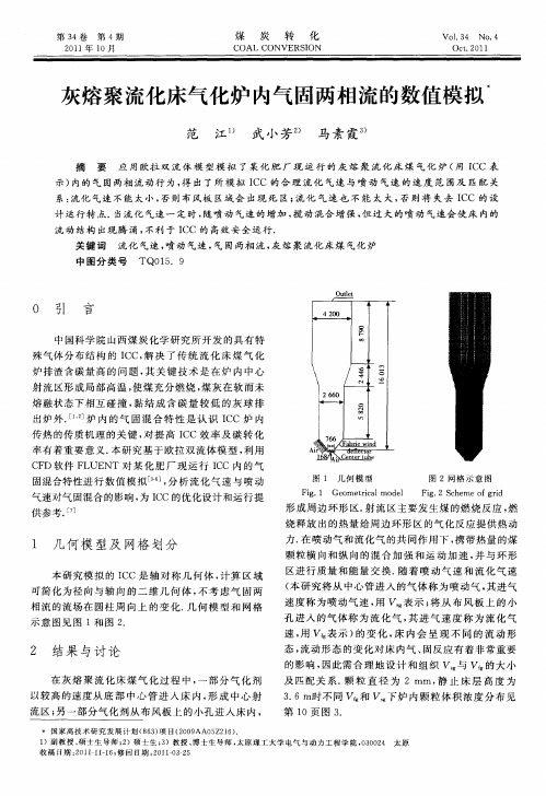
C D软件 F NT对 某 化肥 厂 现 运 行 IC 内的 气 F I UE C 固混合特性进行 数 值模 拟¨6, 析流 化气 速 与喷 动 3】分 _ 气速对气 固混 合的影响 , IC的优化设计 和运行 提 为 C
供参考. ] f
图 1 几 何 模 型
Fi .1 Ge g om e rc lm ode tia l
1 )副 教授 、 士 生 导 师 ;)硕 士 生 ;)教 授 、 士 生 导 师 , 原 理 工 大 学 电 气 与 动 力工 程 学 院 ,3 0 4 太 原 硕 2 3 博 太 002 收 稿 日期 :o l1一6 修 回 日期 :O i0 5 2 l l1 ; 2 1-32
1 2
5m/ , 于 2 s 合 理 的 Vf , 存 在 一 最 佳 s小 5 m/ . g 必 下 V , 炉 内气 体 分 布结 构满 足 I C要 求 , 使 C 且气 固混
合效果 最好. 一 结论 不 会 随静 止床 层 高 度 的变 化 这
0 引 言
中国科 学 院山西 煤炭化 学研究 所开 发 的具 有特 殊气 体分 布结 构 的 I C, C 解决 了传 统 流 化床 煤 气 化 炉排 渣含碳 量 高的 问题 , 其关 键 技术 是 在 炉 内 中心
射流 区形成 局部 高温 , 煤充 分燃烧 , 使 煤灰 在软 而未
示) 内的 气 固 两相 流 动 行 为 , 出 了所 模 拟 I C 的 合 理 流 化 气 速 与 喷 动 气 速 的 速 度 范 围 及 匹 配 关 得 C 系 : 化 气 速 不 能 太 小 , 则 布 风 板 区域 会 出现 死 区 ; 化 气 速 也 不 能 太 大 , 则 将 失 去 I C 的 设 流 否 流 否 C
循环流化床烟气脱硫塔内气液两相流场数值模拟
Absr t:I h sp p r, a —i u d t — h s o fed o ic l t u d z d b d f a s lu z to o t ac n t i a e g slq i wo p a ef w l fcr u a i f i ie e ueg sde u f r ai n tw— l i ngl l i
环流化床脱硫技术进行进一步研究有重要的意义。影响循环流化床脱硫率 的最大因素之一就是气液固 三相是否能够有效均匀的混合反应 [ 。本文是以某热 电有限公司所使用的循环流化床脱硫塔为研究 5 ] 对象 , 采用 F U N L E T软件来模拟脱硫塔内部流场的变化情况 , 主要是关注于气液两相流 , 不考虑固体脱 硫 剂 的喷人 情 况 , 只考 虑被 处理 烟气 与雾化 水混合 的流 场情 况 , 即不 带 化学 反应 的气 液 两相 流 动 …。
7 一7 O 6.
[ ] S unc e , i hoJ nu u n t . xe m na s d nFu a eup ui t nb i uan udzdbd[ . rce ig 7 h agh nMa Y a ,ajnH age a E pr e t t yo legs slh rai ycr lt gf ii e C] Poedns Z i 1 i lu d z o c i l e
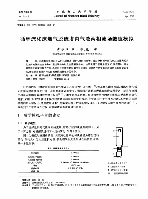
简化 , 烟气 入 口为文 丘里 扩 充段 , 设 烟气在 文 丘里 段 已经 流动 均 匀 。 假 基 本 参数如 下 :
6
表 1 脱硫 塔 简 化 后 尺 寸
塔体直径 文丘里下端直径 文丘里扩充段高 烟 气 出 口( 形 ) 矩 塔 高
喷 嘴 布 置
62 o mm 0
e s su id b u r a i lt n T e v l ct i r u i n a d tmp r t r e d d s b t n a d t r u rwa t d e y n me c ls i mu ai . h eo i d s b t n e e a u e f l it u i n u b 一 o y t i o i i r o 1n n e s y d sr u in w sa ay e l n h e g to i u ai g f i ie e . h e u t s o e h e ti s n i it b t a n z d ao g t e h ih f r lt u d z d b d T e r s l h w wh n t e t i o l c c n l s n zl sd c r td a n l 4 f s i go el f w l wa ea iey s r u . h ih t mp r tr u a i o ze i e o ae t ge 5, u h n f h t al sr l t l e i s T eh g a l t e v o e e au ef e g sd d l
- 1、下载文档前请自行甄别文档内容的完整性,平台不提供额外的编辑、内容补充、找答案等附加服务。
- 2、"仅部分预览"的文档,不可在线预览部分如存在完整性等问题,可反馈申请退款(可完整预览的文档不适用该条件!)。
- 3、如文档侵犯您的权益,请联系客服反馈,我们会尽快为您处理(人工客服工作时间:9:00-18:30)。
大蒸馏渣油及罐区来混合蜡油(原料油)进入装置原料油罐(V-2101),后经原料油泵(P-2101A/B)升压,依次与分馏中段油(E-2101)、油浆(E-2102)换热后,与回炼油混合,从原料油雾化喷嘴进入提升管反应器(T-1101)反应区,与经蒸汽预提升的650~680℃左右的高温催化剂接触汽化并进行反应,反应油气经粗旋进行气剂粗分离,分离出的油气经单级旋分进一步脱除催化剂细粉后经大油气管线至分馏塔(T-2101)。
分离出的待生催化剂经沉降器汽提段汽提,汽提后的待生催化剂经待生催化剂滑阀、待生斜管,通过二次提升后至第二再生器(T-1104)。
待生催化剂在主风的作用下进行逆流烧焦,催化剂在680℃的条件下进行完全再生。
烧掉绝大部分的焦炭,烧焦产生的烟气,先经一、二级旋风分离器分离其中携带的催化剂,再经三级旋风分离器(V-1102)进一步分离催化剂后,高温烟气进入烟气轮机(C-1201)膨胀作功,驱动主风机组(C-1202)。
烟气出烟气轮机后,进入余热锅炉(F-1301),产生蒸汽,烟气经脱硫塔(T-1301)脱硫后排入大气。
再生催化剂经外取热器(E-1101)取走烧焦过程中产生的过剩热量,冷却的催化剂沿外取热器下滑阀返回再生器(T-1103)继续烧焦。
烧焦后的再生催化剂经再生斜管及再生滑阀至提升管预提升段。
在提升管预提升段,以蒸汽作提升介质,完成再生催化剂加速、整流过程,然后与雾化原料接触反应。