Ch3_Labor Demand 鲍哈斯劳动经济学

合集下载

劳动经济学课件(全) 第三章劳动力需求

希克斯技术进步资本密集型技术进步劳动密集型技术进步
劳动经济学
31
人力资源管理专业
第三节企业长期劳动力需求
四、劳动力需求变化
（三）政府的特殊政策
特殊就业促进政策发放工资补贴最低工资法
劳动经济学
32
人力资源管理专业
第三节企业长期劳动力需求
五、劳动力需求的调整
（一）生产规模的扩大
L
劳动经济学
24
人力资源管理专业
第三节企业长期劳动力需求
三、最佳生产方法与劳动力需求决定
（一）总成本既定
劳动经济学
25
人力资源管理专业
第三节企业长期劳动力需求
三、最佳生产方法与劳动力需求决定
（二）总产量既定
劳动经济学
26
人力资源管理专业
第三节企业长期劳动力需求
三、最佳生产方法与劳动力需求决定
复习思考：
1. 劳动力需求弹性 2. 企业短期劳动力需求 3. 企业长期劳动力需求
劳动经济学
35
人力资源管理专业
第一节劳动力需求概述
劳动力需求曲线 (labor demand curve)
W
0
劳动经济学
D
L
36
人力资源管理专业
第三节企业长期劳动力需求
某企业的产量可以表达为：
Q= f (L,K) = L K
企业使用机器的成本为 750 元 / 周，人力成本为 300元/周。当企业产量为1000单位时，确定企业最佳人力与资本组合。
当人力成本下降为225元/周时，确定企业最佳人力与资本组合，并计算劳动力需求弹性。
劳动经济学

《劳动经济学》(作者Borjas)第五章习题答案

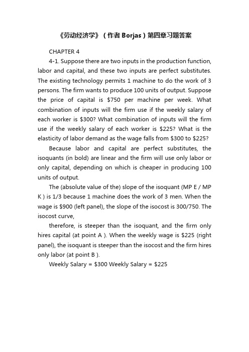
CHAPTER 55-1. Suppose the labor supply curve is upward sloping and the labor demand curve is downward sloping. The study of economic trends over a particular time period reveals that the wage recently fell while employment levels rose. Which curve must have shifted and in which direction to produce this effect?If the supply curve does not shift, all wage and employment movements must occur along the supply curve, so that the wage rate and the employment level must move in the same direction. Because the wage went down while employment went up in the situation described in the question, it must have been the case that the supply curve shifted outwards (to the right). We do not have enough information to determine whether the demand curve shifted as well.5-2. It takes time to produce a new economist, and prospective economists base their career decision by looking only at current wages across various professions. Further, the labor supply curve of economists is much more elastic than the labor demand curve. Suppose the market is now in equilibrium, but that the demand for economists suddenly rises because a new activist government in Washington wants to initiate many new programs that require the input of economists. Illustrate the trend in the employment and wages of economists as the market adjusts to this increase in demand.Initially, the market is in equilibrium at a wage w0 and an employment level of E0. The increase the demand for economists results in a new equilibrium wage of w1 and a new equilibrium employment level of E1. However, the demand for economists in the short-run is inelastic at E0, so the demand increase simply leads to a rise in the wage of economists (as indicated by point 1). In the next period, students believe this wage will persist and oversupply the market so that the cobweb leads to a new wage at point 2. In the next period, students undersupply (because the wage is too low) and the cobweb leads to a new wage at point 3, and so on. Because of the relative elasticities of supply and demand (as drawn), the cobweb is exploding and will never converge to a stable equilibrium.5-3. Suppose the supply curve of physicists is given by w = 10 + 5E , while the demand curve is given by w = 50 – 3E . Calculate the equilibrium wage and employment level. Suppose now that the demand for physicists increases and the new demand curve is given by w = 70 – 3E . Assume this market is subject to cobwebs. Calculate the wage and employment level in each round as the wage and employment levels adjust to the demand shock. (Recall that each round occurs on the demand curve – when the firm posts a wage and hires workers). What is the new equilibrium wage and employment level?The initial equilibrium is given by 10 + 5E = 50 – 3E . Solving these two equations simultaneously implies that w = $35 and E S = E D = 5. When demand increases to w = 70 – 3E , the new equilibrium wage is $47.5 and the equilibrium level of employment is 7.5.Round Wage Employment1 $55.0 52 $43.0 93 $50.2 6.64 $45.9 8.05 $48.4 7.26 $46.9 7.77 $47.8 7.48 $47.2 7.6The table gives the values for the wage and employment levels in each round. The values in the table are calculated by noting that in any given period the number of physicists is inelastically supplied, so that the wage is determined by the demand curve. Given this wage, the number of economists available in the next period is calculated. By round 7, the market wage rate is within 30 cents of the new equilibrium.01 w 1w 0W age5-4. The 1986 Immigration Reform and Control Act (IRCA) made it illegal for employers in the United States to knowingly hire illegal aliens. The legislation, however, has not reduced the flow of illegal aliens into the country. As a result, it has been proposed that the penalties against employers who break the law be increased substantially. Suppose that illegal aliens, who tend to be less skilled workers, are complements with native workers. What will happen to the wage of native workers if the penalties for hiring illegal aliens increase?A substantial increase in the penalties associated with hiring illegal aliens will likely reduce the number of illegal aliens entering the United States. The effect of this shift in the size of the illegal alien flow on the marginal product (and hence the demand curve) of native workers hinges on whether illegal aliens are substitutes or complements with natives. As it is assumed that natives and illegal aliens are complements, a cut in the number of illegal aliens reduces the value of the marginal product of natives, shifting down the demand for native labor, and decreasing native wages and employment.5-5. Suppose a firm is a perfectly discriminating monopsonist. The government imposes a minimum wage on this market. What happens to wages and employment?A perfectly discriminating monopsonist faces a marginal cost of labor curve that is identical to the supply curve. As a result, the employment level of a perfectly discriminating monopsonist equals theemployment level that would be observed in a competitive market (at E *) The imposition of a minimum wage at w MIN leads to the same result as in a competitive market: the firm will only want to hire E D workers as w MIN is now the marginal cost of labor, but E S workers will want to find work at the minimum wage. Thus, the wage increases, but employment falls.DollarsE w w *S D5-6. What happens to wages and employment if the government imposes a payroll tax on amonopsonist? Compare the response in the monopsonistic market to the response that would have been observed in a competitive labor market.Initially, the monopsonist hires E M workers at a wage of w M . The imposition of a payroll tax shifts the demand curve to VMP ′, and lowers employment to E ′ and the wage to w ′. Thus, the effect of imposing a payroll tax on a monopsonist is qualitatively the same as imposing a payroll tax in a competitive labor market: lower wages and employment. (It is interesting to note that the same result comes about if the payroll tax is placed on workers, so that the labor supply and marginal cost of labor curves shift as opposed to labor demand.)5-7. An economy consists of two regions, the North and the South. The short-run elasticity of labor demand in each region is –0.5. The within-region labor supply is perfectly inelastic. The labormarket is initially in an economy-wide equilibrium, with 600,000 people employed in the North and 400,000 in the South at the wage of $15 per hour. Suddenly, 20,000 people immigrate from abroad and initially settle in the South. They possess the same skills as the native residents and also supply their labor inelastically.(a) What will be the effect of this immigration on wages in each of the regions in the short run (before any migration between the North and the South occurs)?There will be no effect on the North’s labor supply in the short run, so the wage rate will not change there. In the South, labor supply will have increased by 5 percent, so the wage rate must fall by 5/(0.5) = 10 percent (recall that the elasticity of labor demand is -0.5, so a one percent decrease in wages would have been generated by a 0.5 percent expansion of the labor supply). The new hourly wage in the South, therefore, is $13.50 and total employment in the South is 420,000.DollarsEmploymentw M w ′(b) Suppose 1,000 native-born persons per year migrate from the South to the North in response to every dollar differential in the hourly wage between the two regions. What will be the ratio of wages in the two regions after the first year native labor responds to the entry of the immigrants?After the initial migration, we have seen that wages in the South are $13.50 while wages in the North are $15. This difference leads 1,500 natives migrating from the South to the North in the first year. Employment in the North after one year, therefore is 601,500. Moreover, as the elasticity of labor demand in the North is -0.5 and employment has increased by 0.25 percent, the Northern wage falls by 0.5 percent to roughly $14.93. Likewise, employment in the South after one year is 418,500. As the elasticity of labor demand is -0.5 and employment has decreased by 0.3571 percent, the Southern wage increases by0.71428 percent to roughly $13.60. Thus, the ratio of the Northern to Southern wage after one year is1.09779.(c) What will be the effect of this immigration on wages and employment in each of the regions in the long run (after native workers respond by moving across regions to take advantage of whatever wage differentials may exist)? Assume labor demand does not change in either region.In the long run, people must move from the South to the North to equalize the wage rates in the two regions. Since the wages were equal in the two regions before the influx of immigrants, and they also must be equal after things settle down, the proportional decrease in the wage rate should be the same in the North and in the South. Because the elasticity of labor demand is the same in the two regions, this last observation implies that the percentage increase in employment in the North must be the same as the percentage increase in employment in the South. Thus, as 60 percent of the original workers were employed in the North, 60 percent of the 20,000 increase in Southern employment will eventually migrate to the North. In the long run, therefore, total Northern employment will be 612,000 while total Southern employment will be 408,000. (Note: there is no presumption that only immigrants further migrate to the North.) In each region, therefore, employment increases by 2 percent in the long run, i.e., 12,000 is 2 percent of 600,000 and 8,000 is 2 percent of 400,000. (This can also be seen immediately as 20,000 is 2 percent of the 1 million workers.) Now, given that the elasticity of labor demand is -0.5, the 2 percent increase in employment will cause the wage rate to fall by 4 percent. Hence, the long-run equilibrium hourly wage will be $14.40.5-8. Chicken Hut faces perfectly elastic demand for chicken dinners at a price of $6 per dinner. The Hut also faces an upward sloped labor supply curve ofE = 20w – 120,where E is the number of workers hired each hour and w is the hourly wage rate. Thus, the Hut faces an upward sloped marginal cost of labor curve ofMC E = 6 + 0.1E.Each hour of labor produces 5 dinners. (The cost of each chicken is $0 as the Hut receives two-day old chickens from Hormel for free.) How many workers should Chicken Hut hire each hour to maximize profits? What wage will Chicken Hut pay? What are Chicken Hut’s hourly profits?First, solve for the labor demand curve: VMP E = P x MP E = $6 x 5 = $30. Thus, every worker is valued at $30 per hour by Chicken Hut. Now, setting VMP E = MC E yields 30 = 6 + .1E which implies E* = 240. Thus, Chicken Hut will hire 240 workers every hour. Further, according to the labor supply curve, 240 workers can be hired at an hourly wage of $18. Finally, Chicken Hut’s profits are Π = 240(5)($6) –240($18) = $2,880.5-9. Polly’s Pet Store has a local monopoly on the grooming of dogs. The daily inverse demand curve for pet grooming is:P = 20 – 0.1Qwhere P is the price of each grooming and Q is the number of groomings given each day. This implies that Polly’s marginal revenue is:MR = 20 – 0.2Q.Each worker Polly hires can groom 20 dogs each day. What is Polly’s labor demand curve as a function of w, the daily wage that Polly takes as given?As each worker can groom 20 dogs each day, and using Q = 20E, we have thatVMP E = MR x MP E = ( 20 – 0.2Q ) (20) = (20 – 4E)(20) = 400 – 80E.Thus, as Polly’s demand for labor satisfies VMP E = w, we have that her labor demand curve isE = 5 – 0.0125w.5-10. The Key West Parrot Shop has a monopoly on the sale of parrot souvenir caps in Key West. The inverse demand curve for caps is:P = 30 – 0.4 Qwhere P is the price of a cap and Q is the number of caps sold per hour. Thus, the marginal revenue for the Parrot Shop is:MR = 30 – 0.8Q.The Parrot Shop is the only employer in town, and faces an hourly supply of labor given by:w = 0.9E + 5where w is the hourly wage rate and E is the number of workers hired each hour. The marginal cost associated with hiring E workers, therefore, is:MC E = 1.8E + 5.Each worker produces two caps per hour. How many workers should the Parrot Shop hire each hour to maximize its profit? What wage will it pay? How much will it charge for each cap?First, as Q = 2E, the labor demand curve isVMP E = MR x MP E = (30 – 0.8Q)(2) = 60 – 1.6Q = 60 – 3.2E.Setting VMP E equal to MC E and solving for E yields E = 11. Eleven workers can be hired at a wage of.9(11) + 5 = $14.99 per hour. The 11 workers make 22 caps each hour, and the 22 caps can be sold at a price of 30 – 0.4(22) = $21.20 each.5-11. Ann owns a lawn mowing company. She has 400 lawns she needs to cut each week. Her weekly revenue from these 400 lawns is $20,000. If given an 18-inch deck push mower, a low-skill worker can cut each lawn in two hours. If given a 60-inch deck riding mower, a low-skill worker can cut the lawn in 30 minutes. Low-skilled labor is supplied inelastically at $5.00 per hour. Each laborer works 8 hours a day and 5 days each week.(a) If Ann decides to have her workers use push mowers, how many push mowers will Ann rent and how many workers will she hire?As each worker can cut a lawn in 2 hours, it follows that each worker can cut 4 lawns in a day or 20 lawns in a week. Therefore, Ann would need to rent 20 push mowers and hire 20 workers in order to cut all 400 lawns each week.(b) If she decides to have her workers use riding mowers, how many riding mowers will Ann rent and how many workers will she hire?As each worker can cut a lawn in 30 minutes, it follows that each worker can cut 16 lawns in a day or 80 lawns in a week. Therefore, Ann would need to rent 5 riding mowers and hire 5 workers in order to cut all 400 lawns each week.(c) Suppose the weekly rental cost (including gas and maintenance) for each push mower is $250 and the weekly rental cost (including gas and maintenance) of each riding mower is $1,800. What equipment will Ann rent? How many workers will she employ? How much profit will she earn?If Ann uses push mowers, her weekly cost of mowers is $250(20) = $5,000 while her weekly labor cost is $5(20)(40) = $4,000. Under this scenario, her weekly profit is $11,000. If Ann uses riding mowers, her weekly cost of mowers is $1,800(5) = $9,000 while her weekly labor cost is $5(5)(40) = $1,000. Thus, under this scenario, her weekly profit is $10,000. Therefore, under these conditions, Ann will rent 20 push mowers and employ 20 low-skill workers.(d) Suppose the government imposes a 20 percent payroll tax (paid by employers) on all labor and offers a 20 percent subsidy on the rental cost of capital. What equipment will Ann rent? How many workers will she employ? How much profit will she earn?Under these conditions, the cost of labor has increased to $6.00 per hour, while the rental costs for a push mower and a riding mower have decreased to $200 and $1,440 respectively. Ann’s profits under the two options, therefore, arePush-Profit = $20,000 – $200(20) – $6(20)(40) = $11,200.Rider-Profit = $20,000 – $1,440(5) – $6(5)(40) = $11,600.Thus, under these conditions, Ann rents riding mowers, hires 5 low-skill workers, and earns a weekly profit of $11,600.5-12. In the United States, some medical procedures can only be administered to a patient by a doctor while other procedures can be administered by a doctor, nurse, or lab technician. What might be the medical reasons for this? What might be the economic reasons for this?The American Medical Association might argue that doctors have more training and experience than nurses, and therefore, are the only professionals who can make certain decisions or perform certain procedures.Economically, the AMA has an incentive to restrict the number of people who can practice medicine (or perform certain procedures) in order to keep doctor wages high. If nurses were allowed to do everything they were capable of, fewer doctors would be demanded, and doctor wages would fall. From an economic viewpoint, therefore, the AMA restricts the supply of doctors, which keeps doctor wages artificially high.WageW restW unrestRestricted Supply ofDoctorsUnrestricted Supplyof DoctorsL rest L unrest Services Provided by DoctorsLabor Market For Medical Services Provided by Doctors。

劳动经济学第四章劳动力需求

劳动经济学第四章劳动力需求劳动经济学是研究劳动市场及其与经济系统相互作用的学科。

在劳动分工和劳动力的需求方面，劳动经济学提供了深入的理论和实证研究。

本文将聚焦于劳动经济学中的第四章——劳动力需求，探讨劳动力需求的决定因素和影响机制。

一、劳动力需求的概念及决定因素劳动力需求是指企业或机构对劳动力数量的需求，涉及到劳动人口的就业。

劳动力需求决定因素复杂多样，主要包括以下几个方面:1. 经济增长率：经济增长率对劳动力需求产生直接影响。

经济增长率高的国家或地区，企业投资扩张、产业发展迅速，因此对劳动力的需求也相对较大。

2. 劳动生产率：劳动生产率是决定劳动力需求的重要因素。

生产力水平高的企业可以通过单位劳动力的数量实现较高的产出，因此对劳动力的需求相对较少。

3. 技术进步与创新：技术进步和创新对劳动力需求产生深远影响。

高新技术行业的发展往往需要更多的技术人才，因此对劳动力的需求也随之增加。

4. 政府政策与法规：政府对劳动力市场的干预也是劳动力需求的决定因素之一。

政府的就业政策、劳动法规等都会直接或间接影响企业对劳动力的需求。

二、劳动力需求的影响机制1. 边际产品与边际成本理论：企业在决定是否雇佣额外劳动力时，会比较劳动力的边际产品与边际成本。

当边际产品大于边际成本时，企业会继续增加劳动力；当边际产品小于边际成本时，企业会减少劳动力。

2. 调整成本与规模效应：调整成本是指企业在改变雇佣劳动力数量时所需要支付的成本，主要包括流动性成本和固定成本。

规模效应是指企业规模对单位产品成本的影响。

当企业规模扩大时，单位产品成本往往会下降。

3. 劳动力替代与辅助技术：某些劳动力可以被机器或技术所替代，特别是一些重复性和繁重的劳动岗位。

而对于一些需要辅助技术或专业技能的职位，劳动力需求相对较高。

4. 资本与劳动力替代：在生产过程中，企业可以通过增加资本投入来替代一部分劳动力。

当资本相对便宜或劳动力相对昂贵时，企业更倾向于选择资本替代劳动力。

劳动经济学(鲍哈斯版)重点复习题总结

第四章
1.论述一个存在着两部门的经济中，最低工资对被覆盖的部门和未被覆盖的部门的影响。（P175）
答：（P154）（图）
如果到最低工资仅仅在被覆盖部门的工作岗位上推行，那么被替代的工作者也许就会移动到未被覆盖的部门，以至供给曲线会向右移动，减少为被覆盖部门的工资。如果获得最低工资工作岗位是容易的，那么在未被覆盖部门工作的工作者也许就会辞去他们的工作，在被覆盖的部门等待，直到一个工作岗位出现，将未被覆盖部门的供给曲线移动到左边，并且提高未被覆盖部门的工资。
第三章
1.什么是新增工作者效应？什么是受阻工作者效应？（P107）
答：
（1）新增工作者效应：指在经济衰退时期由于家中主要劳动力失去工作（家庭收入下降），次级劳动者不得不寻找工作弥补家庭收入损失。因此新增工作者效应意味着次级劳动力参与率具有一种逆（反）周期趋势。
（2）受阻工作者效应：a.指很多失业者在衰退时期感觉找不到工作，于是干脆放弃了（暂时退出）；b.隐性失业者——存在受阻工作者效应的结果是劳动参与率具有一种顺应周期趋势。
第十章
1.劳动力市场歧视（论述题）：（P444）
答：
Ⅰ.个人偏好性歧视：
构成
利润
雇佣人数
雇主歧视
纯（黑白分明）
↓
↓
雇员歧视
纯（黑白分明）
不变
↓
顾客歧视
①能藏：不分
不变
不变
②不可藏：纯白人
不变
不变
Ⅱ.统计性歧视：来自于群体
素质越高，越遭歧视；反之—
2.请推倒瓦哈卡歧视测度方法。这种统计方法真的能测度歧视对受影响群体的相对工资的影响吗？（P444）（计算题）
（1）女性真实工资的明显提高；
（2）生育行为的变化：①生育观念变化（不愿生）；②市场工资的提高也使得抚养孩子成为一种昂贵的家庭活动，因而成为家中孩子数减少的原因之一——③致使妇女的保留工资的下降，更愿意进入劳动力市场；

《劳动经济学》（作者Borjas）第四章习题答案

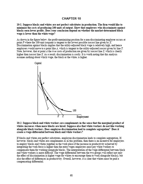
《劳动经济学》（作者Borjas）第四章习题答案CHAPTER 44-1. Suppose there are two inputs in the production function, labor and capital, and these two inputs are perfect substitutes. The existing technology permits 1 machine to do the work of 3 persons. The firm wants to produce 100 units of output. Suppose the price of capital is $750 per machine per week. What combination of inputs will the firm use if the weekly salary of each worker is $300? What combination of inputs will the firm use if the weekly salary of each worker is $225? What is the elasticity of labor demand as the wage falls from $300 to $225?Because labor and capital are perfect substitutes, the isoquants (in bold) are linear and the firm will use only labor or only capital, depending on which is cheaper in producing 100 units of output.The (absolute value of the) slope of the isoquant (MP E / MP K ) is 1/3 because 1 machine does the work of 3 men. When the wage is $900 (left panel), the slope of the isocost is 300/750. The isocost curve,therefore, is steeper than the isoquant, and the firm only hires capital (at point A ). When the weekly wage is $225 (right panel), the isoquant is steeper than the isocost and the firm hires only labor (at point B ).Weekly Salary = $300 Weekly Salary = $225The elasticity of labor demand is defined as the percentage change in labor divided by the percentage change in the wage. Because the demand for labor goes from 0 to a positive quantity when the wagedropped to $225, the (absolute value of the) elasticity of labor demand is infinity.LaborCapitalLaborCapital4-2. (a) What happens to the long-run demand curve for labor if the demand for the firm’s output increases?The labor demand curve is given by VMP E = MR x MP E. As demand for the firm’s output increases, its marginal revenue also increases. Thus, an increase in demand for the firm’s output shifts the labor demand curve to the right.(b) What happens to the long-run demand curve for labor if the price of capital increases?To determine how an increase in the price of capital changes the demand for labor, suppose initially that the firm is producing 200 units of output at point P in the figure. The increase in the price of capital (assuming capital is a normal input) increases the marginal costs of the firm and will reduce the profit-maximizing level of output to say 100 units. The increase in the price of capital also flattens the isocost curve, moving the firm to point R. The move from point P to point R can be decomposed into a substitution effect (P to Q) which reduces the demand for capital, but increases the demand for labor, and a scale effect (Q to R) which reduces the demand for both labor and capital. The direction of the shift in the demand curve for labor, therefore, will depend on which effect is stronger: the scale effect or the substitution effect.4-3. Union A wants to represent workers in a firm that hires 20,000 person workers when the wage rate is $4 and hires 10,000 workers when the wage rate is $5. Union B wants to represent workers in a firm that hires 30,000 workers when the wage is $6 and hires 33,000 workers when the wage is $5. Which union would be more successful in an organizing drive?The union will be more likely to attr act the workers’ support when the elasticity of labor demand (in absolute value) is small. The elasticity of labor demand facing union A is given by: η = percent ?L / percent ?w = (20,000–10,000)/20,000 ÷ (4–5)/4 = –2.The elasticity of labor demand facing union B equals (33,000–30,000)/33,000 ÷ (5–6)/5 = –5/11 ≈ –.45. Union B, therefore, is likely to have a more successful organizing drive as 0.45 < 2.4-4. Consider a firm for which production depends on two normal inputs, labor and capital, with prices w and r, respectively. Initially the firm faces market prices of w = 6 and r = 4. These prices then shift to w = 4 and r = 2.(a) In which direction will the substitution effect change the firm’s employment and capital stock?Prior to the price shift, the absolute value of the slope of the isocost line (w/r) was 1.5. After the price shift, the slope is 2. In other words, labor has become relatively more expensive than capital. As a result, there will be a substitution away from labor and towards capital (the substitution effect).(b) In which direction will the scale effect change the firm’s employment and capital stock?Because both prices fall, the marginal cost of production falls, and the firm will want to expand. The scale effect, therefore, increases the demand for both labor and capital (as both are normal inputs).(c) Can we say conclusively whether the firm will use more or less labor? More or less capital?The firm will certainly use more capital as the substitution and scale effects reinforce each other in that direction, but the change in labor employed will depend on whether the substitution or the scale effect for labor dominates.4-5. What happens to employment in a competitive firm that experiences a technology shock such that at every level of employment its output is 200 units/hour greater than before?Because output increases by the same amount at every level of employment, the marginal product of labor, and hence the value of the marginal product of labor, does not change. Therefore, as the value of the marginal product of labor will equal the wage rate at the same level of employment as before, the level of employment will not change.4-6. Suppose the market for labor is competitive and the supply curve for labor is backwardbending over part of its range. The government now imposes a minimum wage in this labor market. What is the effect of the minimum wage on employment? Does the answer depend on which of the two curves (supply or demand) is steeper? Why?Equilibrium is attained where the supply curve intersects the demand curve, and the equilibriumemployment and wage levels are E* and w*, respectively . When the minimum wage is set at w MIN , the firm wants to hire E D workers but E S workers are looking for work. As long as the downward-sloping portion of the supply curve is to the right of the demand curve, the fact that the supply curve is downward sloping creates no problems beyond those encountered in the typical competitive model. An interesting extension of the problem would consider the case where the downward-sloping portion of the supply curve recrosses the demand curve at some point above w * and the minimum wage is set above that point.4-7. Suppose a firm purchases labor in a competitive labor market and sells its product in a competitive product market. Thefirm’s elasticity of demand for labor is ?0.4. Suppose the wage increases by 5 percent. What will happen to the number of workers hired by the firm? What will happen to the marginal productivity of the last worker hired by the firm?Given the estimates of the elasticity of labor demand and the change in the wage, we have that4.0%%?=??=w E η => 4.0%5%?=?E=> %2%?=?E .Thus, the firm hires 2 percent fewer workers. Furthermore, because the labor market is competitive, the marginal worker is paid the value of his marginal product. As the product market is also competitive, therefore, we know that the output price does not change so that the marginal productivity of the marginal worker increases by 5 percent.Employment W agesw M INS D4-8. A firm’s technology requires it to combine 5 person-hours of labor with 3 machine-hours to produce 1 unit of output. The firm has 15 machines in place and the wage rate rises from $10 per hour to $20 per hour. What is the firm’s short-run elasticity of labor demand?Unless the firm goes out of business, it will combine 25 persons with the 15 machines it has in place regardless of the wage rate. Therefore, employment will not change in response to the movement of the wage rate, and the short-run elasticity of labor demand is zero.4-9. In a particular industry, labor supply is E S = 10 + w whilelabor demand is E D = 40 ? 4w, where E is the level of employment and w is the hourly wage.(a) What is the equilibrium wage and employment if the labor market is competitive? What is the unemployment rate?In equilibrium, the quantity of labor supplied equals the quantity of labor demanded, so that E S = E D. This implies that 10 + w = 40 – 4w. The wage rate that equates supply and demand is $6. When the wage is $6, 16 persons are employed. There is no unemployment because the number of persons looking for work equals the number of persons employers are willing to hire.(b) Suppose the government sets a minimum hourly wage of $8. How many workers would lose their jobs? How many additional workers would want a job at the minimum wage? What is the unemployment rate?If employers must pay a wage of $8, employers would only want to hire E D = 40 – 4(8) = 8 workers, while E S = 10 + 8 = 18 persons would like to work. Thus, 8 workers lose their job following the minimum wage and 2 additional people enter the labor force. Under the minimum wage, the unemployment rate would be 10/18, or 55.6 percent.4-10. Suppose the hourly wage is $10 and the price of each unit of capital is $25. The price of output is constant at $50 per unit. The production function isf(E,K) = E?K ?,so that the marginal product of labor isMP E = (?)(K/E) ? .If the current capital stock is fixed at 1,600 units, how much labor should the firm employ in the short run? How much profit will the firm earn?The firm’s labor demand curve is it marginal revenueproduct of labor curve, VMP E, which equals the marginal productivity of labor, MP E, times the marginal revenue of the firm’s product. Bu t as price is fixed at $50, MR = 50. Thus, we have thatVMP E = MP E× MR = (?)(1,600/E)?(50) = 1,000 / E? .Now, by setting VMP E = w and solving for E, we find that the optimal number of workers for the firm to hire is 10,000 workers. The firm then makes (1600)?(10000)? = 4,000 units of output and earns a profit of 4,000($50) – 1,600($25) – 10,000 ($10) = $60,000.4-11. Table 616 of the 2002 U.S. Statistical Abstract reports data on the nominal and real hourly minimum wage from 1960 through 2000. Under which president did the nominal minimum wage increase by the greatest dollar amount? Under what president did the real minimum wage increase by the greatest percentage?The data are:AdministrationsYear CurrentReal(2000)percentChangeNominalChange President1960 $1.00 $5.821961 $1.15 $6.621962 $1.15 $6.561963 $1.25 $7.03 20.79percent $0.25 Kennedy 1964 $1.25 $6.941965 $1.25 $6.831966 $1.25 $6.641967 $1.40 $7.221968 $1.60 $7.92 14.12percent $0.35 Johnson 1969 $1.60 $7.51 1970 $1.60 $7.101971 $1.60 $6.801972 $1.60 $6.591973 $1.60 $6.211974 $2.00 $6.99 -6.92percent $0.40 Nixon 1975 $2.10 $6.72 1976 $2.30 $6.96 3.57percent $0.20 Ford 1977 $2.30 $6.54 1978 $2.65 $7.001979 $2.90 $6.881980 $3.10 $6.48 -0.92percent $0.80 Carter 1981 $3.35 $6.35 1982 $3.35 $5.981983 $3.35 $5.791984 $3.35 $5.551985 $3.35 $5.361986 $3.35 $5.261987 $3.35 $5.081988 $3.35 $4.88 -23.15percent $0.00 Reagan 1989 $3.35 $4.65 1990 $3.80 $5.011991 $4.25 $5.371992 $4.25 $5.22 12.26percent $0.90 Bush 1993 $4.25 $5.06 1994 $4.25 $4.941995 $4.25 $4.801996 $4.75 $5.211997 $5.15 $5.531998 $5.15 $5.441999 $5.15 $5.322000 $5.15 $5.15 1.78percent $0.90 ClintonThe nominal minimum wage increased by the greatest dollar amount ($0.90) under both President Bush and President Clinton. In percentage terms, however, the real minimum wage increased by 12.26 percent during the Bush presidency, but only by 1.78 percent during the Clinton presidency. The greatest percent increase, however, came during the Kennedy presidency, when the minimum wage increased by over 20 percent.。

劳动经济学(作者Borjas)第十章习题答案

CHAPTER 1010-1. Suppose blacks and whites are not perfect substitutes in production. The firm would like to minimize the costs of producing 100 units of output. Show that employers who discriminate against blacks earn lower profits. Does your conclusion depend on whether the market-determined black wage is lower than the white wage?As drawn in the figure below, the profit-maximizing position for a non-discriminating employer occurs at point P where the 100-unit isoquant is tangent to the lowest possible isocost line given by X. Discrimination against blacks implies that the utility-adjusted black wage is relatively high, and hence employers would move to a point like A, which is tangent to the utility-adjusted isocost given by line Y. Note, however, that at point A the true costs of production are given by isocost line Z, which is clearly higher than isocost line X. As a result, discrimination is costly. It is worth noting that this analysis assumes nothing about which wage, the black or the white, is higher.Capital10-2. Suppose black and white workers are complements in the sense that the marginal product of whites increases when more blacks are hired. Suppose also that white workers do not like working alongside black workers. Does employee discrimination lead to complete segregation? Does it create a wage differential between black and white workers?If blacks and whites are perfect substitutes, employee discrimination leads to complete segregation. If, however, blacks and whites are complements as in this problem, then there is an incentive for employers to employ blacks and whites together in the work place if the increase in productivity achieved by integrating the work force is higher than the extra wages employers must pay white workers to compensate them for working alongside blacks. The interpretation of the wage differential between black and white workers is more difficult. The wage differential between the two groups will reflect not only the effect of discrimination (a higher wage for whites to encourage them to work alongside blacks), but also the effect of differences in productivity. Overall, however, it is clear that whites must be paid a compensating differential.10-3. In 1960, the proportion of blacks in Southern states was higher than the proportion of blacks in Northern states. The black-white wage ratio in Southern states was also much lower than in Northern states. Does the difference in the relative black-white wage ratios across regions indicate that Southern employers discriminated more than Northern employers?Suppose employers in neither region discriminate, so that the equilibrium black-white wage differential in both regions is determined by the (relative) demand for and supply of black workers. If there arerelatively many more black workers in the South than in the North, then the black-white wage ratio will be lower in the South than in the North, as the marginal black hired in the South is less valuable than the marginal black hired in the North. Thus, the fact that blacks earn relatively less in the South need not indicate that Southern employers discriminate more than Northern employers. Rather, the large differential may simply reflect the relatively large number of black workers in the South. (This does assume that blacks and whites are not perfect substitutes.)10-4. Suppose years of schooling, s , is the only variable that affects earnings. The equations for the weekly salaries of male and female workers are given by:w m = 500 + 100sandw f = 300 + 75s .On average, men have 14 years of schooling and women have 12 years of schooling.(a) What is the male-female wage differential in the labor market?The wage differential can be written as:∆w − = w −m – w − f = 500 + 100 s −m – ( 300 + 75 s −f ) = 500 + 100(14) – 300 – 75(12) = $700(b) Using the Oaxaca decomposition, calculate how much of this wage differential is due to discrimination?The raw wage differential is4342144443444421Skills in Difference to Due al Differenti tion Discrimina to Due al Differenti )()()(f m m f f m f m s s s w −+−+−=∆βββαα700$200$500$)1214(10012)75100()300500(Skills in Difference to Due al Differenti tion Discrimina to Due al Differenti =+=−+−+−=4342144443444421.The wage differential that is due to discrimination equals $500, or 5/7ths of the raw differential.(c) Can you think of an alternative Oaxaca decomposition that would lead to a different measure of discrimination? Which measure is better?Suppose instead of adding and subtracting βm f s to the expression giving the raw wage differential, βf m s had been added and subtracted to the expression. The Oaxaca decomposition would then be given by ∆w s s s m f m f m f m f =−+−+−()()()ααβββDifferential Due to Discrimination Differential Due to Difference in Skills 1244443444412434 700150$550$)1214(7514)75100()300500(Skills in Difference to Due al Differenti tion Discrimina to Due al Differenti =+=−+−+−=4342144443444421.Under this method, $550 of the $700 wage differential is due to discrimination. The difference between methods arises because of the way in which discrimination is defined. In one, discrimination is measured by calculating how much a woman would earn if she were treated like a man (as in the text), and in the second it is measured by calculating how much a man would earn if he were treated like a woman. On the surface, neither is a better measure. It can be shown, however, that the second approach (as in part c) attributes more variation to discrimination.10-5. Suppose the firm’s production function is given byq E E w b =+10,where E w and E b are the number of whites and blacks employed by the firm respectively. It can be shown that the marginal product of labor is thenMP E E E w b=+5.Suppose the market wage for black workers is $10, the market wage for whites is $20, and the price of each unit of output is $100.(a) How many workers would a firm hire if it does not discriminate? How much profit does this non-discriminatory firm earn if there are no other costs?There are no complementarities between the types of labor as the quantity of labor enters the production function as a sum, E w + E b . Further, the market-determined wage of black labor is less than the market-determined wage of white labor. Thus, a profit-maximizing firm will not hire any white workers and will hire black workers up to the point where the black wage equals the value of their marginal product:w p MP E b E b=×=1005()which yields E b = 2,500. The 2,500 black workers produce q = 10(sqrt(2,500)) = 500 units of output, and profits are:Π = pq – w b E b = 100(500) – 10(2,500) = $25,000.(b) Consider a firm that discriminates against blacks with a discrimination coefficient of .25. How many workers does this firm hire? How much profit does it earn?The firm acts as if the black wage is w b (1 + d ), where d is the discrimination coefficient. The employer’s hiring decision, therefore, is based on a comparison of w w and w b (1 + d ). The employer will then hire whichever input has a lower utility-adjusted price. As d = 0.25, the employer is comparing a white wage of $20 to a black (adjusted) wage of $12.50. As $12.50 < $20, the firm will hire only blacks.As before, the firm hires black workers up to the point where the utility-adjusted price of a black worker equals the value of marginal product, orbE )5(10050.12=so that E b = 1,600 workers. The 1,600 workers produces 400 units of output, and profits areΠ = 100(400) – 10(1,600) = $24,000.(c) Finally, consider a firm that has a discrimination coefficient equal to 1.25. How many workers does this firm hire? How much profit does it earn?As d = 1.25, the employer compares a white wage of $20 against a black wage of $22.50. Thus, the firm hires only whites. The firm hires white workers up to the point where the price of a white worker equals the value of marginal product:wE )5(10020=so the firm hires 625 whites, produces 250 units of output, and earns profits ofΠ = 100(250) – 20(625) = $12,500.10-6. Suppose a restaurant hires only women to wait on tables, and only men to cook the food and clean the dishes. Is this most likely to be indicative of employer, employee, consumer, or statistical discrimination?If this hiring pattern is due to discrimination at all, it is most likely due to customer discrimination. It is not employer discrimination as the employer is hiring both men and women. It is further unlikely to be statistical discrimination as an employer would likely be able to determine in a short time what would happen if women became chefs or men waited on tables. The hiring pattern could result from employee discrimination as well, but this seems unlikely as wait staff and chefs/dishwashers interact on the job.10-7. Suppose that an additional year of schooling raised wages by 7 percent in 1970, regardless of the worker’s race or ethnicity. Suppose also that the wage differential between the average white and the average Hispanic was 36 percent. Finally, assume education is the only factor that affects productivity, and the average white worker had 12 years of schooling in 1970, while the average Hispanic worker had 9 years. By 1980, the average white worker had 13 years of education, while the average Hispanic had 11 years. A year of schooling still increased earnings by 7 percent, regardless of the worker’s ethnic background, and the wage differential between the average white worker and the average Hispanic fell to 24 percent. Was there a decrease in wage discrimination during the decade? Was there a decrease in the share of the wage differential between whites and Hispanics that can be attributed to discrimination?On the basis of their education, the average white worker should have earned 21 percent more in 1970 and 14 percent more in 1980 than the average Hispanic worker. The average Hispanic worker actually received 36 percent less in 1970 and 24 percent less in 1980. Thus, in 1970, 15 percentage points can be attributed to wage discrimination, while 10 percentage points can be attributed to wage discrimination in 1980. Hence, the degree of discrimination declined from 15 to 10 percent from 1970 to 1980. On the other hand, discrimination accounted for (15/36)×100 = 41.7 percent of the 1970 differential and(10/24)×100 = 41.7 percent of the 1980 differential. Thus, there was no change in the portion due to discrimination. The two findings are not contradictory. The wage differential decreased for two reasons – less discrimination and smaller educational differences – and the two channels were equally important. Hence, despite its absolute decrease, the importance of discrimination relative to other factors was unchanged.10-8. Use Table 211 of the 2002 U.S. Statistical Abstract.(a) How much does the average female worker earn for every 1 dollar earned by the average male worker?$23,551 / $40,257 = $0.59(b) How much does the average black worker earn for every 1 dollar earned by the average white worker?$24,979 / $33,326 = $0.75.(c) How much does the average Hispanic worker earn for every 1 dollar earned by the average white worker?$22,096 / $33,326 = $0.66.10-9. Repeat each of the three comparisons in Problem 8, except now condition on education level. In other words, calculate the wage ratios separately for all workers who have not graduated high school, have only a high school degree, have a Bachelor’s degree, and have a Master’s degree. Does the degree of labor market inequality decrease or increase after conditioning on education? Why? Men & Women:No High School Degree: $12,145 / $18,855 = $0.64.High School Degree: $18,092 / $30,414 = $0.59.Bachelor’s Degree: $32,546 / $57,706 = $0.56.Master’s Degree: $42,378 / $68,367 = $0.62.Whites & Blacks:No High School Degree: $13,569 / $16,620 = $0.82.High School Degree: $20,991 / $25,270 = $0.83.Bachelor’s Degree: $37,422 / $46,894 = $0.80.Master’s Degree: $48,777 / $55,622 = $0.88.Whites & Hispanics:No High School Degree: $16,106 / $16,620 = $0.97.High School Degree: $20,704 / $25,270 = $0.82.Bachelor’s Degree: $36,212 / $46,894 = $0.77.Master’s Degree: $50,576 / $55,622 = $0.91.In every case, the wage gap closes when education attainment is taken into account except the gap stays the same between men and women with a high school degree and the gap worsens between men and women with a Bachelor’s degree.10-10. After controlling for age and education, it is found that the average woman earns $0.80 for every $1.00 earned by the average man. After controlling for occupation to control for compensating differentials (i.e., maybe men accept riskier or more stressful jobs than women, and therefore are paid more), the average woman earns $0.92 for every $1.00 earned by the average man. The conclusion is made that occupational choice reduces the wage gap 12 cents and discrimination is left to explain the remaining 8 cents.(a) Explain why discrimination may explain more than 8 cents of the 20 cent differential (and occupational choice may explain less than 12 cents of the differential).Discrimination may occur during the process of choosing an occupation (i.e., occupational crowding). As students, for example, girls may be encouraged to take a different set of courses than boys. Later, discrimination may preclude women from being hired into the higher paying occupations. Put differently, accepting the statistics at face value requires there to be wage discrimination but no employment discrimination.(b) Explain why discrimination may explain less than 8 cents of the 20 cent differential.The labor supply curve of women and men could be different, because they have different preferences when it comes to leisure and consumption. Thus, wage differences might come about to account for gender-based preferences and not discrimination. Put differently, other factors chosen by the employee, such as hours worked or work experience, have yet to be controlled for and could explain at least some of the remaining 8 cent differential.10-11. Consider a town with 10 percent blacks (and the remainder is white). Because blacks are more likely to work the night shifts, 20 percent of all cars driven in that town at night are driven by blacks. One out of every twenty people driving at night is drunk, regardless of race. Persons who are not drunk never swerve their car, but 10 percent of all drunk drivers, regardless of race, swerve their cars. On a typical night, 5,000 cars are observed by the police force.(a) What percent of blacks driving at night are driving drunk? What percent of whites driving at night are driving drunk?The percent of drivers who are drunk is identical across races – 5 percent of all drivers regardless of race are drunk.(b) Of the 5,000 cars observed, how many are driven by blacks? How many of these cars are driven by a drunk? Of the 5,000 cars observed at night, how many are driven by whites? How many of these cars are driven by a drunk? What percent of nighttime drunk drivers are black?Of the 5,000 cars driven at night, 20 percent (or 1,000) are driven by blacks. As one out of every twenty people are drunk, there are 50 black drunk drivers. Similarly, 4,000 of the cars are driven by whites, and there are 200 drunk white drivers. Thus 20 percent (50 out of 250) of the drunk drivers are black, just like20 percent of all drivers are black.(c) The police chief believes the drunk-driving problem is mainly due to black drunk drivers. He orders his policemen to pull over all swerving cars and one in every two non-swerving cars that is driven by a black person. The driver of a non-swerving car is then given a breathalyzer test that is 100 percent accurate in diagnosing drunk driving. Under this enforcement scheme, what percent of people arrested for drunk driving will be black?One-tenth of white drunk drivers will be arrested as they were swerving. This totals 20 drivers. Likewise one-tenth of black drunk drivers will be arrested as they were seen swerving. This totals 5 drivers.Of the remaining 4,975 drivers, 995 are black with 45 being drunk. As one in every two blacks is pulled over on suspicion, 22.5 additional blacks will be arrested for drunk driving as they will fail the breathalyzer test. Therefore, at the end of the night, 47.5 people will be arrested for drunk driving, 27.5 of which are black. Therefore, even though only 20 percent of all drunks are black, the percent of drunks arrested who are black is almost 50 percent (27.5/47.5).10-12. Suppose 100 men and 100 women graduate from high school. After high school, each can work in a low-skill job and earn $200,000 over his or her lifetime, or each can pay $50,000 and go to college. College graduates are given a test. If someone passes the test, he or she is hired for a high-skill job paying lifetime earnings of $300,000. Any college graduate who fails the test, however, is relegated to a low-skill job. Academic performance in high school gives each person some idea of how he or she will do on the test if they go to college. In particular, each person’s GPA, call it x, is an “ability score” ranging from 0.01 to 1.00. With probability x, the person will pass the test if he or she attends college. Upon graduating high school, there is one man with x = .01, one with x = .02, and so on up to x = 1.00. Likewise, there is one woman with x = .01, one with x = .02, and so on up to x = 1.00.(a) Persons attend college only if the expected lifetime payoff from attending college is higher than that of not attending college. Which men and which women will attend college? What is the expected pass rate of men who take the test? What is the expected pass rate of women who take the test?Both groups are identical, so the answers are identical. The expected value requirement for attending college is:$300,000 x + $200,000 (1 – x) – $50,000 > $200,000$100,000 x > $50,000x > 0.50.Thus, the 50 men and 50 women with x = .51 to x = 1.00 all go to college and take the test. The number of test takers expected to pass is then the sum of expected pass rates: .51 + .52 + … + 1.00 = 37.75. Thus, 75.5 percent (37.75 of the 50) of men and 75.5 percent of the women who take the test are expected to pass the test.(b) Suppose policymakers feel not enough women are attending college, so they take actions that reduce the cost of college for women to $10,000. Which women will now attend college? What is the expected pass rate of women who take the test?The expected value requirement for attending college for women has changed to:$300,000 x + $200,000 (1 – x) – $10,000 > $200,000$100,000 x > $10,000x > 0.10.Thus, the 90 women with x = .11 to x = 1.00 attend college and take the test. The number of female test takers expected to pass is the sum of expected pass rates: .11 + .12 + … + 1.00 = 49.95. Thus, 55.5 percent (49.95 of the 90) of the women who take the test are expected to pass the test.。

劳动经济学(全) 第二章劳动力供给

劳动经济学
48
.
第四节社会劳动力供给
二、市场劳动力供给曲线
如果劳动力市场是个开放的市场，市场劳动力供给曲线就一定是一条从左下方向右上方倾斜的曲线。
劳动经济学
49
.
第四节社会劳动力供给
三、劳动力供给量的变动
W S
C
W2
W0
A
B
W1
劳动力供给量的变动：
在同一条劳动力供
给曲线上的移动。
0
（罐）
（个）
0
100
0
1000
50
90
100
900
100
80
200
800
150
70
300
700
200
60
400
600
250
50
500
500
300
40
600
400
350
30
700
300
400
20
800
200
450
10
900
100
500
0
1000
0
总支出
1000 1000 1000 1000 1000 1000 1000 1000 1000 1000 1000
劳动经济学
5
.
第一节劳动力供给概述
一、劳动力
就业者（E）：有工作可以做并且至少获得1个小时工资支付的劳动者，或是从事非支付性的工作至少达到15个小时。
失业者（U）：从某一工作岗位暂时下岗，或是没有工作，但在参照周的前4周里一直在积极地寻找工作。
劳动经济学
6
.
第一节劳动力供给概述

《劳动经济学》(作者Borjas)第十二章习题答案

CHAPTER 1212-1. Suppose there are 100 workers in an economy with two firms. All workers are worth $35 per hour to firm A but differ in their productivity at firm B. Worker 1 has a value of marginal product of $1 per hour at firm B; worker 2 has a value of marginal product of $2 per hour at firm B, and so on. Firm A pays its workers a time-rate of $35 per hour, while firm B pays its workers a piece rate. How will the workers sort themselves across firms? Suppose a decrease in demand for both firms’ output reduces the value of every worker to either firm by half. How will workers now sort themselves across firms?Workers 1 to 34 work for firm A as a time rate of $35 is more than their value to firm B, while workers 36 to 100 work for firm B. Worker 35 is indifferent. More productive workers, therefore, flock to the piece rate firm. After the price of output falls, firm A values all workers at $17.50 per hour, while worker 1’s value at firm B falls to 50 cents, worker 2’s value falls to $1 at firm B, etc. The key question is what happens to the wage in the time-rate firm. Presumably this wage will also fall by half to $17.50 per hour. If it falls by half, then the sorting of workers to the two firms remains unchanged.12-2. Taxicab companies in the United States typically own a large number of cabs and licenses; taxicab drivers then pay a daily fee to the owner to lease a cab for the day. In return, the drivers keep their fares (so that, in essence, they receive a 100 percent commission on their sales). Why did this type of compensation system develop in the taxicab industry?Imagine what would happen if the cab company paid a 50 percent commission on fares. The cab drivers would have an incentive to misinform the company about the amount of fares they generated in order to pocket most of the receipts. Because cab companies find it almost impossible to monitor their workers, they have developed a compensation scheme that leaves the monitoring to the drivers. By charging drivers a rental fee and letting the drivers keep all the fares, each driver has an incentive to not shirk on the job.12-3. A firm hires two workers to assemble bicycles. The firm values each assembly at $12. Charlie’s marginal cost of allocating effort to the production process is MC = 4N, where N is the number of bicycles assembled per hour. Donna’s marginal cost is MC = 6N.(a) If the firm pays piece rates, what will be each worker’s hourly wage?As the firm values each assembly at $12, it will pay $12 for 1 assembly, $24 for 2 assembly’s, etc. when offering piece rates. As Charlie’s marginal cost of the first assembly is $4, the second is $8, the third is $12, and the fourth is $16; Charlie assembles 3 bicycles each hour and is paid an hourly wage of $36. Likewise, as Donna’s marginal cost of the first assembly is $6, the second is $12, and the third is $18; Donna assembles 2 bicycles each hour and is paid an hourly wage of $24.(b) Suppose the firm pays a time rate of $15 per hour and fires any worker who does not assemble at least 1.5 bicycles per hour. How many bicycles will each worker assemble in an 8 hour day?As working is painful to workers, each will work as hard as necessary to prevent being fired, but that is all. Thus, each worker assembles 1.5 bicycles each hour, for a total of 12 bicycles in an eight hour day. 12-4. All workers start working for a particular firm when they are 20 years old. The value of each worker’s marginal product is $18 per hour. In order to prevent shirking on the job, a delayed-compensation scheme is imposed. In particular, the wage level at every level of seniority is determined by:Wage = $10 + (.4 × Years in the firm).Suppose also that the discount rate is zero for all workers. What will be the mandatory retirement age under the compensation scheme? (Hint: Use a spreadsheet.)To simplify the problem, suppose the workers works 1 hour per year. (The answer would be the same regardless of how many hours are worked, as long as the number of hours worked does not change over time). Some of the relevant quantities required to determine the optimal length of the contract are:Age Yearson theJob VMPAccumulatedVMPContractWageAccumulatedContractWage21 1 $18 $18 $10.00 $10.0022 2 $18$36 $10.40 $20.4023 3 $18$54 $10.80 $31.2024 4 $18$72 $11.20 $42.4040 20 $18$360 $17.60 $276.0041 21 $18$378 $18.00 $294.0042 22 $18$396 $18.40 $312.4043 23 $18$414 $18.80 $331.2060 40 $18$720 $25.60 $712.0061 41 $18$738 $26.00 $738.0062 42 $18$756 $26.40 $764.40The VMP is constant at $18 per year. The accumulated VMP gives the total product the worker has contributed to the firm up to that point in the contract. The wage in the contract follows from the equation, and the accumulated wage is the total wage payments received by the worker up to that point. Until the 20th year in the firm, the worker receives a wage lower than her VMP; after the 21st year the worker’s wage exceeds the VMP. The contract will be terminated when the total accumulated VMP equals the total accumulated wage under the delayed compensation contract, which occurs on the worker’s 41st year on the job. So the optimal retirement age is age 61.12-5. Suppose a firm’s technology requires it to hire 100 workers regardless of the wage level. The firm, however, has found that worker productivity is greatly affected by its wage. The historical relationship between the wage level and the firm’s output is given by:Wage Rate Units of Output$8.00 65$10.00 80$11.25 90$12.00 97$12.50 102What wage level should a profit-maximizing firm choose? What happens to the efficiency wage if there is an increase in the demand for the firm’s output?The data in the problem can be used to calculate the elasticity of the change in output with respect to the change in the wage. The efficiency wage is determined by the condition that this elasticity must equal 1. This elasticity is 1 when the firm raises the wage from $10 to $11.25 an hour: (90-80)/80 ÷ (11.25-10)/10 = 1. The efficiency wage, therefore, is $11.25. Note that this efficiency wage is independent of any labor market conditions, and particularly does not depend on the demand for the firm’s output.12-6. Consider three firms identical in all aspects except their monitoring efficiency, which cannot be changed. Even though the cost of monitoring is the same across the three firms, shirkers at Firm A are identified almost for certain; shirkers at Firm B have a slightly greater chance of not being found out; and shirkers at Firm C have the greatest chance of not being identified as a shirker. If all three firms pay efficiency wages to keep their workers from shirking, which firm will pay the greatest efficiency wage? Which firm will pay the smallest efficiency wage?In this example, there is no connection between the cost of monitoring and the efficiency of monitoring. Moreover, the value of unemployment is the same for workers regardless of their employer. Focusing just on the probability of being caught shirking, therefore, workers in Firm A have the least incentive to shirk (as they are most likely to get caught) while workers in Firm C have the greatest incentive to shirk (as they are least likely to get caught). The idea of efficiency wages is to use wages to buy-off the incentive to shirk. Therefore, Firm A will pay the lowest efficiency wage, while Firm C will pay the greatest efficiency wage.12-7. Consider three firms identical in all aspects (including the probability with which they discover a shirker), except that monitoring costs vary across the firms. Monitoring workers is very expensive at Firm A, less expensive at Firm B, and cheapest at Firm C. If all three firms pay efficiency wages to keep their workers from shirking, which firm will pay the greatest efficiency wage? Which firm will pay the smallest efficiency wage?In this example, there is no connection between the cost of monitoring and the efficiency of monitoring. The efficiency wage, therefore, is determined by the incentives of the workers, not the costs of the firms. (The decision of whether to monitor workers, of course, will depend on the cost of monitoring.) Thus, all three firms will offer the same efficiency wage.12-8. Why will a firm be more likely to pay its factory workers according to a time rate, but be more likely to pay its sales people a piece rate?Each factory worker has a place on an assembly line and must do a certain task for each unit of theproduct made. Thus, the production process requires very little monitoring of workers, as they are more or less forced to do their job or else the assembly line will breakdown, with the factory manager knowing who is at fault. This is the ideal situation in which to pay a time rate.In comparison, sales persons are likely paid a piece rate, because monitoring their efforts is much more difficult. By paying a piece rate, the sales people have an incentive to work hard to make as many sales as possible.12-9. Suppose a worker only cares about her wage (a “good”) and how much effort she exerts on the job (a “bad”). Graph some indifference curves over these two goods for the worker.With the wage on the horizontal axis, any shaped indifference curves as long as they are upward sloping and increasing in the direction of higher wages and less effort fulfill the requirements that wages are a good thing and effort is a bad thing.12-10. Why would a firm ever choose to offer profit-sharing to its employees in place of paying piece rates?Piece rates can be very difficult to pay in some situations. For example, in a situation in which a group of workers is responsible for producing the good, determining who made what may be impossible. Consider Southwest Airlines, which is known to have a wonderful profit sharing program. To pay a flight attendant a piece rate, the airline would have to survey passengers as they depart the plane, and then, from the passengers’ opinions, pay the appropriate piece rates. Clearly this is unreasonable. Profit sharing, on the other hand, is a convenient way to approximate the piece rate system. Since all workers are covered by profit sharing at Southwest Airlines, all workers have a continuous incentive to do their job very well. EffortWageIndifference Curves: Wages and Effort12-11. Describe the free riding problem in a profit-sharing compensation scheme. How might the workers of a firm “solve” the free riding problem?When all workers are covered by a profit sharing plan, an individual worker has the incentive to shirk his responsibilities as his direct effect on profits is tiny. If all workers do this, however, the total profit created by the firm will be much smaller than it would be if workers were paid a piece rate.One way to “solve” the free rider problem is with social pressure. If the atmosphere of the workers is that everyone works and shirkers will be punished somehow – socially, annual reviews, being fired, etc. – then the incentive to shirk is diminished.。

劳动经济学鲍哈斯7e答案

劳动经济学鲍哈斯7e答案一、单项选择题:本大题共20小题，每小題1分，共20分。

在每小题列出的备选项中只有一项是最符合题目要求的，请将其选出。

1.劳动经济学是经济学的重要分支，主要研究A.劳动生产率B.劳动的人C.劳动资料D.劳动要素2.当劳动力供给弹生等于1时，该劳动力供给弹性为A.供给无限弹性B.单位供给弹性C.供给无弹性D.供给缺乏弹性3.妻子选择就业还是闲暇的尺度是A.家庭人口B.爱好C.家务的多少D.工资率的高低4.在工资率保持不变的情况下，由于收入的变化引起的工作时间的变化称为A.替代效应B.收入效应C.规模效应D.均衡效应5.在市场经济中，劳动力供给的决策主体是A.劳动者家庭或个人B.政府或公共部门C行业工会D.企业或雇主6.衡量社会劳动力供给总量的主要指标是A.就业率B.失业率C.劳动力供给弹性D.劳动力参与率7.如果企业雇工水平变动的百分比大于工资率变动的百分比，则此时劳动力需求弹性A.等于0B.小于1C.等于1D.大于18.如果劳动力市场上的工资率无论如何变化都不会对劳动力需求量产生任何影响，则该劳动力需求曲线(工资率为纵轴，劳动力需求量为横轴)是一条A.与横轴垂直的线B.与横轴平行的线C.向右上倾斜且较为平坦的曲线D.向右上倾斜且较为能峭的曲线9.劳动力资源能实现最优分配是在A.劳动力市场实现均衡时B.劳动力市场偏离均衡时C.当生产效率高的行业向生产效率低的行业转移劳动力时D.不同行业出现不同的工资率时10.下列选项中，关于劳动力流动说法不正确的是A.年龄越大，流动的意愿越少B.未婚比已婚容易流动C.学历越高，越可能流动D.流动的可能性与迁移距离成同方向变动11.以下属于教育间接成本的是A.老师工资B.书本费用C.学费D.不上学参加工作所得的收入12.劳动报酬的基本形式是A.直接工资和间接工资B.超额工资和累计工资C.计时工资和计件工资D.包工工资和提成工资13.工资既可以反映劳动者向社会提供的劳动贡献，也可以反映出劳动者的清费水平，这是工资的A.保障职能B.调节职能C.增值职能D.统计和监督职能14.影响宏观工资水平的主要因素是A经济效益B.劳动力分配C.工资分配形式D.物价变动15.将工人工资按照形组或个人营业额、毛利或纯收入等的定比例提取进行计发的工资形式称为A.超额计件工资B.提成工资C.集体计件工资D.累计计件工资16.知识员工通过技术股份获得收益的具体模式不包括A.技术骨干股模式B.分红回填模式C.分红股模式D.一揽子型模式17.绝大多数经济学家认为，充分就业的数量标准是失业率控制在A0-1%之间B.3-4%之间C.8-10%之间D.10-15%之间18.现在我国对女性失业者的年龄上限规定为A60B.50C.65D.5519.因为产品需求下降使厂商销售发生困难，从而对劳动供给的数量产生限制而造成的劳动者失业的现象称为A.非自愿失业B.摩擦性失业C.自愿失业D.结构性失业20.社会保障的资金来源于各要素所有名的贡献，体现了社会保障的A.保证性B.福利性C.普遍性D.互济性二、填空题:本大题共5小题，每小题2分，共10分。

《劳动经济学》(作者Borjas)第四章习题答案

CHAPTER 44-1. Suppose there are two inputs in the production function, labor and capital, and these two inputs are perfect substitutes. The existing technology permits 1 machine to do the work of 3 persons. The firm wants to produce 100 units of output. Suppose the price of capital is $750 per machine per week. What combination of inputs will the firm use if the weekly salary of each worker is $300? What combination of inputs will the firm use if the weekly salary of each worker is $225? What is the elasticity of labor demand as the wage falls from $300 to $225?Because labor and capital are perfect substitutes, the isoquants (in bold) are linear and the firm will use only labor or only capital, depending on which is cheaper in producing 100 units of output.The (absolute value of the) slope of the isoquant (MP E / MP K ) is 1/3 because 1 machine does the work of 3 men. When the wage is $900 (left panel), the slope of the isocost is 300/750. The isocost curve,therefore, is steeper than the isoquant, and the firm only hires capital (at point A ). When the weekly wage is $225 (right panel), the isoquant is steeper than the isocost and the firm hires only labor (at point B ).Weekly Salary = $300 Weekly Salary = $225The elasticity of labor demand is defined as the percentage change in labor divided by the percentage change in the wage. Because the demand for labor goes from 0 to a positive quantity when the wagedropped to $225, the (absolute value of the) elasticity of labor demand is infinity.LaborCapitalLaborCapital4-2. (a) What happens to the long-run demand curve for labor if the demand for the firm’s output increases?The labor demand curve is given by VMP E = MR x MP E. As demand for the firm’s output increases, its marginal revenue also increases. Thus, an increase in demand for the firm’s output shifts the labor demand curve to the right.(b) What happens to the long-run demand curve for labor if the price of capital increases?To determine how an increase in the price of capital changes the demand for labor, suppose initially that the firm is producing 200 units of output at point P in the figure. The increase in the price of capital (assuming capital is a normal input) increases the marginal costs of the firm and will reduce the profit-maximizing level of output to say 100 units. The increase in the price of capital also flattens the isocost curve, moving the firm to point R. The move from point P to point R can be decomposed into a substitution effect (P to Q) which reduces the demand for capital, but increases the demand for labor, and a scale effect (Q to R) which reduces the demand for both labor and capital. The direction of the shift in the demand curve for labor, therefore, will depend on which effect is stronger: the scale effect or the substitution effect.4-3. Union A wants to represent workers in a firm that hires 20,000 person workers when the wage rate is $4 and hires 10,000 workers when the wage rate is $5. Union B wants to represent workers in a firm that hires 30,000 workers when the wage is $6 and hires 33,000 workers when the wage is $5. Which union would be more successful in an organizing drive?The union will be more likely to attract the workers’ support when the elasticity of labor demand (in absolute value) is small. The elasticity of labor demand facing union A is given by:η = percent ∆L / percent ∆w = (20,000–10,000)/20,000 ÷ (4–5)/4 = –2.The elasticity of labor demand facing union B equals (33,000–30,000)/33,000 ÷ (5–6)/5 = –5/11 ≈ –.45. Union B, therefore, is likely to have a more successful organizing drive as 0.45 < 2.4-4. Consider a firm for which production depends on two normal inputs, labor and capital, with prices w and r, respectively. Initially the firm faces market prices of w = 6 and r = 4. These prices then shift to w = 4 and r = 2.(a) In which direction will the substitution effect change the firm’s employment and capital stock?Prior to the price shift, the absolute value of the slope of the isocost line (w/r) was 1.5. After the price shift, the slope is 2. In other words, labor has become relatively more expensive than capital. As a result, there will be a substitution away from labor and towards capital (the substitution effect).(b) In which direction will the scale effect change the firm’s employment and capital stock?Because both prices fall, the marginal cost of production falls, and the firm will want to expand. The scale effect, therefore, increases the demand for both labor and capital (as both are normal inputs).(c) Can we say conclusively whether the firm will use more or less labor? More or less capital?The firm will certainly use more capital as the substitution and scale effects reinforce each other in that direction, but the change in labor employed will depend on whether the substitution or the scale effect for labor dominates.4-5. What happens to employment in a competitive firm that experiences a technology shock such that at every level of employment its output is 200 units/hour greater than before?Because output increases by the same amount at every level of employment, the marginal product of labor, and hence the value of the marginal product of labor, does not change. Therefore, as the value of the marginal product of labor will equal the wage rate at the same level of employment as before, the level of employment will not change.4-6. Suppose the market for labor is competitive and the supply curve for labor is backwardbending over part of its range. The government now imposes a minimum wage in this labor market. What is the effect of the minimum wage on employment? Does the answer depend on which of the two curves (supply or demand) is steeper? Why?Equilibrium is attained where the supply curve intersects the demand curve, and the equilibriumemployment and wage levels are E* and w*, respectively . When the minimum wage is set at w MIN , the firm wants to hire E D workers but E S workers are looking for work. As long as the downward-sloping portion of the supply curve is to the right of the demand curve, the fact that the supply curve is downward sloping creates no problems beyond those encountered in the typical competitive model. An interesting extension of the problem would consider the case where the downward-sloping portion of the supply curve recrosses the demand curve at some point above w * and the minimum wage is set above that point.4-7. Suppose a firm purchases labor in a competitive labor market and sells its product in a competitive product market. The firm’s elasticity of demand for labor is −0.4. Suppose the wage increases by 5 percent. What will happen to the number of workers hired by the firm? What will happen to the marginal productivity of the last worker hired by the firm?Given the estimates of the elasticity of labor demand and the change in the wage, we have that4.0%%−=∆∆=w E η => 4.0%5%−=∆E=> %2%−=∆E .Thus, the firm hires 2 percent fewer workers. Furthermore, because the labor market is competitive, the marginal worker is paid the value of his marginal product. As the product market is also competitive, therefore, we know that the output price does not change so that the marginal productivity of the marginal worker increases by 5 percent.Employment W agesw M INS D4-8. A firm’s technology requires it to combine 5 person-hours of labor with 3 machine-hours to produce 1 unit of output. The firm has 15 machines in place and the wage rate rises from $10 per hour to $20 per hour. What is the firm’s short-run elasticity of labor demand?Unless the firm goes out of business, it will combine 25 persons with the 15 machines it has in place regardless of the wage rate. Therefore, employment will not change in response to the movement of the wage rate, and the short-run elasticity of labor demand is zero.4-9. In a particular industry, labor supply is E S = 10 + w while labor demand is E D = 40 − 4w, where E is the level of employment and w is the hourly wage.(a) What is the equilibrium wage and employment if the labor market is competitive? What is the unemployment rate?In equilibrium, the quantity of labor supplied equals the quantity of labor demanded, so that E S = E D. This implies that 10 + w = 40 – 4w. The wage rate that equates supply and demand is $6. When the wage is $6, 16 persons are employed. There is no unemployment because the number of persons looking for work equals the number of persons employers are willing to hire.(b) Suppose the government sets a minimum hourly wage of $8. How many workers would lose their jobs? How many additional workers would want a job at the minimum wage? What is the unemployment rate?If employers must pay a wage of $8, employers would only want to hire E D = 40 – 4(8) = 8 workers, while E S = 10 + 8 = 18 persons would like to work. Thus, 8 workers lose their job following the minimum wage and 2 additional people enter the labor force. Under the minimum wage, the unemployment rate would be 10/18, or 55.6 percent.4-10. Suppose the hourly wage is $10 and the price of each unit of capital is $25. The price of output is constant at $50 per unit. The production function isf(E,K) = E½K ½,so that the marginal product of labor isMP E = (½)(K/E) ½ .If the current capital stock is fixed at 1,600 units, how much labor should the firm employ in the short run? How much profit will the firm earn?The firm’s labor demand curve is it marginal revenue product of labor curve, VMP E, which equals the marginal productivity of labor, MP E, times the marginal revenue of the firm’s product. But as price is fixed at $50, MR = 50. Thus, we have thatVMP E = MP E× MR = (½)(1,600/E)½(50) = 1,000 / E½ .Now, by setting VMP E = w and solving for E, we find that the optimal number of workers for the firm to hire is 10,000 workers. The firm then makes (1600)½(10000)½ = 4,000 units of output and earns a profit of 4,000($50) – 1,600($25) – 10,000 ($10) = $60,000.4-11. Table 616 of the 2002 U.S. Statistical Abstract reports data on the nominal and real hourly minimum wage from 1960 through 2000. Under which president did the nominal minimum wage increase by the greatest dollar amount? Under what president did the real minimum wage increase by the greatest percentage?The data are:AdministrationsYear CurrentReal(2000)percentChangeNominalChange President1960 $1.00 $5.821961 $1.15 $6.621962 $1.15 $6.561963 $1.25 $7.03 20.79percent $0.25 Kennedy 1964 $1.25 $6.941965 $1.25 $6.831966 $1.25 $6.641967 $1.40 $7.221968 $1.60 $7.92 14.12percent $0.35 Johnson 1969 $1.60 $7.511970 $1.60 $7.101971 $1.60 $6.801972 $1.60 $6.591973 $1.60 $6.211974 $2.00 $6.99 -6.92percent $0.40 Nixon 1975 $2.10 $6.721976 $2.30 $6.96 3.57percent $0.20 Ford 1977 $2.30 $6.541978 $2.65 $7.001979 $2.90 $6.881980 $3.10 $6.48 -0.92percent $0.80 Carter 1981 $3.35 $6.351982 $3.35 $5.981983 $3.35 $5.791984 $3.35 $5.551985 $3.35 $5.361986 $3.35 $5.261987 $3.35 $5.081988 $3.35 $4.88 -23.15percent $0.00 Reagan 1989 $3.35 $4.651990 $3.80 $5.011991 $4.25 $5.371992 $4.25 $5.22 12.26percent $0.90 Bush 1993 $4.25 $5.061994 $4.25 $4.941995 $4.25 $4.801996 $4.75 $5.211997 $5.15 $5.531998 $5.15 $5.441999 $5.15 $5.322000 $5.15 $5.15 1.78percent $0.90 ClintonThe nominal minimum wage increased by the greatest dollar amount ($0.90) under both President Bush and President Clinton. In percentage terms, however, the real minimum wage increased by 12.26 percent during the Bush presidency, but only by 1.78 percent during the Clinton presidency. The greatest percent increase, however, came during the Kennedy presidency, when the minimum wage increased by over 20 percent.。

1、下载文档前请自行甄别文档内容的完整性，平台不提供额外的编辑、内容补充、找答案等附加服务。
2、"仅部分预览"的文档,不可在线预览部分如存在完整性等问题,可反馈申请退款(可完整预览的文档不适用该条件!)。
3、如文档侵犯您的权益，请联系客服反馈,我们会尽快为您处理(人工客服工作时间：9:00-18:30)。

�� = �� Assumption of diminishing returns also implies that the AP will eventually decline.
Profit Maximization
16

Objective of the firm is to maximize profits.
(a)
Compare the life cycle path of hours of work between the two workers if Bill receives a one-time, unexpected inheritance at the age of 35. Compare the life cycle path of hours of work between the two workers if Bill had always known he would receive (and, in fact, does receive) a one-time inheritance at the age of 35.

Value of Average Product of Labor (VAPL): the dollar value of output per worker �� = �� × ��
Suppose p=$2
20
18
Employment Decision in the Short-Run
Short-Run Hiring Decision
19

Value of Marginal Product of Labor (VMPL): the dollar benefit derived from hiring an additional worker, holding capital constant �� = �� × ��
Added worker effect Discouraged worker effect
Review Question (#2-9)
7
Consider two workers with identical preferences, Phil and Bill. Both workers have the same life cycle wage path in that they face the same wage at every age, and they know what their future wages will be. Leisure and consumption are both normal goods.12 Nhomakorabea
Marginal product of capital (MPK): the change in output resulting from employing one additional unit of capital, holding constant the quantities of other inputs. Marginal product of labor (MPL): the change in output resulting from hiring an additional worker, holding constant the quantities of other inputs.

The Firm’s Production Function
10

Firm’s production function: describes the technology that the firm uses to produce goods and services.
The firm’s output can be produced by a variety of capital– labor combinations.

13
• MP > AP when AP is rising → MP < AP when AP is decreasing • MP and AP intersect when AP peaks.
14
The Firm’s Production Function
15

Marginal product of labor (MPL): the change in output resulting from hiring an additional worker, holding constant the quantities of other inputs.

MPL is the slope of the total product curve, holding capital fixed. Law of diminishing returns: eventually, MPL declines

Average product (AP): the amount of output produced by the typical worker

Utility function, indifference curve, budget constraint

Intensive margin: hours of work decision

Change in nonlabor income, wage Income effect, substitution effect
1. 2. 3.
Graph budget line. Find �� and �� . Use tangency condition �� = ��.
Labor Supply
5

Labor Supply of Women
1.
2.
L: number of workers hired × average number of hours worked per person Different types of workers can be aggregated to a single input “labor”
The Firm’s Production Function
Last Week
Labor Supply
2

Employed, Unemployed, Out of Labor Force

Labor Force Participation Rate Employment Rate Unemployment Rate
Labor Supply
3

Labor-leisure model

Extensive margin: whether to work decision

Reservation wage

Labor supply curve

Labor supply elasticity
Review Question (#2-6)
4
Shlley’s preferences for consumption and leisure: �� , �� = �� − 200 × �� − 80

Perfectly competitive firm: a firm that cannot influence prices of output or inputs (p, w, r constant). A perfectly competitive firm maximizes profits by hiring the “right” amount of labor and capital.

q: output L: labor (total hours hired by firm) K: capital �� = ��(��, ��)
The Firm’s Production Function
11

Two assumptions about L

If VMPL kept rising, the firm would maximize profits by expanding indefinitely. The law of diminishing returns sets limits on the size of the firm.
�� = �� – �� – ��

p: price of output, w: wage rate, r: price of capital Total Revenue = �� Total Costs = (�� + ��)
21
Short-Run Hiring Decision
22

How many workers should the firm hire?
1. 2.
3.

�� = �� is declining �� ≤ �� The marginal gain from hiring an additional worker equals the cost of that hire. It does not pay to further expand the firm because the value of hiring more workers is falling.