Attribute and Simile Classifiers for Face Verification
机器学习题库

机器学习题库一、 极大似然1、 ML estimation of exponential model (10)A Gaussian distribution is often used to model data on the real line, but is sometimesinappropriate when the data are often close to zero but constrained to be nonnegative. In such cases one can fit an exponential distribution, whose probability density function is given by()1xb p x e b-=Given N observations x i drawn from such a distribution:(a) Write down the likelihood as a function of the scale parameter b.(b) Write down the derivative of the log likelihood.(c) Give a simple expression for the ML estimate for b.2、换成Poisson 分布:()|,0,1,2,...!x e p x y x θθθ-==()()()()()1111log |log log !log log !N Ni i i i N N i i i i l p x x x x N x θθθθθθ======--⎡⎤=--⎢⎥⎣⎦∑∑∑∑3、二、 贝叶斯假设在考试的多项选择中,考生知道正确答案的概率为p ,猜测答案的概率为1-p ,并且假设考生知道正确答案答对题的概率为1,猜中正确答案的概率为1,其中m 为多选项的数目。
easyensembleclassifier参数详解

easyensembleclassifier参数详解
EasyEnsembleClassifier是一种基于集成学习的分类器,主要用于解决数据不平衡问题。
它的输入是一个训练集,其中包含少数类和多数类样本,输出是一个训练好的模型,该模型可以用于对未知类别样本进行预测。
该模型中有几个重要的参数需要设置,分别是:
1. n_estimators:表示集成中弱分类器的数量。
默认值为10,可以根据数据集大小和性质进行调整。
2. base_estimator:表示弱分类器的类型。
默认为决策树分类器,也可以是任何其他可用的分类器(例如SVM,KNN等)。
3. sampling_strategy:表示对多数类和少数类样本进行欠采样或过采样的策略。
默认值为'auto',即自动选择合适的策略。
4. replacement:表示在过采样过程中是否允许替换。
默认为False,即不允许替换。
5. n_jobs:表示可用于计算任务的并行作业数。
默认值为1,可以根据CPU的数量进行调整。
通过调节这些参数,可以提高EasyEnsembleClassifier的性能和预测能力。
A Discriminatively Trained, Multiscale, Deformable Part Model
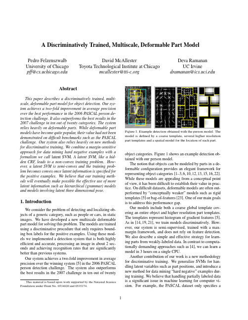
A Discriminatively Trained,Multiscale,Deformable Part ModelPedro Felzenszwalb University of Chicago pff@David McAllesterToyota Technological Institute at Chicagomcallester@Deva RamananUC Irvinedramanan@AbstractThis paper describes a discriminatively trained,multi-scale,deformable part model for object detection.Our sys-tem achieves a two-fold improvement in average precision over the best performance in the2006PASCAL person de-tection challenge.It also outperforms the best results in the 2007challenge in ten out of twenty categories.The system relies heavily on deformable parts.While deformable part models have become quite popular,their value had not been demonstrated on difficult benchmarks such as the PASCAL challenge.Our system also relies heavily on new methods for discriminative training.We combine a margin-sensitive approach for data mining hard negative examples with a formalism we call latent SVM.A latent SVM,like a hid-den CRF,leads to a non-convex training problem.How-ever,a latent SVM is semi-convex and the training prob-lem becomes convex once latent information is specified for the positive examples.We believe that our training meth-ods will eventually make possible the effective use of more latent information such as hierarchical(grammar)models and models involving latent three dimensional pose.1.IntroductionWe consider the problem of detecting and localizing ob-jects of a generic category,such as people or cars,in static images.We have developed a new multiscale deformable part model for solving this problem.The models are trained using a discriminative procedure that only requires bound-ing box labels for the positive ing these mod-els we implemented a detection system that is both highly efficient and accurate,processing an image in about2sec-onds and achieving recognition rates that are significantly better than previous systems.Our system achieves a two-fold improvement in average precision over the winning system[5]in the2006PASCAL person detection challenge.The system also outperforms the best results in the2007challenge in ten out of twenty This material is based upon work supported by the National Science Foundation under Grant No.0534820and0535174.Figure1.Example detection obtained with the person model.The model is defined by a coarse template,several higher resolution part templates and a spatial model for the location of each part. object categories.Figure1shows an example detection ob-tained with our person model.The notion that objects can be modeled by parts in a de-formable configuration provides an elegant framework for representing object categories[1–3,6,10,12,13,15,16,22]. While these models are appealing from a conceptual point of view,it has been difficult to establish their value in prac-tice.On difficult datasets,deformable models are often out-performed by“conceptually weaker”models such as rigid templates[5]or bag-of-features[23].One of our main goals is to address this performance gap.Our models include both a coarse global template cov-ering an entire object and higher resolution part templates. The templates represent histogram of gradient features[5]. As in[14,19,21],we train models discriminatively.How-ever,our system is semi-supervised,trained with a max-margin framework,and does not rely on feature detection. We also describe a simple and effective strategy for learn-ing parts from weakly-labeled data.In contrast to computa-tionally demanding approaches such as[4],we can learn a model in3hours on a single CPU.Another contribution of our work is a new methodology for discriminative training.We generalize SVMs for han-dling latent variables such as part positions,and introduce a new method for data mining“hard negative”examples dur-ing training.We believe that handling partially labeled data is a significant issue in machine learning for computer vi-sion.For example,the PASCAL dataset only specifies abounding box for each positive example of an object.We treat the position of each object part as a latent variable.We also treat the exact location of the object as a latent vari-able,requiring only that our classifier select a window that has large overlap with the labeled bounding box.A latent SVM,like a hidden CRF[19],leads to a non-convex training problem.However,unlike a hidden CRF, a latent SVM is semi-convex and the training problem be-comes convex once latent information is specified for thepositive training examples.This leads to a general coordi-nate descent algorithm for latent SVMs.System Overview Our system uses a scanning window approach.A model for an object consists of a global“root”filter and several part models.Each part model specifies a spatial model and a partfilter.The spatial model defines a set of allowed placements for a part relative to a detection window,and a deformation cost for each placement.The score of a detection window is the score of the root filter on the window plus the sum over parts,of the maxi-mum over placements of that part,of the partfilter score on the resulting subwindow minus the deformation cost.This is similar to classical part-based models[10,13].Both root and partfilters are scored by computing the dot product be-tween a set of weights and histogram of gradient(HOG) features within a window.The rootfilter is equivalent to a Dalal-Triggs model[5].The features for the partfilters are computed at twice the spatial resolution of the rootfilter. Our model is defined at afixed scale,and we detect objects by searching over an image pyramid.In training we are given a set of images annotated with bounding boxes around each instance of an object.We re-duce the detection problem to a binary classification prob-lem.Each example x is scored by a function of the form, fβ(x)=max zβ·Φ(x,z).Hereβis a vector of model pa-rameters and z are latent values(e.g.the part placements). To learn a model we define a generalization of SVMs that we call latent variable SVM(LSVM).An important prop-erty of LSVMs is that the training problem becomes convex if wefix the latent values for positive examples.This can be used in a coordinate descent algorithm.In practice we iteratively apply classical SVM training to triples( x1,z1,y1 ,..., x n,z n,y n )where z i is selected to be the best scoring latent label for x i under the model learned in the previous iteration.An initial rootfilter is generated from the bounding boxes in the PASCAL dataset. The parts are initialized from this rootfilter.2.ModelThe underlying building blocks for our models are the Histogram of Oriented Gradient(HOG)features from[5]. We represent HOG features at two different scales.Coarse features are captured by a rigid template covering anentireImage pyramidFigure2.The HOG feature pyramid and an object hypothesis de-fined in terms of a placement of the rootfilter(near the top of the pyramid)and the partfilters(near the bottom of the pyramid). detection window.Finer scale features are captured by part templates that can be moved with respect to the detection window.The spatial model for the part locations is equiv-alent to a star graph or1-fan[3]where the coarse template serves as a reference position.2.1.HOG RepresentationWe follow the construction in[5]to define a dense repre-sentation of an image at a particular resolution.The image isfirst divided into8x8non-overlapping pixel regions,or cells.For each cell we accumulate a1D histogram of gra-dient orientations over pixels in that cell.These histograms capture local shape properties but are also somewhat invari-ant to small deformations.The gradient at each pixel is discretized into one of nine orientation bins,and each pixel“votes”for the orientation of its gradient,with a strength that depends on the gradient magnitude.For color images,we compute the gradient of each color channel and pick the channel with highest gradi-ent magnitude at each pixel.Finally,the histogram of each cell is normalized with respect to the gradient energy in a neighborhood around it.We look at the four2×2blocks of cells that contain a particular cell and normalize the his-togram of the given cell with respect to the total energy in each of these blocks.This leads to a vector of length9×4 representing the local gradient information inside a cell.We define a HOG feature pyramid by computing HOG features of each level of a standard image pyramid(see Fig-ure2).Features at the top of this pyramid capture coarse gradients histogrammed over fairly large areas of the input image while features at the bottom of the pyramid capture finer gradients histogrammed over small areas.2.2.FiltersFilters are rectangular templates specifying weights for subwindows of a HOG pyramid.A w by hfilter F is a vector with w×h×9×4weights.The score of afilter is defined by taking the dot product of the weight vector and the features in a w×h subwindow of a HOG pyramid.The system in[5]uses a singlefilter to define an object model.That system detects objects from a particular class by scoring every w×h subwindow of a HOG pyramid and thresholding the scores.Let H be a HOG pyramid and p=(x,y,l)be a cell in the l-th level of the pyramid.Letφ(H,p,w,h)denote the vector obtained by concatenating the HOG features in the w×h subwindow of H with top-left corner at p.The score of F on this detection window is F·φ(H,p,w,h).Below we useφ(H,p)to denoteφ(H,p,w,h)when the dimensions are clear from context.2.3.Deformable PartsHere we consider models defined by a coarse rootfilter that covers the entire object and higher resolution partfilters covering smaller parts of the object.Figure2illustrates a placement of such a model in a HOG pyramid.The rootfil-ter location defines the detection window(the pixels inside the cells covered by thefilter).The partfilters are placed several levels down in the pyramid,so the HOG cells at that level have half the size of cells in the rootfilter level.We have found that using higher resolution features for defining partfilters is essential for obtaining high recogni-tion performance.With this approach the partfilters repre-sentfiner resolution edges that are localized to greater ac-curacy when compared to the edges represented in the root filter.For example,consider building a model for a face. The rootfilter could capture coarse resolution edges such as the face boundary while the partfilters could capture details such as eyes,nose and mouth.The model for an object with n parts is formally defined by a rootfilter F0and a set of part models(P1,...,P n) where P i=(F i,v i,s i,a i,b i).Here F i is afilter for the i-th part,v i is a two-dimensional vector specifying the center for a box of possible positions for part i relative to the root po-sition,s i gives the size of this box,while a i and b i are two-dimensional vectors specifying coefficients of a quadratic function measuring a score for each possible placement of the i-th part.Figure1illustrates a person model.A placement of a model in a HOG pyramid is given by z=(p0,...,p n),where p i=(x i,y i,l i)is the location of the rootfilter when i=0and the location of the i-th part when i>0.We assume the level of each part is such that a HOG cell at that level has half the size of a HOG cell at the root level.The score of a placement is given by the scores of eachfilter(the data term)plus a score of the placement of each part relative to the root(the spatial term), ni=0F i·φ(H,p i)+ni=1a i·(˜x i,˜y i)+b i·(˜x2i,˜y2i),(1)where(˜x i,˜y i)=((x i,y i)−2(x,y)+v i)/s i gives the lo-cation of the i-th part relative to the root location.Both˜x i and˜y i should be between−1and1.There is a large(exponential)number of placements for a model in a HOG pyramid.We use dynamic programming and distance transforms techniques[9,10]to compute the best location for the parts of a model as a function of the root location.This takes O(nk)time,where n is the number of parts in the model and k is the number of cells in the HOG pyramid.To detect objects in an image we score root locations according to the best possible placement of the parts and threshold this score.The score of a placement z can be expressed in terms of the dot product,β·ψ(H,z),between a vector of model parametersβand a vectorψ(H,z),β=(F0,...,F n,a1,b1...,a n,b n).ψ(H,z)=(φ(H,p0),φ(H,p1),...φ(H,p n),˜x1,˜y1,˜x21,˜y21,...,˜x n,˜y n,˜x2n,˜y2n,). We use this representation for learning the model parame-ters as it makes a connection between our deformable mod-els and linear classifiers.On interesting aspect of the spatial models defined here is that we allow for the coefficients(a i,b i)to be negative. This is more general than the quadratic“spring”cost that has been used in previous work.3.LearningThe PASCAL training data consists of a large set of im-ages with bounding boxes around each instance of an ob-ject.We reduce the problem of learning a deformable part model with this data to a binary classification problem.Let D=( x1,y1 ,..., x n,y n )be a set of labeled exam-ples where y i∈{−1,1}and x i specifies a HOG pyramid, H(x i),together with a range,Z(x i),of valid placements for the root and partfilters.We construct a positive exam-ple from each bounding box in the training set.For these ex-amples we define Z(x i)so the rootfilter must be placed to overlap the bounding box by at least50%.Negative exam-ples come from images that do not contain the target object. Each placement of the rootfilter in such an image yields a negative training example.Note that for the positive examples we treat both the part locations and the exact location of the rootfilter as latent variables.We have found that allowing uncertainty in the root location during training significantly improves the per-formance of the system(see Section4).tent SVMsA latent SVM is defined as follows.We assume that each example x is scored by a function of the form,fβ(x)=maxz∈Z(x)β·Φ(x,z),(2)whereβis a vector of model parameters and z is a set of latent values.For our deformable models we define Φ(x,z)=ψ(H(x),z)so thatβ·Φ(x,z)is the score of placing the model according to z.In analogy to classical SVMs we would like to trainβfrom labeled examples D=( x1,y1 ,..., x n,y n )by optimizing the following objective function,β∗(D)=argminβλ||β||2+ni=1max(0,1−y i fβ(x i)).(3)By restricting the latent domains Z(x i)to a single choice, fβbecomes linear inβ,and we obtain linear SVMs as a special case of latent tent SVMs are instances of the general class of energy-based models[18].3.2.Semi-ConvexityNote that fβ(x)as defined in(2)is a maximum of func-tions each of which is linear inβ.Hence fβ(x)is convex inβ.This implies that the hinge loss max(0,1−y i fβ(x i)) is convex inβwhen y i=−1.That is,the loss function is convex inβfor negative examples.We call this property of the loss function semi-convexity.Consider an LSVM where the latent domains Z(x i)for the positive examples are restricted to a single choice.The loss due to each positive example is now bined with the semi-convexity property,(3)becomes convex inβ.If the labels for the positive examples are notfixed we can compute a local optimum of(3)using a coordinate de-scent algorithm:1.Holdingβfixed,optimize the latent values for the pos-itive examples z i=argmax z∈Z(xi )β·Φ(x,z).2.Holding{z i}fixed for positive examples,optimizeβby solving the convex problem defined above.It can be shown that both steps always improve or maintain the value of the objective function in(3).If both steps main-tain the value we have a strong local optimum of(3),in the sense that Step1searches over an exponentially large space of latent labels for positive examples while Step2simulta-neously searches over weight vectors and an exponentially large space of latent labels for negative examples.3.3.Data Mining Hard NegativesIn object detection the vast majority of training exam-ples are negative.This makes it infeasible to consider all negative examples at a time.Instead,it is common to con-struct training data consisting of the positive instances and “hard negative”instances,where the hard negatives are data mined from the very large set of possible negative examples.Here we describe a general method for data mining ex-amples for SVMs and latent SVMs.The method iteratively solves subproblems using only hard instances.The innova-tion of our approach is a theoretical guarantee that it leads to the exact solution of the training problem defined using the complete training set.Our results require the use of a margin-sensitive definition of hard examples.The results described here apply both to classical SVMs and to the problem defined by Step2of the coordinate de-scent algorithm for latent SVMs.We omit the proofs of the theorems due to lack of space.These results are related to working set methods[17].We define the hard instances of D relative toβas,M(β,D)={ x,y ∈D|yfβ(x)≤1}.(4)That is,M(β,D)are training examples that are incorrectly classified or near the margin of the classifier defined byβ. We can show thatβ∗(D)only depends on hard instances. Theorem1.Let C be a subset of the examples in D.If M(β∗(D),D)⊆C thenβ∗(C)=β∗(D).This implies that in principle we could train a model us-ing a small set of examples.However,this set is defined in terms of the optimal modelβ∗(D).Given afixedβwe can use M(β,D)to approximate M(β∗(D),D).This suggests an iterative algorithm where we repeatedly compute a model from the hard instances de-fined by the model from the last iteration.This is further justified by the followingfixed-point theorem.Theorem2.Ifβ∗(M(β,D))=βthenβ=β∗(D).Let C be an initial“cache”of examples.In practice we can take the positive examples together with random nega-tive examples.Consider the following iterative algorithm: 1.Letβ:=β∗(C).2.Shrink C by letting C:=M(β,C).3.Grow C by adding examples from M(β,D)up to amemory limit L.Theorem3.If|C|<L after each iteration of Step2,the algorithm will converge toβ=β∗(D)infinite time.3.4.Implementation detailsMany of the ideas discussed here are only approximately implemented in our current system.In practice,when train-ing a latent SVM we iteratively apply classical SVM train-ing to triples x1,z1,y1 ,..., x n,z n,y n where z i is se-lected to be the best scoring latent label for x i under themodel trained in the previous iteration.Each of these triples leads to an example Φ(x i,z i),y i for training a linear clas-sifier.This allows us to use a highly optimized SVM pack-age(SVMLight[17]).On a single CPU,the entire training process takes3to4hours per object class in the PASCAL datasets,including initialization of the parts.Root Filter Initialization:For each category,we auto-matically select the dimensions of the rootfilter by looking at statistics of the bounding boxes in the training data.1We train an initial rootfilter F0using an SVM with no latent variables.The positive examples are constructed from the unoccluded training examples(as labeled in the PASCAL data).These examples are anisotropically scaled to the size and aspect ratio of thefilter.We use random subwindows from negative images to generate negative examples.Root Filter Update:Given the initial rootfilter trained as above,for each bounding box in the training set wefind the best-scoring placement for thefilter that significantly overlaps with the bounding box.We do this using the orig-inal,un-scaled images.We retrain F0with the new positive set and the original random negative set,iterating twice.Part Initialization:We employ a simple heuristic to ini-tialize six parts from the rootfilter trained above.First,we select an area a such that6a equals80%of the area of the rootfilter.We greedily select the rectangular region of area a from the rootfilter that has the most positive energy.We zero out the weights in this region and repeat until six parts are selected.The partfilters are initialized from the rootfil-ter values in the subwindow selected for the part,butfilled in to handle the higher spatial resolution of the part.The initial deformation costs measure the squared norm of a dis-placement with a i=(0,0)and b i=−(1,1).Model Update:To update a model we construct new training data triples.For each positive bounding box in the training data,we apply the existing detector at all positions and scales with at least a50%overlap with the given bound-ing box.Among these we select the highest scoring place-ment as the positive example corresponding to this training bounding box(Figure3).Negative examples are selected byfinding high scoring detections in images not containing the target object.We add negative examples to a cache un-til we encounterfile size limits.A new model is trained by running SVMLight on the positive and negative examples, each labeled with part placements.We update the model10 times using the cache scheme described above.In each it-eration we keep the hard instances from the previous cache and add as many new hard instances as possible within the memory limit.Toward thefinal iterations,we are able to include all hard instances,M(β,D),in the cache.1We picked a simple heuristic by cross-validating over5object classes. We set the model aspect to be the most common(mode)aspect in the data. We set the model size to be the largest size not larger than80%of thedata.Figure3.The image on the left shows the optimization of the la-tent variables for a positive example.The dotted box is the bound-ing box label provided in the PASCAL training set.The large solid box shows the placement of the detection window while the smaller solid boxes show the placements of the parts.The image on the right shows a hard-negative example.4.ResultsWe evaluated our system using the PASCAL VOC2006 and2007comp3challenge datasets and protocol.We refer to[7,8]for details,but emphasize that both challenges are widely acknowledged as difficult testbeds for object detec-tion.Each dataset contains several thousand images of real-world scenes.The datasets specify ground-truth bounding boxes for several object classes,and a detection is consid-ered correct when it overlaps more than50%with a ground-truth bounding box.One scores a system by the average precision(AP)of its precision-recall curve across a testset.Recent work in pedestrian detection has tended to report detection rates versus false positives per window,measured with cropped positive examples and negative images with-out objects of interest.These scores are tied to the reso-lution of the scanning window search and ignore effects of non-maximum suppression,making it difficult to compare different systems.We believe the PASCAL scoring method gives a more reliable measure of performance.The2007challenge has20object categories.We entered a preliminary version of our system in the official competi-tion,and obtained the best score in6categories.Our current system obtains the highest score in10categories,and the second highest score in6categories.Table1summarizes the results.Our system performs well on rigid objects such as cars and sofas as well as highly deformable objects such as per-sons and horses.We also note that our system is successful when given a large or small amount of training data.There are roughly4700positive training examples in the person category but only250in the sofa category.Figure4shows some of the models we learned.Figure5shows some ex-ample detections.We evaluated different components of our system on the longer-established2006person dataset.The top AP scoreaero bike bird boat bottle bus car cat chair cow table dog horse mbike person plant sheep sofa train tvOur rank 31211224111422112141Our score .180.411.092.098.249.349.396.110.155.165.110.062.301.337.267.140.141.156.206.336Darmstadt .301INRIA Normal .092.246.012.002.068.197.265.018.097.039.017.016.225.153.121.093.002.102.157.242INRIA Plus.136.287.041.025.077.279.294.132.106.127.067.071.335.249.092.072.011.092.242.275IRISA .281.318.026.097.119.289.227.221.175.253MPI Center .060.110.028.031.000.164.172.208.002.044.049.141.198.170.091.004.091.034.237.051MPI ESSOL.152.157.098.016.001.186.120.240.007.061.098.162.034.208.117.002.046.147.110.054Oxford .262.409.393.432.375.334TKK .186.078.043.072.002.116.184.050.028.100.086.126.186.135.061.019.036.058.067.090Table 1.PASCAL VOC 2007results.Average precision scores of our system and other systems that entered the competition [7].Empty boxes indicate that a method was not tested in the corresponding class.The best score in each class is shown in bold.Our current system ranks first in 10out of 20classes.A preliminary version of our system ranked first in 6classes in the official competition.BottleCarBicycleSofaFigure 4.Some models learned from the PASCAL VOC 2007dataset.We show the total energy in each orientation of the HOG cells in the root and part filters,with the part filters placed at the center of the allowable displacements.We also show the spatial model for each part,where bright values represent “cheap”placements,and dark values represent “expensive”placements.in the PASCAL competition was .16,obtained using a rigid template model of HOG features [5].The best previous re-sult of.19adds a segmentation-based verification step [20].Figure 6summarizes the performance of several models we trained.Our root-only model is equivalent to the model from [5]and it scores slightly higher at .18.Performance jumps to .24when the model is trained with a LSVM that selects a latent position and scale for each positive example.This suggests LSVMs are useful even for rigid templates because they allow for self-adjustment of the detection win-dow in the training examples.Adding deformable parts in-creases performance to .34AP —a factor of two above the best previous score.Finally,we trained a model with partsbut no root filter and obtained .29AP.This illustrates the advantage of using a multiscale representation.We also investigated the effect of the spatial model and allowable deformations on the 2006person dataset.Recall that s i is the allowable displacement of a part,measured in HOG cells.We trained a rigid model with high-resolution parts by setting s i to 0.This model outperforms the root-only system by .27to .24.If we increase the amount of allowable displacements without using a deformation cost,we start to approach a bag-of-features.Performance peaks at s i =1,suggesting it is useful to constrain the part dis-placements.The optimal strategy allows for larger displace-ments while using an explicit deformation cost.The follow-Figure 5.Some results from the PASCAL 2007dataset.Each row shows detections using a model for a specific class (Person,Bottle,Car,Sofa,Bicycle,Horse).The first three columns show correct detections while the last column shows false positives.Our system is able to detect objects over a wide range of scales (such as the cars)and poses (such as the horses).The system can also detect partially occluded objects such as a person behind a bush.Note how the false detections are often quite reasonable,for example detecting a bus with the car model,a bicycle sign with the bicycle model,or a dog with the horse model.In general the part filters represent meaningful object parts that are well localized in each detection such as the head in the person model.Figure6.Evaluation of our system on the PASCAL VOC2006 person dataset.Root uses only a rootfilter and no latent place-ment of the detection windows on positive examples.Root+Latent uses a rootfilter with latent placement of the detection windows. Parts+Latent is a part-based system with latent detection windows but no rootfilter.Root+Parts+Latent includes both root and part filters,and latent placement of the detection windows.ing table shows AP as a function of freely allowable defor-mation in thefirst three columns.The last column gives the performance when using a quadratic deformation cost and an allowable displacement of2HOG cells.s i01232+quadratic costAP.27.33.31.31.345.DiscussionWe introduced a general framework for training SVMs with latent structure.We used it to build a recognition sys-tem based on multiscale,deformable models.Experimental results on difficult benchmark data suggests our system is the current state-of-the-art in object detection.LSVMs allow for exploration of additional latent struc-ture for recognition.One can consider deeper part hierar-chies(parts with parts),mixture models(frontal vs.side cars),and three-dimensional pose.We would like to train and detect multiple classes together using a shared vocab-ulary of parts(perhaps visual words).We also plan to use A*search[11]to efficiently search over latent parameters during detection.References[1]Y.Amit and A.Trouve.POP:Patchwork of parts models forobject recognition.IJCV,75(2):267–282,November2007.[2]M.Burl,M.Weber,and P.Perona.A probabilistic approachto object recognition using local photometry and global ge-ometry.In ECCV,pages II:628–641,1998.[3] D.Crandall,P.Felzenszwalb,and D.Huttenlocher.Spatialpriors for part-based recognition using statistical models.In CVPR,pages10–17,2005.[4] D.Crandall and D.Huttenlocher.Weakly supervised learn-ing of part-based spatial models for visual object recognition.In ECCV,pages I:16–29,2006.[5]N.Dalal and B.Triggs.Histograms of oriented gradients forhuman detection.In CVPR,pages I:886–893,2005.[6] B.Epshtein and S.Ullman.Semantic hierarchies for recog-nizing objects and parts.In CVPR,2007.[7]M.Everingham,L.Van Gool,C.K.I.Williams,J.Winn,and A.Zisserman.The PASCAL Visual Object Classes Challenge2007(VOC2007)Results./challenges/VOC/voc2007/workshop.[8]M.Everingham, A.Zisserman, C.K.I.Williams,andL.Van Gool.The PASCAL Visual Object Classes Challenge2006(VOC2006)Results./challenges/VOC/voc2006/results.pdf.[9]P.Felzenszwalb and D.Huttenlocher.Distance transformsof sampled functions.Cornell Computing and Information Science Technical Report TR2004-1963,September2004.[10]P.Felzenszwalb and D.Huttenlocher.Pictorial structures forobject recognition.IJCV,61(1),2005.[11]P.Felzenszwalb and D.McAllester.The generalized A*ar-chitecture.JAIR,29:153–190,2007.[12]R.Fergus,P.Perona,and A.Zisserman.Object class recog-nition by unsupervised scale-invariant learning.In CVPR, 2003.[13]M.Fischler and R.Elschlager.The representation andmatching of pictorial structures.IEEE Transactions on Com-puter,22(1):67–92,January1973.[14] A.Holub and P.Perona.A discriminative framework formodelling object classes.In CVPR,pages I:664–671,2005.[15]S.Ioffe and D.Forsyth.Probabilistic methods forfindingpeople.IJCV,43(1):45–68,June2001.[16]Y.Jin and S.Geman.Context and hierarchy in a probabilisticimage model.In CVPR,pages II:2145–2152,2006.[17]T.Joachims.Making large-scale svm learning practical.InB.Sch¨o lkopf,C.Burges,and A.Smola,editors,Advances inKernel Methods-Support Vector Learning.MIT Press,1999.[18]Y.LeCun,S.Chopra,R.Hadsell,R.Marc’Aurelio,andF.Huang.A tutorial on energy-based learning.InG.Bakir,T.Hofman,B.Sch¨o lkopf,A.Smola,and B.Taskar,editors, Predicting Structured Data.MIT Press,2006.[19] A.Quattoni,S.Wang,L.Morency,M.Collins,and T.Dar-rell.Hidden conditional randomfields.PAMI,29(10):1848–1852,October2007.[20] ing segmentation to verify object hypothe-ses.In CVPR,pages1–8,2007.[21] D.Ramanan and C.Sminchisescu.Training deformablemodels for localization.In CVPR,pages I:206–213,2006.[22]H.Schneiderman and T.Kanade.Object detection using thestatistics of parts.IJCV,56(3):151–177,February2004. [23]J.Zhang,M.Marszalek,zebnik,and C.Schmid.Localfeatures and kernels for classification of texture and object categories:A comprehensive study.IJCV,73(2):213–238, June2007.。
__attribute__详解及应用

__attribute__详解及应⽤之前做过App的启动优化,遇到了+load优化的问题,后来想⼀想除了initializers代替+load还有没有什么好的⽅法,然后就搜到了运⽤编译属性__attribute__优化,于是查找了很多⽂章,系统的整理了下__attribute__。
本⽂⼤部分内容来⾃引⽤的⽂章,如果想看更多更详细内容可以查看引⽤⽂章。
__attribute__ 介绍__attribute__是⼀个编译属性,⽤于向编译器描述特殊的标识、错误检查或⾼级优化。
它是GNU C特⾊之⼀,系统中有许多地⽅使⽤到。
__attribute__可以设置函数属性(Function Attribute )、变量属性(Variable Attribute )和类型属性(Type Attribute)等。
__attribute__ 格式12__attribute__ ((attribute-list))__attribute__ 常⽤的编译属性及简单应⽤format这个属性指定⼀个函数⽐如printf,scanf作为参数,这使编译器能够根据代码中提供的参数检查格式字符串。
对于追踪难以发现的错误⾮常有帮助。
format参数的使⽤如下:1format (archetype, string-index, first-to-check)第⼀参数需要传递archetype指定是哪种风格,这⾥是 NSString;string-index指定传⼊函数的第⼏个参数是格式化字符串;first-to-check指定第⼀个可变参数所在的索引.C中的使⽤⽅法12extern int my_printf (void *my_object, const char *my_format, ...) __attribute__((format(printf, 2, 3)));在Objective-C 中通过使⽤__NSString__格式达到同样的效果,就像在NSString +stringWithFormat:和NSLog()⾥使⽤字符串格式⼀样1 2 3FOUNDATION_EXPORT void NSLog(NSString *format, ...) NS_FORMAT_FUNCTION(1,2); + (instancetype)stringWithFormat:(NSString *)format, ... NS_FORMAT_FUNCTION(1,2);__attribute__((constructor))确保此函数在在main函数被调⽤之前调⽤,iOS中在+load之后main之前执⾏。
__attribute__你知多少?

__attribute__你知多少?__attribute__ 你知多少?GNU C 的⼀⼤特⾊就是__attribute__ 机制。
__attribute__ 可以设置函数属性(Function Attribute )、变量属性(Variable Attribute )和类型属性(Type Attribute )。
__attribute__ 书写特征是:__attribute__ 前后都有两个下划线,并切后⾯会紧跟⼀对原括弧,括弧⾥⾯是相应的__attribute__ 参数。
__attribute__ 语法格式为:__attribute__ ((attribute-list))其位置约束为:放于声明的尾部“ ;” 之前。
关键字__attribute__ 也可以对结构体(struct )或共⽤体(union )进⾏属性设置。
⼤致有六个参数值可以被设定,即:aligned, packed, transparent_union, unused, deprecated 和 may_alias 。
在使⽤__attribute__ 参数时,你也可以在参数的前后都加上“__” (两个下划线),例如,使⽤__aligned__⽽不是aligned ,这样,你就可以在相应的头⽂件⾥使⽤它⽽不⽤关⼼头⽂件⾥是否有重名的宏定义。
aligned (alignment)该属性设定⼀个指定⼤⼩的对齐格式(以字节为单位),例如:struct S {short b[3];} __attribute__ ((aligned (8)));typedef int int32_t __attribute__ ((aligned (8)));该声明将强制编译器确保(尽它所能)变量类型为struct S 或者int32_t 的变量在分配空间时采⽤8 字节对齐⽅式。
如上所述,你可以⼿动指定对齐的格式,同样,你也可以使⽤默认的对齐⽅式。
如果aligned 后⾯不紧跟⼀个指定的数字值,那么编译器将依据你的⽬标机器情况使⽤最⼤最有益的对齐⽅式。
cf模型加权因子解决知识冲突

cf模型加权因子解决知识冲突
要掌握C-F模型首先需要了解可信度的概念,可信度是根据经验对一个事物或现象为真的相信程度,说白了就是有多大把握相信一个事情。
由于可信度不可避免地带有较大主观性和经验性,难以把握准确性。
C-F模型便是基于可信度表示的不确定性推理的基本方法。
不确定性推理主要有两种不确定性,即关于知识的不确定性和关于证据的不确定性。
C-F模型中关于知识的不确定性的表示方法为“IF E THEN H (CF(H,E))”。
这样的式子后面的括号中都会有一个数值,这个数值叫可信度因子,它的取值范围为[-1,1]。
可信度因子又被称为静态强度,即当E所对应的证据为真时对H的影响程度。
若CF(H,E) > 0,CF(H,E)的值越大,则证据的出现越是支持H 为真;若CF(H,E) < 0,CF(H,E)的值越小,则证据的出现越是支持H 为假;若CF(H,E)=0,则证据的出现与否与H无关。
C-F模型中关于证据的不确定性的表示方法为“CF(E)”,CF(E)的值便是证据E的可信度,它的取值范围为[-1,1]。
可信度又被称为动态强度,即证据E当前的不确定性程度。
对于初始证据,若所有观察S能肯定它为真,则CF(E) = 1。
若肯定它为假,则CF(E) = -1。
若以某种程度为真,则 0 < CF(E) < 1。
若以某种程度为假,则 -1 < CF(E) < 0 。
若未获得任何相关的观察,则 CF(E) = 0。
fmclassifier 参数

主题:fmclassifier 参数目录:1. 什么是fmclassifier?2. fmclassifier 参数介绍3. fmclassifier 参数调优4. 结语---1. 什么是fmclassifier?fmclassifier是一种基于因子分解机(Factorization Machine)的分类器模型,它结合了线性模型和因子分解机模型的优点,可以有效处理高维稀疏数据,并在推荐系统、广告点击率预测、文本分类等领域取得了广泛的成功。
2. fmclassifier 参数介绍fmclassifier参数包括两部分,一部分是模型结构相关的参数,另一部分是模型训练相关的参数。
模型结构相关参数包括:- 因子分解机的隐向量维度:控制因子分解机模型的复杂度,一般取值范围为[10, 100]。
- 正则化参数:用于控制模型的复杂度,防止过拟合,一般取值范围为[0.001, 10]。
- 是否使用一阶项:控制是否使用线性模型的一阶项特征,一般情况下建议使用。
模型训练相关参数包括:- 学习率:用于更新参数的步长,一般取值范围为[0.001, 0.1]。
- 迭代次数:模型训练的迭代次数,一般取值范围为[10, 1000]。
- 批量大小:每次迭代所用的样本数,一般取值范围为[32, 1024]。
3. fmclassifier 参数调优要调优fmclassifier模型的参数,首先需要明确目标。
如果是最大化模型的预测准确率,可以使用交叉验证和网格搜索来寻找最优的参数组合。
在调优过程中,需要注意以下几点:- 隐向量维度和正则化参数通常需要进行相互调优,以达到最佳的模型复杂度和泛化能力。
- 学习率和迭代次数需要进行相互调优,确保在模型训练过程中能够快速收敛并取得良好的效果。
- 批量大小通常可以根据训练样本的规模和计算资源进行灵活调整,以达到最佳的训练速度和效果。
在调优完成后,可以使用最优的参数组合来重新训练模型,得到最终的fmclassifier模型,以用于实际的应用场景。
刘萍萍翻译

定义色的色域边界的测试目标Phil Green彩色影像集团LCP的,英国伦敦2000年12月1.简介在生产中的一个色域是颜色可以在其上复制的范围。
这个范围将取决于许多因素,其中最重要的是介质本身的物理性能和它们一起使用的着色剂。
其他因素包括介质存在的条件,半色调或采纳抖动的方法,和在渲染过程中的任何特性或限制,如固体密度或墨水限制。
在一些行业如报纸的生产,这些因素很多是有一定程度的标准化,并有可能定义一个色域将适用(有一些变化)跨越大部分产品印刷的过程。
虽然色域通常代表两个方面(如xy色度或CIELAB的a* / b *值),这可能会引起误解的原因有两个。
首先,它忽略了亮度范围的可复制(也称为动态范围),这是色域的一个重要方面;第二,通过忽略亮度尺寸可能会出现一个给定的色域里面的颜色,而事实上并非如此。
对于硬拷贝的媒体,如着色剂的组合并不按照简单的加法原则,色域在色彩空间如CIELAB空间中是一种不规则的固体。
在CIELAB中比较不同介质的色域,我们注意到一些非常大的差异,也就是说,摄影逆转材料,而中冷置新闻纸用于重现。
可能对色域最明显有用的信息是援助在原始和繁殖媒体之间的映射颜色的过程。
色域映射算法使用双方媒体的色域边界,来确定需要多少压缩,使比较大的色域适合较小的色域。
这通常需要找到与色域边界一行的交集,通过要映射的点从收敛域边界点(通常在位于轴色差)找。
在最近的一项色域映射模型研究中,来源于高品质的复制品经验发现与经验数据拟合的模型可以通过由包括线性插值从模型中的色域边界形状的'尖'(在给定色相角度最大色度)来改善。
1.1色域边界计算色域边界的许多方法被描述在[1,2,3,4,5,6]。
这些方法的主要特点由Morovic[6进行了总结]。
不同的媒体和图像的色域也已在最近文件[7,8]中进行了比较。
在着色剂空间,色域边界可以被视为一个立方体因为在顶点它有固体着色剂和他们的第二组合的面孔。
- 1、下载文档前请自行甄别文档内容的完整性,平台不提供额外的编辑、内容补充、找答案等附加服务。
- 2、"仅部分预览"的文档,不可在线预览部分如存在完整性等问题,可反馈申请退款(可完整预览的文档不适用该条件!)。
- 3、如文档侵犯您的权益,请联系客服反馈,我们会尽快为您处理(人工客服工作时间:9:00-18:30)。
Attribute and Simile Classifiers for Face VerificationNeeraj Kumar Alexander C.Berg Peter N.Belhumeur Shree K.NayarColumbia University∗AbstractWe present two novel methods for face verification.Our first method–“attribute”classifiers–uses binary classi-fiers trained to recognize the presence or absence of de-scribable aspects of visual appearance(e.g.,gender,race, and age).Our second method–“simile”classifiers–re-moves the manual labeling required for attribute classifica-tion and instead learns the similarity of faces,or regions of faces,to specific reference people.Neither method re-quires costly,often brittle,alignment between image pairs; yet,both methods produce compact visual descriptions,and work on real-world images.Furthermore,both the attribute and simile classifiers improve on the current state-of-the-art for the LFW data set,reducing the error rates compared to the current best by23.92%and26.34%,respectively,and 31.68%when combined.For further testing across pose, illumination,and expression,we introduce a new data set–termed PubFig–of real-world images of publicfigures (celebrities and politicians)acquired from the internet.This data set is both larger(60,000images)and deeper(300 images per individual)than existing data sets of its kind. Finally,we present an evaluation of human performance.1.IntroductionThere is enormous variability in the manner in which the same face presents itself to a camera:not only might the pose differ,but so might the expression and hairstyle.Mak-ing matters worse–at least for researchers in computer vi-sion–is that the illumination direction,camera type,focus, resolution,and image compression are all almost certain to differ as well.These manifold differences in images of the same person have confounded methods for automatic face recognition and verification,often limiting the reliability of automatic algorithms to the domain of more controlled set-tings with cooperative subjects[33,3,29,16,30,31,14].Recently,there has been significant work on the“La-beled Faces in the Wild”(LFW)data set[19].This data set is remarkable in its variability,exhibiting all of the differences mentioned above.Not surprisingly,LFW has proven difficult for automatic face verification methods [25,34,17,18,19].When one analyzes the failure cases for ∗{neeraj,aberg,belhumeur,nayar}@ Figure1:Attribute Classifiers:An attribute classifier can be trained to recognize the presence or absence of a describable as-pect of visual appearance.The responses for several such attribute classifiers are shown for a pair of images of Halle Berry.Note that the“flash”and“shiny skin”attributes produce very differ-ent responses,while the responses for the remaining attributes are in strong agreement despite the changes in pose,illumination,ex-pression,and image quality.We use these attributes for face verifi-cation,achieving a23.92%drop in error rates on the LFW bench-mark compared to the existing state-of-the-art.some of the existing algorithms,many mistakes are found that would seem to be avoidable:men being confused for women,young people for old,asians for caucasians,etc.On the other hand,small changes in pose,expression,or light-ing can cause two otherwise similar images of the same per-son to be mis-classified by an algorithm as different.How-ever,we show that humans do very well on the same data–given image pairs,verification of identity can be performed almost without error.In this paper,we attempt to advance the state-of-the-art for face verification in uncontrolled settings with non-cooperative subjects.To this end,we present two novel and complementary methods for face verifimon to both methods is the idea of extracting and comparing “high-level”visual features,or traits,of a face image that方法一是“属性分类器”,用二进制的训练过的分类器来识别是否有视觉外观方面的描述(例如性别、种族和年龄)第二种方法“笑脸分类器”将属性分类器需要的人工标签移除,而学习脸部的相似点或区域多方面的are insensitive to pose,illumination,expression,and other imaging conditions.These methods also have the advantage that the training data they require is easier to acquire than collecting a large gallery of images per enrolled individual (as is needed by traditional face recognition systems).Ourfirst method–based on attribute classifiers–uses binary classifiers trained to recognize the presence or ab-sence of describable aspects of visual appearance(gender, race,age,hair color,etc.).We call these visual traits“at-tributes,”following the name and method of[21].For ex-ample,Figure1shows the values of various attributes for two images of Halle Berry.Note that the“flash”and“shiny skin”attributes produce very different responses,while the responses for the remaining attributes are in strong agree-ment despite the changes in pose,illumination,and expres-sion.To date,we have built sixty-five attribute classifiers, although one could train many more.Our second method–based on simile classifiers–re-moves the manual labeling required to train attribute clas-sifiers.The simile classifiers are binary classifiers trained to recognize the similarity of faces,or regions of faces,to specific reference people.We call these visual traits“simi-les.”The idea is to automatically learn similes that distin-guish a person from the general population.An unseen face might be described as having a mouth that looks like Barack Obama’s and a nose that looks like Owen Wilson’s.Figure2 shows the responses for several such simile classifiers for a pair of images of Harrison Ford.R j denotes reference per-son j,so thefirst bar on the left displays similarity to the eyes of reference person1.Note that the responses are,for the most part,in agreement despite the changes in pose,il-lumination,and expression.To date,we have used sixty ref-erence people to build our simile classifiers,although many more could be added with little effort.Our approach for face verification does not use expen-sive computation to align pairs of faces.The relatively short (65–3000dimensional)vector of outputs from the trait clas-sifiers(attribute and simile)are computed on each face paring two faces is simply a matter of com-paring these trait vectors.Remarkably,both the attribute and simile classifiers give state-of-the-art results,reducing the previous best error rates[34]on LFW[19]by23.92% and26.34%,respectively.To our knowledge this is thefirst time visual traits have been used for face verification.As the attribute and simile classifiers offer complemen-tary information,one would expect that combining these would further lower the error rates.For instance,it is pos-sible for two people of different genders to have eyes like Salma Hayek’s and noses like Meryl Streep’s.So,while the simile classifier might confuse these,the attribute classifier would not.Our experiments seem to support this,as com-bining the attributes and similes together reduce the previ-ous best error rates by31.68%.Figure2:Simile Classifiers:We use a large number of“simile”classifiers trained to recognize the similarities of parts of faces to specific reference people.The responses for several such simile classifiers are shown for a pair of images of Harrison Ford.R j denotes reference person j,so thefirst bar on the left displays the similarity to the eyes of reference person1.Note that the re-sponses are,for the most part,in agreement despite the changes in pose,illumination,and expression.We use these similes for face verification,achieving a26.34%drop in error rates on the LFW benchmark compared to the existing state-of-the-art.For testing beyond the LFW data set,we introduce Pub-Fig–a new data set of real-world images of publicfigures (celebrities and politicians)acquired from the internet.The PubFig data set is both larger(60,000images)and deeper (on average300images per individual)than existing data sets,and allows us to present verification results broken out by pose,illumination,and expression.We summarize the contributions of the paper below: 1.Attribute Classifiers:We introduce classifiers forface verification,using65describable visual traits such as gender,age,race,hair color,etc.;the classi-fiers improve on the state-of-the-art,reducing overall error rates by23.92%on LFW.2.Simile Classifiers:We introduce classifiers for faceverification,using similarities to a set of60reference faces;the classifiers improve on the state-of-the-art, reducing overall error rates by26.34%on LFW.The simile classifiers do not require the manual labeling of training sets.3.PubFig Data set:We introduce PubFig,thelargest data set of real-world images(60,000) for face verification(and recognition),publicly available at / CAVE/databases/pubfig/.4.Human Performance Evaluation:We present anevaluation of human performance on the LFW data set.提取并比较一张人脸图像的高级视觉特征,这些特征对姿态、光线、表情和其他图像情况并不敏感对每一张脸都独立地计算相应的特征分类器中输出图像的短向量(65-3000维)2.Related WorkIt is well understood that variation in pose and expression and,to a lesser extent,lighting cause significant difficul-ties for recognizing the identity of a person[35].The Pose, Illumination,and Expression(PIE)data set and follow-on results[33]showed that sometimes alignment,especially in 3D,can overcome these difficulties[3,4,16,33,7].Unfortunately,in the setting of real-world images such as those in Huang et al.’s“Labeled Faces in the Wild”(LFW) benchmark data set[19]and similar data sets[2,10],3D alignment is difficult and has not(yet)been demonstrated. Various2D alignment strategies have been applied to LFW –aligning all faces[17]to each other,or aligning each pair of images to be considered for verification[25,11].Ap-proaches that require alignment between each image pair are computationally expensive.Our work does not require pairwise alignment.Neither does that of the previously most successful approach on LFW from Wolf et al.[34], which uses a large set of carefully designed binary patch features.However,in contrast to Wolf et al.[34],our fea-tures are designed to provide information about the identity of an individual in two ways:by recognizing describable at-tributes(attribute classifiers),and by recognizing similarity to a set of reference people(simile classifiers).Our low-level features are designed following a great deal of work in face recognition(and the larger recogni-tion community)which has identified gradient direction and local descriptors aroundfiducial features as effectivefirst steps toward dealing with illumination[6,28,22,23,10].Automatically determining the gender of a face has been an active area of research since at least1990[15,9],and includes more recent work[24]using Support Vector Ma-chines(SVMs)[8].This was later extended to the recogni-tion of ethnicity[32],pose[20],expression[1],etc.More recently,a method for automatically training classifiers for these and many other types of attributes was proposed,for the purpose of searching databases of face images[21].We follow their method for training our attribute classifiers,but improve on their feature selection process and the number of attributes considered.Gallagher and Chen[13]use esti-mates of age and gender to compute the likelihood offirst names being associated with a particular face,but to our knowledge,no previous work has used attributes as features for face verification.3.Our ApproachThefirst step of our approach is to extract“low-level”fea-tures from different regions of the face,e.g.,normalized pixel values,image gradient directions,or histograms of edge magnitudes.But as our aim is to design a face verifi-cation method that is tolerant of image changes,our second step is to use these low-level features to compute“high-level”visual features,or traits,which are insensitive to changes in pose,illumination,and expression.These vi-sual traits are simply scores of our trait classifiers(attribute or simile).To perform face verification on a pair of images, we compare the scores in both images.Our steps are for-malized below:1.Extract Low-level Features:For each face image I,we extract the output of k low-level features f i=1...k and concatenate these vectors to form a large feature vector F(I)= f1(I),···,f k(I) .pute Visual Traits:For each extracted featurevector F(I),we compute the output of n trait classi-fiers C i=1...n in order to produce a“trait vector”C(I) for the face,C(I)= C1(F(I)),···,C n(F(I)) . 3.Perform Verification:To decide if two face imagesI1and I2are of the same person,we compare their trait vectors using afinal classifier D which defines our verification function v:v(I1,I2)=D(C(I1),C(I2))(1) v(I1,I2)should be positive when the face images I1 and I2show the same person and negative otherwise.Section3.1describes the low-level features{f i}.Our trait classifiers{C i}are discussed in Section3.2(attribute classifiers)and Section3.3(simile classifiers).Thefinal classifier D is described in Section3.4.3.1.Low-level FeaturesTo extract low-level features,we follow the procedure de-scribed in[21],summarized here.Wefirst detect faces andfiducial point locations using a commercial face detec-tor[26].The faces are then rectified to a common coor-dinate system using an affine warp based on thefiducials. The low-level features are constructed by choosing a face region,a feature type to extract from this region,a normal-ization to apply to the extracted values,and an aggregation of these values.The regions were constructed by hand-labeling different parts of the rectified face images,such as the eyes,nose, mouth,etc.(To handle the larger variation of pose in our data,we slightly enlarged the regions shown in[21].)Fea-ture types include image intensities in RGB and HSV color spaces,edge magnitudes,and gradient directions.Normal-ization can be done by subtracting the mean and dividing by the standard deviation,or by just dividing by the mean,or not at all.Finally,the normalized values can be aggregated by concatenating them,collapsing them into histograms,or representing them only by their mean and variance.This produces a large number of possible low-level fea-tures,{f i},a subset of which is automatically chosen and used for each trait classifier C i,as described next.低层特征:像素值、图像梯度方向、边缘幅度直方图对每张人脸图像I,我们提取K个低层特征,并把它们联结成一个大的特征向量F(I)对每一个特征向量F(I),我们计算n个属性分类器的的输出,来产生一个属性向量C(I)最后,用一个定义了分类函数的分类器D来比较两个属性向量,以此来确定两张人脸图像是否来自同一个人基准点首先用一个商业人脸检测器来检测人脸和光基准点的位置。