stata上机实验第二讲
计量经济学stata上机教程

计量经济学stata上机教程2014计量经济学上机教程1Stata操作基础主要内容:1. Stata的特点与功能2. Stata的界面管理3. Stata的命令语法4. 数据处理5. 统计描述、制图与输出结果6. log文档与do文档7. 常用函数8. Stata的帮助系统与学习资源9. 课后练习1. Stata的特点与功能, 将统计功能与计量分析完整地结合起来。
不仅可以实现诸多统计分析方法,比如描述统计、假设检验、方差分析、主成分分析等,而且可以实现多种计量经济模型的估计和检验,包括经典单方程回归模型、方程组模型、微观数据模型(离散选择模型、计数模型、截断模型、归并模型等)、时间序列数据模型(ARMA、VAR、GARCH等)以及面板数据分析。
, 强大的数据处理功能。
, 精致的作图功能。
, 丰富的网络资源。
Stata 12有各种版本,其中尤以SE(特殊版)最为常用。
用户可以在命令栏中输入about命令查看所安装的版本信息。
2--per ml sodium hydroxide [c (NaOH) =1.000 mol/L] potassium hydrogen phthalate standard solution of quality g. ... After dilution to 1000mL. 1.1.2 0.000 35mol/L iodine solution: dissolve 20 g of potassium iodide in Cheng You (30~40) 500mL mL water bottle; 5mL iodine stock solution, and then diluted to scale and mix. This solution every other day to prepare. 1.1.3 acetate buffer (PH5.3): dissolve 87g sodium acetate (CH3COONa • 3H2O) 400mL water and 10.5mL in glacial acetic acid is dissolved in a small amount of water. volume and then mixing the two together and add water to 500mL, using regulation to PH5.3. 1.1.40.5mol/L sodium chloride: 14.5 g of sodium chloride dissolved in boiled water, and constant volume to 500mL. 1.1.5 soluble starch: pure before use should determine its value. Accurate said take amount starch (equivalent to dry state 1g) Yu 250mL high type beaker in the, added80~90mL distilled water, Yu asbestos online in constantly mixing Xia quickly heating to boiling, then with fire keep micro-boiling 3min, stamped and cooling to at room temperature, transfer to 100mL capacity bottle in the, into 40 ? water bath in the makes solution reached this temperature, and in 40 ? Shi with distilled water (40 ?) set capacity, this starch solution placed 40 ? thermostat water bath in the for determination samples with. 1.2 the instrument a) constant temperaturewater bath: (40+-0.2) 0C. B) spectrophotometer. 1.3 procedures 1.3.1 preparation of samples: weighing 50mL 10G sample不同的版本对于样本容量、变量个数、矩阵阶数等有着不同的限制,用户可以通过以下命令了解和改变这些设定:memory 显示目前存储空间query memory 查看目前实际设定的存储空间set memory 10m 设定存储空间的大小set matsize 250 设定最大矩阵阶数set maxvar 2500 设定最大变量数(最小设定为2048)help limits 显示Stata的各种极限 2. Stata的界面管理, 首次打开Stata,将会出现一个询问是否进行更新的对话框。
STATA实验课

Lab 2Four topics :Do file , Data Management, Graphics and Test after estimation1 Do file⏹s tore the commands in a file⏹s ame as Program Editor in SAS⏹s ame as m-file in MATLABthe grammar of STATA:[by varlist:] command [varlist] [=exp] [if exp] [in range] [weight][using filename] [, options] Example : create a do file and save it2 Data Management(1) Stata commands in this unitcd Change directorymemory Display a report on memory usageset memory Set the size of memoryinfile Read unformatted ASCII (text) dataclear Clear the entire dataset and everything elseinput Enter data from keyboardsave Store the dataset currently in memory on disk in Stata data formatuse Load a Stata-format dataset describe Describe contents of data in memory or on diskcount Show the number of observations list List values of variableslabel data Apply a label to a data set label variable Apply a label to a variablerename Rename a variable generate Creates a new variable keep if Keep observations if condition is metkeep Keep variables orobservationsdrop Drop variables or observationsappend Append a data file to current filesort Sort observationsmerge Merge a data file with current file(2) Example:cd d:\stata /*the folder of my Stata dataset*/ memoryset memory 200minfile str20 month RM_RF SMB HML RF using ff.txt, clearinput id str20 name math1 “Jim”952 “Lucy”803 “Li Lei”90endsave math1input id str20 name math4 “Carl”100endsave math2input id str20 name economics1 “Jim”902 “Lucy”903 “Li Lei”854 “Carl”95endsave economicsuse math1describecountlistuse math1label data “grade”label variable id “the student ID”label variable name “the student name”label variable math “the student grade of math”rename math Chineserename Chinese mathgen meanmath=90gen devmath=math-meanmathuse GPA, clearkeep if female==1keep id sat race term blackdrop race blackuse math1, cleardrop meanmath devmathappend using math2save, replaceuse math1, clearsort idsave, replaceuse economics, clearsort idsave, replaceuse math1, clearmerge id using economicssave gradeuse grade, clearlist3 Graphics(1) Benchmark[graph] twoway plot [if] [in] [, twoway_options]plot is[(] plottype varlist ..., options [)] [||](2)plottypescatterlinelfitqfitlfitci(3) example: CEO Salary and Return on Equityuse ceosal1, cleargraph twoway scatter salary roetwoway (scatter salary roe) (lfit salary roe)tw (scatter salary roe) (qfit salary roe)tw (scatter salary roe) (lfitci salary roe)tw function x^2, ra(-10 10)4 Test after estimation⏹t est coeflist⏹t est exp=exp[=...]ExampleEx 4.1use wage1, clearreg lwage educ exper tenure test educ=0.1di (0.092029-0.1)/0 .0073299 Ex 4.。
Stata操作讲义知识讲解

Stata操作讲义知识讲解S t a t a操作讲义Stata操作讲义第一讲 Stata操作入门第一节概况Stata最初由美国计算机资源中心(Computer Resource Center)研制,现在为Stata公司的产品,其最新版本为7.0版。
它操作灵活、简单、易学易用,是一个非常有特色的统计分析软件,现在已越来越受到人们的重视和欢迎,并且和SAS、SPSS一起,被称为新的三大权威统计软件。
Stata最为突出的特点是短小精悍、功能强大,其最新的7.0版整个系统只有10M左右,但已经包含了全部的统计分析、数据管理和绘图等功能,尤其是他的统计分析功能极为全面,比起1G以上大小的SAS系统也毫不逊色。
另外,由于Stata在分析时是将数据全部读入内存,在计算全部完成后才和磁盘交换数据,因此运算速度极快。
由于Stata的用户群始终定位于专业统计分析人员,因此他的操作方式也别具一格,在Windows席卷天下的时代,他一直坚持使用命令行/程序操作方式,拒不推出菜单操作系统。
但是,Stata的命令语句极为简洁明快,而且在统计分析命令的设置上又非常有条理,它将相同类型的统计模型均归在同一个命令族下,而不同命令族又可以使用相同功能的选项,这使得用户学习时极易上手。
更为令人叹服的是,Stata语句在简洁的同时又拥有着极高的灵活性,用户可以充分发挥自己的聪明才智,熟练应用各种技巧,真正做到随心所欲。
除了操作方式简洁外,Stata的用户接口在其他方面也做得非常简洁,数据格式简单,分析结果输出简洁明快,易于阅读,这一切都使得Stata成为非常适合于进行统计教学的统计软件。
Stata的另一个特点是他的许多高级统计模块均是编程人员用其宏语言写成的程序文件(ADO文件),这些文件可以自行修改、添加和下载。
用户可随时到Stata网站寻找并下载最新的升级文件。
事实上,Stata的这一特点使得他始终处于统计分析方法发展的最前沿,用户几乎总是能很快找到最新统计算法的Stata程序版本,而这也使得Stata 自身成了几大统计软件中升级最多、最频繁的一个。
stata入门操作
-1-
任务:按学号录入五个学生的经济学成绩
id
economy
1
40
2
80
3
90
4
70
5Hale Waihona Puke 53操作:在 command 窗口中键入(注:前面的点号不必健入,每完成一行按回车键,黑体为命令,
斜体为变量名或文件名):
• clear
• input id name
• 1 40
• 2 80
• 3 90
• use economy,clear • sum economy • sum • sum economy in 1/2 • sum economy in 1/4 if economy>60
补充: Format 用来控制数据输出的格式
任务 2:生成新的数据 x, (x=1,2,…1000); y=x+100. • clear • set obs 1000 • gen x=_n • gen y=x+100
• 4 70
• 5 53
• end
• save economy
• save economy,replace
• exit,clear 其中后两命令先保存数据,文件名为 economy,然后清除内存中的数据并退出 STATA. 如果重复执行 save economy 回出现错误提示”file economy have already exist”,意味着
pwd
显示当前路径
pwd
dir
列示当前路径文件夹中的所有文件 dir
mkdir
在当前路径下创建一个新的文件夹 mkdir d:/mydata
cd
将 cd 后面的路径设定为当前路径 cd “d:/mydata”
计量2之上机教程2

test (lnox=10*stratio)(ldist=stratio) lincom rooms+ldist+stratio
/*检验 H 0 : 3 4 5 0 ,“lincom”用于检验参 数的线性组合,此时不能用“test”;线性组合=0,可省 略“=0”。*/
//用约束最小二乘估计进行检验 regress lprice lnox ldist rooms stratio scalar ee0=e(rss) //估计无约束模型 //计算无约束模型的残差平方和 //估计约束模型
stdf /*实际预测值(预测误差)的标准误
ˆi yi ) xi s 1 xi X X xi */ stdfi var( y
1
估计后检验 test e. g. test x1 test x1 x2 x3 //检验 x1 对应的系数的显著性 //检验 x1 x2 x3 对应系数的联合显著性 //检验 x1 x2 对应系数 2 3 //检验 2 2 //检验 2 2 //系数线性组合的点估计、标准误、检验与推断 //线性假设检验
ˆ ,默认值 //线性预测值,即拟合值 X
//残差
e X s 1 x X X 1 x */ stdri var i i i
stdp /*条件期望预测值(预测误差)的标准误
x ˆ x X s x X X 1 x */ stdpi var i i i i
use /data/imeus/hprice2a
regress lprice regress estat ic regress,beta ereturn list predict lpricehat, xb resid lprice lnox lnox ldist rooms ldist stratio, noconstant rooms stratio
实验二

实验(实训)报告项目名称多元回归模型的矩阵计算所属课程名称应用回归分析项目类型验证性实验实验(实训)日期11年10月22 日班级09统计1学号姓名指导教师浙江财经学院教务处制实验二报告多元回归模型的矩阵计算(验证性实验)实验类型:验证性实验实验目的:使学生学会用stata 软件掌握多元回归模型的相关矩阵的计算。
实验内容:多元回归模型的矩阵计算 实验要求:运用Stata 计算多元回归的矩阵计算,按具体的题目要求完成实验报告。
并及时上传到给定的FTP !实验题目: [abstracted from 《Applied Linear Regression Models 》 (FourthEdition) chapter6 Problems 6.27]In a small-scale regression study ,the following data obtained:Using matrix methods , obtaina. βˆ b. e c. P, M d. SSR, SSEe. )(ˆ),ˆ(ˆe ar V ar Vβ f. 30,10ˆ20100==x x when yg. 30,10)ˆ(ˆ20100==x x when y ar Vh. R 2, F实验题目分析报告:a. egen one=fill(1,1). browse. mkmat y,mat(y). mkmat one x1 x2 ,mat(x). mat b=inv(x'*x)*x'*y. mat list bb[3,1]yone 33.932103x1 2.7847614x2 -.26441893b. mat m=I(6)-x*inv(x'*x)*x'. mat e=m*y. mat list ee[6,1]yr1 -2.6996084r2 -1.2299728r3 -1.6373532r4 -1.32986r5 -.08999801r6 6.9867923c. mat p=x*inv(x'*x)*x'. mat list psymmetric p[6,6]r1 r2 r3 r4 r5 r6r1 .23143293r2 .25167585 .31240459r3 .21178735 .09437844 .70442026r4 .14886839 .26627729 -.31917435 .61425632r5 -.05475543 -.14787283 .10446672 .14143492 .94039955r6 .21099091 .22313666 .20412159 .14833743 .01632707 .19708635. mat m=I(6)-p. mat list msymmetric m[6,6]r1 r2 r3 r4 r5 r6 r1 .76856707r2 -.25167585 .68759541 r3 -.21178735 -.09437844 .29557974r4 -.14886839 -.26627729 .31917435 .38574368 r5 .05475543 .14787283 -.10446672 -.14143492 .05960045 r6 -.21099091 -.22313666 -.20412159 -.14833743 -.01632707 .80291365 d. mat i=J(6,1,1). mat m0=I(6)-i*inv(i'*i)*i' . mat ssr=e'*e . mat yhat=p*y. mat sse=yhat'*m0*yhat . mat sst=y'*m0*y . mat list ssesymmetric sse[1,1] yy 3009.9265 . mat list ssrsymmetric ssr[1,1] yy 62.073538 . mat list sstsymmetric sst[1,1] yy 3072 e=2ˆδ62.073538/3=20.6912)ˆ(ˆβar V=20.6912* one x1 x2 one 34.578557 x1 -1.6508927 .08030796 x2 -.65704022 .03112763 .01268501 =onex1 x2one 715.47114 x1 -34.158917 1.6616664 x2 -13.594937 .64406737 .26246775)(ˆe ar V= r1 r2 r3 r4 r5 r6 r1 15.902559 r2 -5.2074701 14.22716 r3 -4.38213 -1.9528013 6.1158935 r4 -3.0802625 -0 5.5095913 6.6040938 7.9814916 r5 1.1329543 3.0596634 -2.1615395 -2.9264554 1.2332036 r6 -4.3656507 -4.6169606 -4.2235164 -3.0692763 -.33782638 16.61323f12ˆ33.932 2.7850.264i i i yx x =+- 时当30,102010==x x ,y0=53.862g)ˆ(ˆ0y ar V=79.653hR2=sse/sst =0.9798F=-0.758。
STATA入门PPT课件

一、数据录入、打开与保存
1.数据录入与读取
直接录入数据 input命令 读入ASCII格式原始数据——使用insheet、 infile、infix等命令 使用Stat/Transfer软件
一、数据录入、打开与保存
2. STATA数据打开 双击直接打开
Do文件中使用use命令
一、数据录入、打开与保存
[STATA演示]
三、变量类型与简单描述统计方法
7. 离散与连续变量
通常,离散变量包括了定类变量和定序变量,统计 描述可参照之;而连续变量包括了定距变量和定比 变量,统计描述同样可参照之。 值得注意的是,在社会科学研究中,定距变量和定 比变量很少单独区分。
四、练习与作业
【1】请在2014年卫计委流动人口动态监测调查数据 之“社会融合与心理健康问卷”部分识别各变量 设置的层次。
二、基本的STATA数据处理命令
6.生成虚拟(哑)变量的命令 –tab region, generate(region) 7.帮助命令
–help command
三、变量类型与简单描述统计方法
1. 变量类型
区分标准之一:离散变量与连续变量
区分标准之二:定比变量、定距变量、 定序变量与定类变量
三、变量类型与简单描述统计方法
第二讲:STATA入门
1.统计软件:STATA14.0
2.数据准备:① 2014年卫计委流动人口动态监测调 查数据之“社会融合与心理健康问卷”部分;②农 民工随迁子女城市融入课题组的“外出务工调查数 据”。
1. 数据录入、打开与保存 2. 基本的STATA数据处理命令 3. 变量类型与简单描述统计方法 4. 练习与作业
4.删除变量或观察值命令 – drop命令 – drop in 1/10 or (-10/-1) – keep命令 – keep var1 var2… – keep if
stata上机实验操作
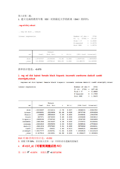
第六章第二题:1. 建立完成的教育年数(ED )对到最近大学的距离(Dist )的回归:. reg ed dist, robust斜率估计值是:-0.0732. reg ed dist bytest female black hispanic incomehi ownhome dadcoll cue80 stwmfg80,robustDist 对ED 的效应估计是:-0.0323. 系数下降50%,存在很大差异,(1)中回归存在遗漏变量偏差4. di e(r2_a)(可看到调整后的R2)第一问中=0.0074 调整的2R =0.00718796_cons 13.95586 .0378112 369.09 0.000 13.88172 14.02999dist -.0733727 .0134334 -5.46 0.000 -.0997101 -.0470353ed Coef. Std. Err. t P>|t| [95% Conf. Interval]RobustRoot MSE = 1.8074R-squared = 0.0074Prob > F = 0.0000F( 1, 3794) = 29.83Linear regression Number of obs = 3796. reg ed dist , robust2R第二问中=0.2788 2R = 0.27693235可以得到第二问中的拟合效果要优于第一问。
第二问中相似的原因:因为n 很大。
5. Dadcoll 父亲有没有念过大学:系数为正(0.6961324)衡量父亲念过大学的学生接受的教育年数平均比其父亲没有年过大学的学生多。
-.0517777 1)原因:这些参数在一定程度上构成了上大学的机会成本。
2)它们的系数估计值的符号应该如此。
当Stwmfg80增加时,放弃的工资增加,所以大学入学率降低了;因而Stwmfg80的系数对应为负。
- 1、下载文档前请自行甄别文档内容的完整性,平台不提供额外的编辑、内容补充、找答案等附加服务。
- 2、"仅部分预览"的文档,不可在线预览部分如存在完整性等问题,可反馈申请退款(可完整预览的文档不适用该条件!)。
- 3、如文档侵犯您的权益,请联系客服反馈,我们会尽快为您处理(人工客服工作时间:9:00-18:30)。
指数 交乘项 虽然对函数形式的选择有检验方法,但最好 还是从“经济意义”角度确定。
例题
例一:利用wage2的数据检验明瑟(mincer)工
资方程的简单形式: Ln(wage)=b0+b1*educ+b2*exper +b3*exper^2+ u
例二:利用phillips的数据拟合预期增强的菲
length, c(1-3) (本题没有什么经济意义,只是让大家熟悉这种方法)
矩阵运算
1。手动建立矩阵命令:matrix Matrix input 矩阵变量名=(矩阵) 同一行元素用,分隔
不同行元素用\分割
建立矩阵 :
3 5 2
6 8 11 7 18 16
显示矩阵变量
4。标准化系数
reg price mpg weight foreign, beta 5。部分数据回归
reg price mpg weight length foreign in 1/30
(为什么foreign被drop掉?)
reg price mpg weight length if foreign==0
mkmat 变量名表,mat(矩阵名)
练习:sysuse auto
reg price mpg weight foreign
要求:利用矩阵运算手动计算出参数
gen cons = 1 mkmat price, mat(y) mkmat mpg weight foreign cons, mat(X) mat b = inv(X'*X)*X'*y mat list b mat list y mat list X
通过上课的学习我们得到:
1 ˆ β ( X ' X) X ' y
习惯上我们用
/* 被解释变量的拟合值*/ e = y - y_hat = y - Xb /* 残差 */
y_hat = X*b
建立回归方程
打开系统文件auto,建立如下方程:
sysuse auto,clear regress price mpg weight foreign
lvr2plot
lvr2plot, mlabel(make)
我们可以利用矩阵运算的方法将回归结果展
现的所有统计量都手动计算出来。 大家有兴趣回去做一遍,可以加深你对这些 知识的理解。
逐步回归法
逐步回归法分为逐步剔除和逐步加入。 逐步剔除又分为逐步剔除(Backward selection)和逐步分层剔除
(Backward hierarchical selection) 1。逐步剔除 stepwise, pr(显著性水平): 回归方程 例如:对auto数据 Stepwise,pr(0.05):reg price mpg rep78 headroom trunk weight length turn displacement gear_ratio foreign
2。逐个分层加入 Stepwise,pe(0.05) hier:reg price mpg rep78 headroom
trunk weight length turn displacement gear_ratio foreign
残差点的图形表示
rvfplot:残差拟合值图 可以加参数yline(0) 将e 与ˆy 画在一起 rvpplot x1:残差预测值图 将e 与x1 画在一起 avplot avplots lvr2plot
离群样本点与杠杆样本点
离群样本点:残差值较大的样本点
杠杆样本点:与样本整体(X'X)很不相同的少 数样本点 离群样本点: reg price mpg weight foreign predict e,res List make price e
杠杆样本点:
reg price mpg weight foreign predict lev, leverage
例三:生产函数production
use production,clear reg lny lnl lnk
test lnl lnk test (lnl=0.8) (lnk=0.2) test lnk+lnl=1
非线性检验:testnl
例一
. sysuse auto gen weight2 = weight^2 reg price mpg trunk length weight weightsq foreign testnl _b[mpg] = 1/_b[weight] testnl (_b[mpg] = 1/_b[weight]) (_b[trunk] = 1/_b[length])
Stata上机实验
作业解答
作业1答案
作业2答案
添加标签
1。为整个数据添加标签:例如,将数据命名
为“工资表”。 菜单:Data->Labels->Label dataset 命令:label data “工资表“ 2。为变量增加标签,例如,给变量wage增 加标签“年工资总额” 菜单:Data->Labels->Label variables 命令 label variable wage “年工资总额"
2。逐个分层剔除 Stepwise,pr(0.05) hier:reg price mpg rep78 headroom trunk weight
length turn displacement gear_ratio foreign 去掉foreign 重新做一遍
逐步加入又分为逐步加入(Forward selection)和逐步分层加
例二: use wage2, clear reg lnwage educ tenure exper expersq 1。教育(educ)和工作时间(tenure)对工资的
影响相同。 test educ=tenure 2。工龄(exper)对工资没有影响 test exper 或者 test exper =0 3。检验 educ和 tenure的联合显著性 test educ tenure 或者 test (educ=0) (tenure=0)
2。残差的获得
predict e , residuals 或者 predict e, res
回归的假设检验
Test命令
例一 sysuse auto, clear reg price mpg weight length
1。检验参数的联合显著性
2。分别检验各参数的显著性
3。三个参数对被解释变量的影响相同
mat dir 显示矩阵内容
Mat list 矩阵变量
常用矩阵运算: C=A+B A-B A*B Kronecker乘积 :C=A#B
常用矩阵函数: trace(m1) m1的迹 Diag(v1) 向量的对角矩阵 inv(m1) m1的逆矩阵
2。还可以将变量转换为矩阵
在的异方差或自相关问题不敏感,基于稳健 标准差计算的稳健t统计量仍然渐进分布t分布。 因此,在Stata中利用robust选项可以得到异 方差稳健估计量。
约束回归
定义约束条件
constraint define n 条件 约束回归语句
Cnsreg 被解释变量 解释变量, constraints(条
Regress命令详解:
regress depvar [indepvars] [if] [in] [weight] [,
optiห้องสมุดไป่ตู้ns]
1。要求方程省略常数项(自己设置常数项)
reg price mpg weight foreign, nocons(hascons) 2。稳健性估计(一般用于大样本OLS) reg price mpg weight foreign, vce(robust) 或者:reg price mpg weight foreign, r 3。设置置信区间(默认95%) reg price mpg weight foreign, level(99)
回归结果解读
系数/标准误差= t值 P值 系数=0的概率为 p值 在5%的水准上显著不为0 否则和0的差异不显著 95%下限=估计值-t值*标准误差 95%下限=估计值+t值*标准误差 置信区间: 系数在95%的概率下会落在---之间 跨越0,则与0不显著
模型常用的其他形式:
小样本OLS
小样本OLS假设条件较为严格
假设1: 二者之间存在线性关系 y = a0 + a1*x1 + a2*x2 + ... + ak*xk +ε y = Xb +ε 假设2: X 是满秩的,i.e. rank(X) = k 假设3: 干扰项的条件期望为零(严格外生性) * E[ε| X] = 0
自己练习:为下列变量增加标签
educ:受教育年限。 exper:工龄。
tenure:现有岗位任期。
为变量值增加标签 例如:为变量marrid添加数值标签marry:
1=married; 0=Unmarried 菜单:Data->Labels->Label values->Define or modify label values Data->Labels->Label values->Assign label values to variable 命令: . label define marry 1 “married” 0 “unmarried" . label values married marry