曼昆-宏观经济经济学第九版-英文原版答案7

合集下载

曼昆微观经济学课后练习英文答案(第七章)

✍ how to define and measure consumer surplus.✍ the link between sellers’ costs of producing a good and the supply curve.✍ how to define and measure producer surplus.✍ that the equilibrium of supply and demand maximizes total surplus in a market. CONTEXT AND PURPOSE:Chapter 7 is the first chapter in a three-chapter sequence on welfare economics and market efficiency. Chapter 7 employs the supply and demand model to develop consumer surplus and producer surplus as a measure of welfare and market efficiency. These concepts are then utilized in Chapters 8 and 9 to determine the winners and losers from taxation and restrictions on international trade.The purpose of Chapter 7 is to develop welfare economics—the study of how the allocation of resources affects economic well-being. Chapters 4 through 6 employed supply and demand in a positive framework, which focused on the question, “What is the equilibrium price and quantity in a market?” This chapter now addresses the normative question, “Is the equilibrium price and quantity in a market the best possible solution to the resource allocation problem, or is it simply the price and quantity that balance supply and demand?” Students will discover that under most circumstances the equilibrium price and quantity is also the one that maximizes welfare.KEY POINTS:? Consumer surplus equals buyers’ willingness to pay for a good minus the amount they actually pay for it, and it measures the benefit buyers get from participating in a market.Consumer surplus can be computed by finding the area below the demand curve and above the price.? Producer surplus equals the amount sellers receive for their goods minus their costs of production, and it measures the benefit sellers get from participating in a market. Producer surplus can be computed by finding the area below the price and above the supply curve.? An allocation of resources that maximizes the sum of consumer and producer surplus is said to be efficient. Policymakers are often concerned with the efficiency, as well as the equality, of economic outcomes.? The equilibrium of supply and demand maximizes the sum of consumer and producer surplus.That is, the invisible hand of the marketplace leads buyers and sellers to allocate resources efficiently.? Markets do not allocate resources efficiently in the presence of market failures such as market power or externalities.CHAPTER OUTLINE:I. Definition of welfare economics: the study of how the allocation of resources affects economic well-being.A. Willingness to Pay1. Definition of willingness to pay: the maximum amount that a buyer will pay for a good.2. Example: You are auctioning a mint-condition recording of Elvis Presley’s first album. Four buyers show up. Their willingness to pay is as follows:for John. Because John is willing to pay more than he has to for the album,he derives some benefit from participating in the market.3. Definition of consumer surplus: the amount a buyer is willing to pay for a good minus the amount the buyer actually pays for it.4. Note that if you had more than one copy of the album, the price in the auction would end up being lower (a little over $70 in the case of two albums) and both John and Paul would gain consumer surplus.B. Using the Demand Curve to Measure Consumer Surplus1. We can use the information on willingness to pay to derive a demand curve for the rare2. . Because the demand curve shows the buyers’ willingness to pay, we can use the demand curve to measure consumer surplus.C. How a Lower Price Raises Consumer Surplusare paying less for the product than before (area A on the graph).b. Because the price is now lower, some new buyers will enter the market and receive consumer surplus on these additional units of output purchased (area B on the graph).D. What Does Consumer Surplus Measure?1. Remember that consumer surplus is the difference between the amount that buyers are willing to pay for a good and the price that they actually pay.2. Thus, it measures the benefit that consumers receive from the good as the buyers themselves perceive it.III. Producer SurplusA. Cost and the Willingness to Sell1. Definition of cost: the value of everything a seller must give up to produce a good .2. Example: You want to hire someone to paint your house. You accept bids for the work from four sellers. Each painter is willing to work if the price you will pay exceeds her opportunity cost. (Note that this opportunity cost thus represents willingness to sell.) The costs are: ALTERNATIVE CLASSROOM EXAMPLE:Review the material on price ceilings from Chapter 6. Redraw the market for two-bedroom apartments in your town. Draw in a price ceiling below the equilibriumprice.Then go through:✍ consumer surplus before the price ceiling is put into place.✍ consumer surplus after the price ceiling is put into place.You will need to take some time to explain the relationship between the producers’ willingness to sell and the cost of producing the good. The relationship between cost and the supply curve is not as apparent as the relationship between the demand curve and willingness to pay. It is important to stress that consumer surplus is measured in monetary terms. Consumer surplus gives us a way to place a monetary cost on inefficient market outcomes (due to government involvement or market failure).except for Grandma. Because Grandma receives more than she would require to paint the house, she derives some benefit from producing in the market.4.Definition of producer surplus: the amount a seller is paid for a good minus the seller’s cost of providing it.5. Note that if you had more than one house to paint, the price in the auction would end up being higher (a little under $800 in the case of two houses) and both Grandma and Georgia would gain producer surplus.B. Using the Supply Curve to Measure Producer Surplus1. We can use the information on cost (willingness to sell) to derive a supply curve for2. marginal seller . Because the supply curve shows the sellers’ cost (willingness to sell), we can use the supply curve to measure producer surplus.are receiving more for the product than before (area C on the graph).b. Because the price is now higher, some new sellers will enter the market and receive producer surplus on these additional units of output sold (area D on the graph).D. Producer surplus is used to measure the economic well-being of producers, much like consumer surplus is used to measure the economic well-being of consumers.ALTERNATIVE CLASSROOM EXAMPLE:Review the material on price floors from Chapter 6. Redraw the market for anagricultural product such as corn. Draw in a price support above the equilibriumprice.Then go through:✍ producer surplus before the price support is put in place.✍ producer surplus after the price support is put in place.Make sure that you discuss the cost of the price support to taxpayers.IV.Market EfficiencyA. The Benevolent Social Planner1. The economic well-being of everyone in society can be measured by total surplus, which is the sum of consumer surplus and producer surplus:Total Surplus = Consumer Surplus + Producer SurplusTotal Surplus = (Value to Buyers – Amount Paid by Buyers) +(Amount Received by Sellers – Cost to Sellers)Because the Amount Paid by Buyers = Amount Received bySellers:2. Definition of efficiency: the property of a resource allocation of maximizing the total surplus received by all members of society .3. Definition of equality: the property of distributing economic prosperity uniformly the members of society .a. Buyers who value the product more than the equilibrium price will purchase the product; those who do not, will not purchase the product. In other words, the free market allocates the supply of a good to the buyers who value it most highly, as measured by their willingness to pay.b. Sellers whose costs are lower than the equilibrium price will produce the product; those whose costs are higher, will not produce the product. In other words, the free market allocates the demand for goods to the sellers who can produce it at the lowest cost.to the marginal buyer is greater than the cost to the marginal seller so total surplus would rise if output increases.b. At any quantity of output greater than the equilibrium quantity, the value of the product to the marginal buyer is less than the cost to the marginal seller so total surplus would rise if output decreases.3. Note that this is one of the reasons that economists believe Principle #6: Markets are usually a good way to organize economic activity.It would be a good idea to remind students that there are circumstances whenthe market process does not lead to the most efficient outcome. Examplesinclude situations such as when a firm (or buyer) has market power over priceor when there are externalities present. These situations will be discussed inlater chapters.Pretty Woman, Chapter 6. Vivien (Julia Roberts) and Edward (Richard Gere)negotiate a price. Afterward, Vivien reveals she would have accepted a lowerprice, while Edward admits he would have paid more. If you have done a goodjob of introducing consumer and producer surplus, you will see the light bulbsgo off above your students’ heads as they watch this clip.C. In the News: Ticket Scalping1. Ticket scalping is an example of how markets work to achieve an efficient outcome.2. This article from The Boston Globe describes economist Chip Case’s experience with ticket scalping.D. Case Study: Should There Be a Market in Organs?1. As a matter of public policy, people are not allowed to sell their organs.a. In essence, this means that there is a price ceiling on organs of $0.b. This has led to a shortage of organs.2. The creation of a market for organs would lead to a more efficient allocation of resources, but critics worry about the equity of a market system for organs.V. Market Efficiency and Market FailureA. To conclude that markets are efficient, we made several assumptions about how markets worked.1. Perfectly competitive markets.2. No externalities.B. When these assumptions do not hold, the market equilibrium may not be efficient.C. When markets fail, public policy can potentially remedy the situation. SOLUTIONS TO TEXT PROBLEMS:Quick Quizzes1. Figure 1 shows the demand curve for turkey. The price of turkey is P1 and the consumer surplus that results from that price is denoted CS. Consumer surplus is the amount a buyer is willing to pay for a good minus the amount the buyer actually pays for it. It measures the benefit to buyers of participating in a market.Figure 1 Figure 22. Figure 2 shows the supply curve for turkey. The price of turkey is P1 and the producer surplus that results from that price is denoted PS. Producer surplus is the amount sellers are paid for a good minus the sellers’ cost of providing it (measured by the supply curve). It measures the benefit to sellers of participating in a market.Figure 33. Figure 3 shows the supply and demand for turkey. The price of turkey is P1, consumer surplus is CS, and producer surplus is PS. Producing more turkeys than the equilibrium quantity would lower total surplus because the value to the marginal buyer would be lower than the cost to the marginal seller on those additional units.Questions for Review1. The price a buyer is willing to pay, consumer surplus, and the demand curve are all closely related. The height of the demand curve represents the willingness to pay of the buyers. Consumer surplus is the area below the demand curve and above the price, which equals the price that each buyer is willing to pay minus the price actually paid.2. Sellers' costs, producer surplus, and the supply curve are all closely related. The height of the supply curve represents the costs of the sellers. Producer surplus is the area below the price and above the supply curve, which equals the price received minus each seller's costs of producing the good.Figure 43. Figure 4 shows producer and consumer surplus in a supply-and-demand diagram.4. An allocation of resources is efficient if it maximizes total surplus, the sum of consumer surplus and producer surplus. But efficiency may not be the only goal of economic policymakers; they may also be concerned about equity the fairness of the distribution of well-being.5. The invisible hand of the marketplace guides the self-interest of buyers and sellers into promoting general economic well-being. Despite decentralized decision making and self-interested decision makers, free markets often lead to an efficient outcome.6. Two types of market failure are market power and externalities. Market power may cause market outcomes to be inefficient because firms may cause price and quantity to differ from the levels they would be under perfect competition, which keeps total surplus from being maximized. Externalities are side effects that are not taken into account by buyers and sellers. As a result, the free market does not maximize total surplus.Problems and Applications1. a. Consumer surplus is equal to willingness to pay minus the price paid. Therefore, Melissa’s willingness to pay must be $200 ($120 + $80).b. Her consumer surplus at a price of $90 would be $200 ? $90 = $110.c. If the price of an iPod was $250, Melissa would not have purchased one because the price is greater than her willingness to pay. Therefore, she would receive no consumer surplus.2. If an early freeze in California sours the lemon crop, the supply curve for lemons shifts to the left, as shown in Figure 5. The result is a rise in the price of lemons and a decline in consumer surplus from A + B + C to just A. So consumer surplus declines by the amount B + C.Figure 5 Figure 6In the market for lemonade, the higher cost of lemons reduces the supply of lemonade, as shown in Figure 6. The result is a rise in the price of lemonade and a decline in consumer surplus from D + E + F to just D, a loss of E + F. Note that an event that affects consumer surplus in one market often has effects on consumer surplus in other markets.3. A rise in the demand for French bread leads to an increase in producer surplus in the market for French bread, as shown in Figure 7. The shift of the demand curve leads to an increased price, which increases producer surplus from area A to area A + B + C.Figure 7The increased quantity of French bread being sold increases the demand for flour, as shown in Figure 8. As a result, the price of flour rises, increasing producer surplus from area Dto D + E + F. Note that an event that affects producer surplus in one market leads to effects on producer surplus in related markets.Figure 84. a.Figure 9b. When the price of a bottle of water is $4, Bert buys two bottles of water. His consumer surplus is shown as area A in the figure. He values his first bottle of water at $7, but pays only $4 for it, so has consumer surplus of $3. He values his second bottle of water at $5, but pays only $4for it, so has consumer surplus of $1. Thus Bert’s total consumer surplus is $3 + $1 = $4, which is the area of A in the figure.c. When the price of a bottle of water falls from $4 to $2, Bert buys three bottles of water, an increase of one. His consumer surplus consists of both areas A and B in the figure, an increase in the amount of area B. He gets consumer surplus of $5 from the first bottle ($7 value minus $2 price), $3 from the second bottle ($5 value minus $2 price), and $1 from the third bottle ($3 value minus $2 price), for a total consumer surplus of $9. Thus consumer surplus rises by $5 (which is the size of area B) when the price of a bottle of water falls from $4 to $2.5. a.Figure 10b. When the price of a bottle of water is $4, Ernie sells two bottles of water. His producer surplus is shown as area A in the figure. He receives $4 for his first bottle of water, but it costs only $1 to produce, so Ernie has producer surplus of $3. He also receives $4 for his second bottle of water, which costs $3 to produce, so he has producer surplus of $1. Thus Ernie’s total producer surplus is $3 + $1 = $4, which is the area of A in the figure.c. When the price of a bottle of water rises from $4 to $6, Ernie sells three bottles of water, an increase of one. His producer surplus consists of both areas A and B in the figure, an increase by the amount of area B. He gets producer surplus of $5 from the first bottle ($6 price minus $1 cost), $3 from the second bottle ($6 price minus $3 cost), and $1 from the third bottle ($6 price minus $5 price), for a total producer surplus of $9. Thus producer surplus rises by $5 (which is the size of area B) when the price of a bottle of water rises from $4 to $6.6. a. From Ernie’s supply schedule and Bert’s demand schedule, the quantityequilibrium quantity of two.b. At a price of $4, consumer surplus is $4 and producer surplus is $4, as shown in Problems 3 and 4 above. Total surplus is $4 + $4 = $8.c. If Ernie produced one less bottle, his producer surplus would decline to $3, as shown in Problem 4 above. If Bert consumed one less bottle, his consumer surplus would decline to $3, as shown in Problem 3 above. So total surplus would decline to $3 + $3 = $6.d. If Ernie produced one additional bottle of water, his cost would be $5, but the price is only $4, so his producer surplus would decline by $1. If Bert consumed one additional bottle of water, his value would be $3, but the price is $4, so his consumer surplus would decline by $1. So total surplus declines by $1 + $1 = $2.7. a. The effect of falling production costs in the market for stereos results in a shift to the right in the supply curve, as shown in Figure 11. As a result, the equilibrium price of stereos declines and the equilibrium quantity increases.Figure 11b. The decline in the price of stereos increases consumer surplus from area A to A + B + C + D, an increase in the amount B + C + D. Prior to the shift in supply, producer surplus was areas B + E (the area above the supply curve and below the price). After the shift in supply, producer surplus is areas E + F + G. So producer surplus changes by the amount F + G – B, which may be positive or negative. The increase in quantity increases producer surplus, while the decline in the price reduces producer surplus. Because consumer surplus rises by B + C + D and producer surplus rises by F + G – B, total surplus rises by C + D + F + G.c. If the supply of stereos is very elastic, then the shift of the supply curve benefits consumers most. To take the most dramatic case, suppose the supply curve were horizontal, as shown in Figure 12. Then there is no producer surplus at all. Consumers capture all the benefits of falling production costs, with consumer surplus rising from area A to area A + B.Figure 128. Figure 13 shows supply and demand curves for haircuts. Supply equals demand at a quantity of three haircuts and a price between $4 and $5. Firms A, C, and D should cut the hair of Ellen, Jerry, and Phil. Oprah’s willingness to pay is too low and firm B’s costs are too high, so they do not participate. The maximum total surplus is the area between the demand and supply curves, which totals $11 ($8 value minus $2 cost for the first haircut, plus $7 value minus $3 cost for the second, plus $5 value minus $4 cost for the third).Figure 139. a. The effect of falling production costs in the market for computers results in a shift to the right in the supply curve, as shown in Figure 14. As a result, the equilibrium price of computers declines and the equilibrium quantity increases. The decline in the price of computers increases consumer surplus from area A to A + B + C + D, an increase in the amount B + C + D.Figure 14 Figure 15Prior to the shift in supply, producer surplus was areas B + E (the area above thesupply curve and below the price). After the shift in supply, producer surplus isareas E + F + G. So producer surplus changes by the amount F + G – B, whichmay be positive or negative. The increase in quantity increases producer surplus,while the decline in the price reduces producer surplus. Because consumer surplusrises by B + C + D and producer surplus rises by F + G – B, total surplus rises byC +D + F + G.b. Because typewriters are substitutes for computers, the decline in the price of computers means that people substitute computers for typewriters, shifting the demand for typewriters to the left, as shown in Figure 15. The result is a decline in both the equilibrium price and equilibrium quantity of typewriters. Consumer surplus in the typewriter market changes from area A + B to A + C, a net change of C – B. Producer surplus changes from area C + D + E to area E, a net loss of C + D. Typewriter producers are sad about technological advances in computers because their producer surplus declines.c. Because software and computers are complements, the decline in the price and increase in the quantity of computers means that the demand for software increases, shifting the demand for software to the right, as shown in Figure 16. The result is an increase in both the price and quantity of software. Consumer surplus in the software market changes from B + C to A + B, anet change of A – C. Producer surplus changes from E to C + D + E, an increase of C + D, so software producers should be happy about the technological progress in computers.Figure 16d. Yes, this analysis helps explain why Bill Gates is one the world’s richest people, because his company produces a lot of software that is a complement with computers and there has been tremendous technological advance in computers.10. a. With Provider A, the cost of an extra minute is $0. With Provider B, the cost of anextra minute is $1.b. With Provider A, my friend will purchase 150 minutes [= 150 – (50)(0)]. WithProvider B, my friend would purchase 100 minutes [= 150 – (50)(1)].c. With Provider A, he would pay $120. The cost would be $100 with Provider B.Figure 17d. Figure 17 shows the friend’s demand. With Provider A, he buys 150 minutes andhis consumer surplus is equal to (1/2)(3)(150) – 120 = 105. With Provider B, hisconsumer surplus is equal to (1/2)(2)(100) = 100.e. I would recommend Provider A because he receives greater consumer surplus.11. a. Figure 18 illustrates the demand for medical care. If each procedure has a price of $100, quantity demanded will be Q1 procedures.Figure 18b. If consumers pay only $20 per procedure, the quantity demanded will be Q2 procedures. Because the cost to society is $100, the number of procedures performed is too large to maximize total surplus. The quantity that maximizes total surplus is Q1 procedures, which is less than Q2.c. The use of medical care is excessive in the sense that consumers get procedures whose value is less than the cost of producing them. As a result, the economy’s total surplus is reduced.d. To prevent this excessive use, the consumer must bear the marginal cost of the procedure. But this would require eliminating insurance. Another possibility would be that the insurance company, which pays most of the marginal cost of the procedure ($80, in this case) could decide whether the procedure should be performed. But the insurance company does not get the benefits of the procedure, so its decisions may not reflect the value to the consumer.。

国际经济学第九版英文课后答案解析第7单元

CHAPTER 7ECONOMIC GROWTH AND INTERNATIONAL TRADEOUTLINE7.1 Introduction7.2 Growth of Factors of Production7.2a Labor Growth and Capital Accumulation Over Time7.2b The Rybczynski Theorem7.3 Technical Progress7.3a Neutral, Labor-Saving, and Capital-Saving Technical Progress7.3b Technical Progress and the Nation's Production FrontierCase Study 7-1: Changes in Relative Resource Endowments of Various Countries and RegionsCase Study 7-2: Change in Capital-Labor Rations in Selected Countries7.4 Growth and Trade: The Small Country Case7.4a The Effects of Growth on Trade7.4b Illustration of Factor Growth, Trade, and Welfare7.4c Technical Progress, Trade, and WelfareCase Study 7-3: Growth of Output per Worker from Capital Deepening, Technological Change, and Improvements in Efficiency7.5 Growth and Trade: The Large-Country Case7.5a Growth and the Nation's Terms of Trade and Welfare7.5b Immiserizing Growth7.5c Illustration of Beneficial Growth and TradeCase Study 7-4: Growth, Trade, and the Giants of the Future7.6 Growth, Change in Tastes, and Trade in Both Nations7.6a Growth and Trade in Both Nations7.6b Change in Tastes and Trade in Both NationsCase Study 7-5: Change in the Revealed Comparative Advantage of Various Countries or RegionsCase Study 7-6: Growth, Trade, and Welfare in the Leading Industrial NationsAppendix: A7.1 Formal Proof of Rybczynski TheoremA7.2 Growth with Factor ImmobilityA7.3 Graphical Analysis of Hicksian Technical ProgressKey TermsComparative statics Antitrade production and consumptionDynamic analysis Neutral production and consumption Balanced growth Normal goodsRybczynski theorem Inferior goodsLabor-saving technical progress Terms-of-trade effectCapital-saving technical progress Wealth effectProtrade production and consumption Immiserizing growthLecture Guide1.This is not a core chapter and it is one of the most challenging chapters ininternational tradetheory. It is included for more advanced students and for completeness.2.If I were to cover this chapter, I would present two sections in each of threelectures.Time permitting, I would, otherwise cover Sections 1 and 2, paying special attention to theRybczynski theorem.Answer to Problems1. a) See Figure 1.b) See Figure 2c) See Figure 3.2. See Figure 4.3. a) See Figure 5.b) See Figure 6.c) See Figure 7.4. Compare Figure 5 to Figure 1.Compare Figure 6 to Figure 3. Note that the two production frontiers have the same verticalor Y intercept in Figure 6 but a different vertical or Y intercept in Figure 3.Compare Figure 7 to Figure 2. Note that the two production frontiers have the samehorizontal or X intercept in Figure 7 but a different horizontal or X intercept in Figure 2.5. See Figure 8 on page 66.6. See Figure 9.7. See Figure 10.8. See Figure 11.9. See Figure 12.10. See Figure 13 on page 67.11. See Figure 14.12. See Figure 15.13.The United States has become the most competitive economy in the worldsince the early1990’s while the data in Table 7.3 refers to the 1965-1990 period.14.The data in Table 7.4 seem to indicate that China had a comparativeadvantage in capital-intensive commodities and a comparative disadvantage in unskilled-labor intensive commodities in 1973. This was very likely due to the many trade restrictions and subsidies, which distorted the comparative advantage of China. Its truecomparative advantage became evident by 1993 after China had started to liberalize its economy.App. 1a. See Figure 16.1b. For production and consumption to actually occur at the new equilibrium point after the doubling of K in Nation 2, we must assume either than commodity X is inferior or that Nation 2 is too small to affect the relative commodity prices at which it trades.1c. Px/Py must rise (i.e., Py/Px must fall) as a result of growth only.Px/Py will fall even more with trade.1. If the supply of capital increases in Nation 1 in the production of commodity Yonly, the VMPLy curve shifts up, and w rises in both industries. Some labor shiftsto the production of Y, the output of Y rises and the output of X falls, r falls, andPx/Py is likely to rise.2. Capital investments tend to increase real wages because they raise the K/L ratio and the productivity of labor. Technical progress tends to increase K/L and real wages if it is L-saving and to reduce K/L and real wages if it is K-saving.Multiple-Choice Questions1. Dynamic factors in trade theory refer to changes in:a. factor endowmentsb. technologyc. tastes*d. all of the above2. Doubling the amount of L and K under constant returns to scale:a. doubles the output of the L-intensive commodityb. doubles the output of the K-intensive commodityc. leaves the shape of the production frontier unchanged*d. all of the above.3. Doubling only the amount of L available under constant returns to scale:a. less than doubles the output of the L-intensive commodity*b. more than doubles the output of the L-intensive commodityc. doubles the output of the K-intensive commodityd. leaves the output of the K-intensive commodity unchanged4. The Rybczynski theorem postulates that doubling L at constant relative commodity prices:a. doubles the output of the L-intensive commodity*b. reduces the output of the K-intensive commodityc. increases the output of both commoditiesd. any of the above5. Doubling L is likely to:a. increases the relative price of the L-intensive commodityb. reduces the relative price of the K-intensive commodity*c. reduces the relative price of the L-intensive commodityd. any of the above6.Technical progress that increases the productivity of L proportionatelymore than theproductivity of K is called:*a. capital savingb. labor savingc. neutrald. any of the above7. A 50 percent productivity increase in the production of commodity Y:a. increases the output of commodity Y by 50 percentb. does not affect the output of Xc. shifts the production frontier in the Y direction only*d. any of the above8. Doubling L with trade in a small L-abundant nation:*a. reduces the nation's social welfareb. reduces the nation's terms of tradec. reduces the volume of traded. all of the above9. Doubling L with trade in a large L-abundant nation:a. reduces the nation's social welfareb. reduces the nation's terms of tradec. reduces the volume of trade*d. all of the above10.If, at unchanged terms of trade, a nation wants to trade more aftergrowth, then thenation's terms of trade can be expected to:*a. deteriorateb. improvec. remain unchangedd. any of the above11. A proportionately greater increase in the nation's supply of labor than ofcapital is likelyto result in a deterioration in the nation's terms of trade if the nation exports:a. the K-intensive commodity*b. the L-intensive commodityc. either commodityd. both commodities12. Technical progress in the nation's export commodity:*a. may reduce the nation's welfareb. will reduce the nation's welfarec. will increase the nation's welfared. leaves the nation's welfare unchanged13. Doubling K with trade in a large L-abundant nation:a. increases the nation's welfareb. improves the nation's terms of tradec. reduces the volume of trade*d. all of the above14. An increase in tastes for the import commodity in both nations:a. reduces the volume of trade*b. increases the volume of tradec. leaves the volume of trade unchangedd. any of the above15. An increase in tastes of the import commodity of Nation A and export in B:*a. will reduce the terms of trade of Nation Ab. will increase the terms of trade of Nation Ac. will reduce the terms of trade of Nation Bd. any of the aboveADDITIONAL ESSAYS AND PROBLEMS FOR PART ONE1.Assume that both the United States and Germany produce beef andcomputer chips with the following costs:United States Germany(dollars) (marks)Unit cost of beef (B) 2 8Unit cost of computer chips (C) 1 2a) What is the opportunity cost of beef (B) and computer chips (C) in each country?b)In which commodity does the United States have a comparativecost advantage?What about Germany?c)What is the range for mutually beneficial trade between the UnitedStates and Germany for each computer chip traded?d)How much would the United States and Germany gain if 1 unit ofbeef is exchanged for 3 chips?Ans. a) In the United States:the opportunity cost of one unit of beef is 2 chips;the opportunity cost of one chip is 1/2 unit of beef.In Germany:the opportunity cost of one unit of beef is 4 chips;the opportunity cost of one chip is 1/4 unit of beef.b) The United States has a comparative cost advantage in beef with respect to Germany, while Germany has a comparative cost advantage in computer chips.c)The range for mutually beneficial trade between the United Statesand Germany for each unit of beef that the United States exports is2C < 1B < 4Cd) Both the United States and Germany would gain 1 chip for each unit of beef traded.2.Given: (1) two nations (1 and 2) which have the same technology butdifferent factor endowments and tastes, (2) two commodities (X and Y) produced under increasing costs conditions, and (3) no transportation costs, tariffs, or other obstructions to trade. Prove geometrically that mutually advantageous trade between the two nations is possible.Note: Your answer should show the autarky (no-trade) and free-trade points of production and consumption for each nation, the gains from trade of each nation, and express the equilibrium condition that should prevail when trade stops expanding.)Ans.: See Figure 1 on page 74.Nations 1 and 2 have different production possibilities curves and different community indifference maps. With these, they will usually endup with different relative commodity prices in autarky, thus making mutually beneficial trade possible.In the figure, Nation 1 produces and consumes at point A and Px/Py=P A in autarky,while Nation 2 produces and consumes at point A' and Px/Py=P A'. Since P A < P A',Nation 1 has a comparative advantage in X and Nation 2 in Y. Specialization inproduction proceeds until point B in Nation 1 and point B' in Nation 2, at which P B=P B' and the quantity supplied for export of each commodity exactly equals the quantity demanded for import. Thus, Nation 1 starts at point A in production and consumption in autarky, moves to point B in production, and by exchanging BC of X for CE of Y reaches point E in consumption. E > A since it involves more of both X and Y and lies on a higher community indifference curve. Nation 2 starts at A' in production and consumption in autarky, moves to point B' in production, and by exchanging B'C' of Y for C'E' of X reaches point E'in consumption (which exceeds A').At Px/Py=P B=P B', Nation 1 wants to export BC of X for CE of Y, while Nation 2 wants to export B'C' (=CE) of Y for C'E' (=BC) of X. Thus, P B=P B' is the equilibrium relative commodity price because it clears both (the X and Y) markets.3.Draw a figure showing: (1) in Panel A a nation's demand and supplycurve for A traded commodity and the nation's excess supply of the commodity, (2) in Panel C the trade partner's demand and supply curve for the same traded commodity and its excess demand for the commodity, and (3) in Panel B the supply and demand for the quantity traded of the commodity, its equilibrium price, and why aprice above or below the equilibrium price will not persist. At any other price, QD QS, and P will change to P2.Ans. See Figure 2 on page 74.The equilibrium relative commodity price for commodity X (the tradedcommodityexported by Nation 1 and imported by Nation 2) is P2 and theequilibrium quantityof commodity X traded is Q2.4.a) Identify the conditions that may give rise to trade between twonations.b) What are some of the assumptions on which the Heckscher-Ohlin theory is based?c) What does this theory say about the pattern of trade and effect of trade on factor prices?Ans. a) Trade can be based on a difference in factor endowments, technology, or tastes between two nations. A difference either in factor endowments or technology results in a different production possibilities frontier for each nation, which, unless neutralized by a difference in tastes, leads to a difference in relative commodity price and mutually beneficial trade. If two nations face increasing costs and have identical production possibilities frontiers but different tastes, there will also be a difference in relative commodity prices and the basis for mutually beneficial trade between the two nations. The difference in relative commodity prices is then translated into a difference in absolute commodity prices between the two nations, which is the immediate cause of trade.b) The Heckscher-Ohlin theory (sometimes referred to as the modern theory – asopposed to the classical theory - of international trade) assumes that nations have the same tastes, use the same technology, face constant returns to scale (i.e., a given percentage increase in all inputs increases output by the same percentage) but differ widely in factor endowments. It also says that in the face of identical tastes or demand conditions, this difference in factor endowments will result in a difference in relative factor prices between nations, which in turn leads to a difference in relative commodity prices and trade. Thus, in the Heckscher-Ohlin theory, the international difference in supply conditions alone determines the pattern of trade. To be noted is that the two nations need not be identical in other respects in order for international trade to be based primarily on the difference in their factor endowments.c) The Heckscher-Ohlin theorem postulates that each nation will export the commodity intensive in its relatively abundant and cheap factor and import the commodity intensive in its relatively scarce and expensive factor. As an important corollary, it adds that under highly restrictive assumptions, trade will completely eliminate the pretrade relative and absolute differences in the price of homogeneous factors among nations. Under less restrictive and more usual conditions, however, trade will reduce, but not eliminate, the pretrade differences in relative and absolute f actor prices among nations. In any event, the Heckscher-Ohlin theory does say something very useful on how trade affects factor prices and the distribution of income in each nation. Classical economists were practically silent on this point.5. consumers demand more of commodity X (the L-intensive commodity)and less of commodity Y (the K- intensive commodity). Suppose that Nation 1 is India, commodity X is textiles, and commodity Y is food. Starting from the no-trade equilibrium position and using the Heckscher-Ohlin model, trace the effect of this change in tastes on India's(a) relative commodity prices and demand for food and textiles,(b) production of both commodities and factor prices, and(c) comparative advantage and volume of trade.(d) Do you expect international trade to lead to the completeequalization of relative commodity and factor prices between India and the United States? Why?Ans. a. The change in tastes can be visualized by a shift toward the textile axis in India's indifference map in such a way that an indifference curve is tangent to the steeper segment ofIndia's production frontier (because of increasing opportunity costs) after the increase in demand for textiles. This will causethe pretrade relative commodity price of textiles to rise in India.b. The increase in the relative price of textiles will lead domestic producers in India to shift labor and capital from the production of food to the production of textiles. Since textiles are L-intensive in relation to food, the demand for labor and therefore the wage rate will rise in India. At thesame time, as the demand for food falls, the demand for and thus the price of capital will fall. With labor becoming relative more expensive, producers in India will substitute capital for labor in the production of both textiles and food.Even with the rise in relative wages and in the relative price of textiles, India still remains the L-abundant and low-wage nation with respect to a nation such as the United States. However, the pretrade difference in the relative price of textiles between India and the United States is nowsomewhat smaller than before the change in tastes in India. As a result the volume of trade required to equalize relative commodity prices and hence factor prices is smaller than before. That is, India need now export a smaller quantity of textiles and import less food than before for the relative price of textiles in India and the United States to be equalized.Similarly, the gap between real wages and between India and the United States is now smaller and can be more quickly and easily closed (i.e., with a smaller volume of trade).c. Since many of the assumptions required for the completeequalization of relative commodity and factor pricesdo not hold in the real world, great differences can be expected and do in fact remain between real wages inIndia and the United States. Nevertheless, trade would tend to reduce these differences, and the H-O model does identify the forces that must be considered to analyze the effect of trade on the differences in the relative and absolutecommodity and factor prices between India and the United States.5.(a) Explain why the Heckscher-Ohlin trade model needs to beextended.(b) Indicate in what important ways the Heckscher-Ohlin trade modelcan be extended.(c) Explain what is meant by differentiated products and intra-industry trade.Ans. (a) The Heckscher-Ohlin trade model needs to be extended because, while generally correct, it fails to explain a significant portion of international trade, particularly the trade in manufactured products among industrial nations.(b)The international trade left unexplained by the basic Heckscher-Ohlin trade mode can be explained by(1) economies of scale,(2) intra-industry trade, and(3) trade based on imitation gaps and product differentiation.(c)Differentiated products refer to similar, but not identical, products(such as cars,typewriters, cigarettes, soaps, and so on) produced by the same industry or broadproduct group. Intra-industry trade refers to the international trade in differentiatedproducts.。

曼昆宏观经济经济学第九版英文原版答案

A n s w e r s t o T e x t b o o k Q u e s t i o n s a n d P r o b l e m s CHAPTER 7?Unemployment and the Labor MarketQuestions for Review1. The rates of job separation and job finding determine the natural rate of unemployment. The rate of jobseparation is the fraction of people who lose their job each month. The higher the rate of job separation, the higher the natural rate of unemployment. The rate of job finding is the fraction of unemployed people who find a job each month. The higher the rate of job finding, the lower the natural rate ofunemployment.2. Frictional unemployment is the unemployment caused by the time it takes to match workers and jobs.Finding an appropriate job takes time because the flow of information about job candidates and job vacancies is not instantaneous. Because different jobs require different skills and pay different wages, unemployed workers may not accept the first job offer they receive.In contrast, structural unemployment is the unemployment resulting from wage rigidity and job rationing. These workers are unemployed not because they are actively searching for a job that best suits their skills (as in the case of frictional unemployment), but because at the prevailing real wage the quantity of labor supplied exceeds the quantity of labor demanded. If the wage does not adjust to clear the labor market, then these workers must wait for jobs to become available. Structural unemployment thus arises because firms fail to reduce wages despite an excess supply of labor.3. The real wage may remain above the level that equilibrates labor supply and labor demand because ofminimum wage laws, the monopoly power of unions, and efficiency wages.Minimum-wage laws cause wage rigidity when they prevent wages from falling to equilibrium levels. Although most workers are paid a wage above the minimum level, for some workers, especially the unskilled and inexperienced, the minimum wage raises their wage above the equilibrium level. It therefore reduces the quantity of their labor that firms demand, and creates an excess supply ofworkers, which increases unemployment.The monopoly power of unions causes wage rigidity because the wages of unionized workers are determined not by the equilibrium of supply and demand but by collective bargaining between union leaders and firm management. The wage agreement often raises the wage above the equilibrium level and allows the firm to decide how many workers to employ. These high wages cause firms to hire fewer workers than at the market-clearing wage, so structural unemployment increases.Efficiency-wage theories suggest that high wages make workers more productive. The influence of wages on worker efficiency may explain why firms do not cut wages despite an excess supply of labor. Even though a wage reduction decreases th e firm’s wage bill, it may also lower workerproductivity and therefore the firm’s profits.4. Depending on how one looks at the data, most unemployment can appear to be either short term orlong term. Most spells of unemployment are short; that is, most of those who became unemployed find jobs quickly. On the other hand, most weeks of unemployment are attributable to the small number of long-term unemployed. By definition, the long-term unemployed do not find jobs quickly, so they appear on unemployment rolls for many weeks or months.5. Europeans work fewer hours than Americans. One explanation is that the higher income tax rates inEurope reduce the incentive to work. A second explanation is a larger underground economy in Europe as a result of more people attempting to evade the high tax rates. A third explanation is the greater importance of unions in Europe and their ability to bargain for reduced work hours. A final explanation is based on preferences, whereby Europeans value leisure more than Americans do, and therefore elect to work fewer hours.Problems and Applications1. a. In the example that follows, we assume that during the school year you look for a part-time job,and that, on average, it takes 2 weeks to find one. We also assume that the typical job lasts 1semester, or 12 weeks.b. If it takes 2 weeks to find a job, then the rate of job finding in weeks isf = (1 job/2 weeks) = 0.5 jobs/week.If the job lasts for 12 weeks, then the rate of job separation in weeks iss = (1 job/12 weeks) = 0.083 jobs/week.c. From the text, we know that the formula for the natural rate of unemployment is(U/L) = [s/(s + f )],where U is the number of people unemployed, and L is the number of people in the labor force.Plugging in the values for f and s that were calculated in part (b), we find(U/L) = [0.083/(0.083 + 0.5)] = 0.14.Thus, if on average it takes 2 weeks to find a job that lasts 12 weeks, the natural rate ofunemployment for this population of college students seeking part-time employment is 14 percent.2. Call the number of residents of the dorm who are involved I, the number who are uninvolved U, and thetotal number of students T = I + U. In steady state the total number of involved students is constant.For this to happen we need the number of newly uninvolved students, (0.10)I, to be equal to thenumber of students who just became involved, (0.05)U. Following a few substitutions:(0.05)U = (0.10)I= (0.10)(T – U),soWe find that two-thirds of the students are uninvolved.3. To show that the unemployment rate evolves over time to the steady-state rate, let’s begin by defininghow the number of people unemployed changes over time. The change in the number of unemployed equals the number of people losing jobs (sE) minus the number finding jobs (fU). In equation form, we can express this as:U t + 1–U t= ΔU t + 1 = sE t–fU t.Recall from the text that L = E t + U t, or E t = L –U t, where L is the total labor force (we will assume that L is constant). Substituting for E t in the above equation, we findΔU t + 1 = s(L –U t) –fU t.Dividing by L, we get an expression for the change in the unemployment rate from t to t + 1:ΔU t + 1/L = (U t + 1/L) – (U t/L) = Δ[U/L]t + 1 = s(1 –U t/L) –fU t/L.Rearranging terms on the right side of the equation above, we end up with line 1 below. Now take line1 below, multiply the right side by (s + f)/(s + f) and rearrange terms to end up with line2 below:Δ[U/L]t + 1= s – (s + f)U t/L= (s + f)[s/(s + f) – U t/L].The first point to note about this equation is that in steady state, when the unemployment rate equals its natural rate, the left-hand side of this expression equals zero. This tells us that, as we found in the text, the natural rate of unemployment (U/L)n equals s/(s + f). We can now rewrite the above expression, substituting (U/L)n for s/(s + f), to get an equation that is easier to interpret:Δ[U/L]t + 1 = (s + f)[(U/L)n–U t/L].This expression shows the following:? If U t/L > (U/L)n (that is, the unemployment rate is above its natural rate), then Δ[U/L]t + 1 is negative: the unemployment rate falls.? If U t/L < (U/L)n (that is, the unemployment rate is below its natural rate), then Δ[U/L]t + 1 is positive: the unemployment rate rises.This process continues until the unemployment rate U/L reaches the steady-state rate (U/L)n.4. Consider the formula for the natural rate of unemployment,If the new law lowers the chance of separation s, but has no effect on the rate of job finding f, then the natural rate of unemployment falls.For several reasons, however, the new law might tend to reduce f. First, raising the cost of firing might make firms more careful about hiring workers, since firms have a harder time firing workers who turn out to be a poor match. Second, if job searchers think that the new legislation will lead them to spend a longer period of time on a particular job, then they might weigh more carefully whether or not to take that job. If the reduction in f is large enough, then the new policy may even increase the natural rate of unemployment.5. a. The demand for labor is determined by the amount of labor that a profit-maximizing firm wants tohire at a given real wage. The profit-maximizing condition is that the firm hire labor until themarginal product of labor equals the real wage,The marginal product of labor is found by differentiating the production function with respect tolabor (see Chapter 3 for more discussion),In order to solve for labor demand, we set the MPL equal to the real wage and solve for L:Notice that this expression has the intuitively desirable feature that increases in the real wagereduce the demand for labor.b. We assume that the 27,000 units of capital and the 1,000 units of labor are supplied inelastically (i.e., they will work at any price). In this case we know that all 1,000 units of labor and 27,000 units of capital will be used in equilibrium, so we can substitute these values into the above labor demand function and solve for W P .In equilibrium, employment will be 1,000, and multiplying this by 10 we find that the workers earn 10,000 units of output. The total output is given by the production function: Y =5K 13L 23Y =5(27,00013)(1,00023)Y =15,000.Notice that workers get two-thirds of output, which is consistent with what we know about theCobb –Douglas production function from Chapter 3.c. The real wage is now equal to 11 (10% above the equilibrium level of 10).Firms will use their labor demand function to decide how many workers to hire at the given realwage of 11 and capital stock of 27,000:So 751 workers will be hired for a total compensation of 8,261 units of output. To find the newlevel of output, plug the new value for labor and the value for capital into the production function and you will find Y = 12,393.d. The policy redistributes output from the 249 workers who become involuntarily unemployed tothe 751 workers who get paid more than before. The lucky workers benefit less than the losers lose as the total compensation to the working class falls from 10,000 to 8,261 units of output.e. This problem does focus on the analysis of two effects of the minimum-wage laws: they raise thewage for some workers while downward-sloping labor demand reduces the total number of jobs. Note, however, that if labor demand is less elastic than in this example, then the loss ofemployment may be smaller, and the change in worker income might be positive.6. a. The labor demand curve is given by the marginal product of labor schedule faced by firms. If acountry experiences a reduction in productivity, then the labor demand curve shifts to the left as in Figure 7-1. If labor becomes less productive, then at any given real wage, firms demand less labor. b. If the labor market is always in equilibrium, then, assuming a fixed labor supply, an adverseproductivity shock causes a decrease in the real wage but has no effect on employment orunemployment, as in Figure 7-2.c. If unions constrain real wages to remain unaltered, then as illustrated in Figure 7-3, employment falls to L 1 and unemployment equals L – L 1.This example shows that the effect of a productivity shock on an economy depends on the role ofunions and the response of collective bargaining to such a change.7. a. If workers are free to move between sectors, then the wage in each sector will be equal. If the wages were not equal then workers would have an incentive to move to the sector with the higher wage and this would cause the higher wage to fall, and the lower wage to rise until they were equal.b. Since there are 100 workers in total, L S = 100 – L M . We can substitute this expression into thelabor demand for services equation, and call the wage w since it is the same in both sectors:L S = 100 – L M = 100 – 4wL M = 4w.Now set this equal to the labor demand for manufacturing equation and solve for w:4w = 200 – 6ww = $20.Substitute the wage into the two labor demand equations to find L M is 80 and L S is 20.c. If the wage in manufacturing is equal to $25 then L M is equal to 50.d. There are now 50 workers employed in the service sector and the wage w S is equal to $12.50.e. The wage in manufacturing will remain at $25 and employment will remain at 50. If thereservation wage for the service sector is $15 then employment in the service sector will be 40. Therefore, 10 people are unemployed and the unemployment rate is 10 percent.8. Real wages have risen over time in both the United States and Europe, increasing the reward forworking (the substitution effect) but also making people richer, so they want to “buy” more leisure (the income effect). If the income effect dominates, then people want to work less as real wages go up. This could explain the European experience, in which hours worked per employed person have fallen over time. If the income and substitution effects approximately cancel, then this could explain the U.S.experience, in which hours worked per person have stayed about constant. Economists do not have good theories for why tastes might differ, so they disagree on whether it is reasonable to think that Europeans have a larger income effect than do Americans.9. The vacant office space problem is similar to the unemployment problem; we can apply the sameconcepts we used in analyzing unemployed labor to analyze why vacant office space exists. There is a rate of office separation: firms that occupy offices leave, either to move to different offices or because they go out of business. There is a rate of office finding: firms that need office space (either to start up or expand) find empty offices. It takes time to match firms with available space. Different types of firms require spaces with different attributes depending on what their specific needs are. Also, because demand for different goods fluctuates, there are “sectoral shifts”—changes in the composition ofdemand among industries and regions that affect the profitability and office needs of different firms.。

曼昆经济学原理7-9

$40
总消费者剩余
=$40
•Q
•南昌工程学院邱家海
消费者剩余与需求曲线
•P •Flea的消费者剩余
如果
P = $220
•Anthony的消费者剩余
Flea的消费者剩
余 = $300 – 220 =
$80
Anthony的消费
者剩余 =$250 –
220
= $30
•Q 总消费者剩余 = $110
在
Q = 10的支付意
愿
•需求曲线
B. 计算在 P =
如$3果0时价的格消降费到者$20，消
费者剩剩余余会增加多少
……
C. 新进入市场的买者
D. 已进入市场的买者
能以更低的价格购买
•Q
•南昌工程学院邱家海
•17
主动学习 1
参考答案
•P
A. 在 Q = 10, 边际买 •$
者的支付意愿为 $30.
•南昌工程学院邱家海
自由市场与政府干预
• 市场均衡是有效率的，任何其他结果的总剩余都不会高于市场均衡产量的总剩余
• 政府不能通过改变资源的市场配置方法而增加总剩余
• 自由放任 (法语的意思是“让他们自由行事吧 ”)：表达了政府不应该干预市场的主张
给曲线
•每双鞋 •P
的价格
•鞋的供给
如果 P = $40 在Q = 15(千双),
•S
边际卖者的成本
是$30，
她的生产者剩余
•千双
为$10
•Q
•南昌工程学院邱家海
许多卖者的生产者剩余与光滑的供
给曲线
生产者剩余是价格 •P 以下和供给曲线以
•鞋的供给

曼昆宏观经济经济学第九版英文原版答案

曼昆宏观经济经济学第九版英文原版答案3(总13页)--本页仅作为文档封面，使用时请直接删除即可----内页可以根据需求调整合适字体及大小--Answers to Textbook Questions and ProblemsCHAPTER3?National Income: Where It Comes From and Where It Goes Questions for Review1. The factors of production and the production technology determine theamount of output an economy can produce. The factors of production are the inputs used to produce goods and services: the most important factors are capital and labor. The production technology determines how much output can be produced from any given amounts of theseinputs. An increase in one of the factors of production or animprovement in technology leads to an increase in the economy’soutput.2. When a firm decides how much of a factor of production to hire ordemand, it considers how this decision affects profits. For example, hiring an extra unit of labor increases output and thereforeincreases revenue; the firm compares this additional revenue to the additional cost from the higher wage bill. The additional revenue the firm receives depends on the marginal product of labor (MPL) and the price of the good produced (P). An additional unit of labor produces MPL units of additional output, which sells for P dollars per unit.Therefore, the additional revenue to the firm is P ? MPL. The cost of hiring the additional unit of labor is the wage W. Thus, this hiring decision has the following effect on profits:ΔProfit= ΔRevenue –ΔCost= (P ? MPL) –W.If the additional revenue, P ? MPL, exceeds the cost (W) of hiring the additional unit of labor, then profit increases. The firm will hire labor until it is no longer profitable to do so—that is, until the MPL falls to the point where the change in profit is zero. In the equation abov e, the firm hires labor until ΔP rofit = 0, which is when (P ? MPL) = W.This condition can be rewritten as:MPL = W/P.Therefore, a competitive profit-maximizing firm hires labor until the marginal product of labor equals the real wage. The same logicapplies to the firm’s decision regarding how much capital to hire:the firm will hire capital until the marginal product of capitalequals the real rental price.3. A production function has constant returns to scale if an equalpercentage increase in all factors of production causes an increase in output of the same percentage. For example, if a firm increases its use of capital and labor by 50 percent, and output increases by50 percent, then the production function has constant returns toscale.If the production function has constant returns to scale, then total income (or equivalently, total output) in an economy ofcompetitive profit-maximizing firms is divided between the return to labor, MPL ? L, and the return to capital, MPK ? K. That is, under constant returns to scale, economic profit is zero.4. A Cobb–Douglas production function has the form F(K,L) = AKαL1–α.The text showed that the parameter αgives capital’s share ofincome. So if capital earns one-fourth of total income, then ? = .Hence, F(K,L) = Consumption depends positively on disposable income—. the amount of income after all taxes have been paid. Higher disposable income means higher consumption.The quantity of investment goods demanded depends negatively on the real interest rate. For an investment to be profitable, itsreturn must be greater than its cost. Because the real interest rate measures the cost of funds, a higher real interest rate makes it more costly to invest, so the demand for investment goods falls.6. Government purchases are a measure of the value of goods and servicespurchased directly by the government. For example, the government buys missiles and tanks, builds roads, and provides services such as air traffic control. All of these activities are part of GDP.Transfer payments are government payments to individuals that are not in exchange for goods or services. They are the opposite of taxes: taxes reduce household disposable income, whereas transfer payments increase it. Examples of transfer payments include Social Security payments to the elderly, unemployment insurance, and veterans’benefits.7. Consumption, investment, and government purchases determine demandfor the economy’s output, whereas the factors of production and the production function determine the supply of output. The real interest rate adjusts to ensure that the deman d for the economy’s goodsequals the supply. At the equilibrium interest rate, the demand for goods and services equals the supply.8. When the government increases taxes, disposable income falls, andtherefore consumption falls as well. The decrease in consumptionequals the amount that taxes increase multiplied by the marginalpropensity to consume (MPC). The higher the MPC is, the greater is the negative effect of the tax increase on consumption. Becauseoutput is fixed by the factors of production and the productiontechnology, and government purchases have not changed, the decrease in consumption must be offset by an increase in investment. Forinvestment to rise, the real interest rate must fall. Therefore, a tax increase leads to a decrease in consumption, an increase ininvestment, and a fall in the real interest rate.Problems and Applications1. a. According to the neoclassical theory of distribution, the realwage equals the marginal product of labor. Because of diminishing returns to labor, an increase in the labor force causes themarginal product of labor to fall. Hence, the real wage falls.Given a Cobb–Douglas production function, the increase in the labor force will increase the marginal product of capital and will increase the real rental price of capital. With more workers, the capital will be used more intensively and will be more productive.b. The real rental price equals the marginal product of capital. Ifan earthquake destroys some of the capital stock (yet miraculously does not kill anyone and lower the labor force), the marginalproduct of capital rises and, hence, the real rental price rises.Given a Cobb–Douglas production function, the decrease in the capital stock will decrease the marginal product of labor and will decrease the real wage. With less capital, each worker becomesless productive.c. If a technological advance improves the production function, thisis likely to increase the marginal products of both capital andlabor. Hence, the real wage and the real rental price bothincrease.d. High inflation that doubles the nominal wage and the price levelwill have no impact on the real wage. Similarly, high inflationthat doubles the nominal rental price of capital and the pricelevel will have no impact on the real rental price of capital.2. a. To find the amount of output produced, substitute the given valuesfor labor and land into the production function:Y = = 100.b. According to the text, the formulas for the marginal product oflabor and the marginal product of capital (land) are:MPL = (1 –α)AKαL–α.MPK = αAKα–1L1–α.In this problem, α is and A is 1. Substitute in the given values for labor and land to find the marginal product of labor is andmarginal product of capital (land) is . We know that the real wage equals the marginal product of labor and the real rental price of land equals the marginal product of capital (land).c. Labor’s share of the output is given by the marginal product oflabor times the quantity of labor, or 50.d. The new level of output is .e. The new wage is . The new rental price of land is .f. Labor now receives .3. A production function has decreasing returns to scale if an equalpercentage increase in all factors of production leads to a smaller percentage increase in output. For example, if we double the amounts of capital and labor output increases by less than double, then the production function has decreasing returns to scale. This may happen if there is a fixed factor such as land in the production function, and this fixed factor becomes scarce as the economy grows larger.A production function has increasing returns to scale if an equalpercentage increase in all factors of production leads to a larger percentage increase in output. For example, if doubling the amount of capital and labor increases the output by more than double, then the production function has increasing returns to scale. This may happen if specialization of labor becomes greater as the population grows.For example, if only one worker builds a car, then it takes him a long time because he has to learn many different skills, and he must constantly change tasks and tools. But if many workers build a car, then each one can specialize in a particular task and become more productive.4. a. A Cobb–Douglas production function has the form Y = AKαL1–α. Thetext showed that the marginal products for the Cobb–Douglasproduction function are:MPL = (1 –α)Y/L.MPK = αY/K.Competitive profit-maximizing firms hire labor until its marginal product equals the real wage, and hire capital until its marginal product equals the real rental rate. Using these factsand the above marginal products for the Cobb–Douglas productionfunction, we find:W/P = MPL = (1 –α)Y/L.R/P = MPK = αY/K.Rewriting this:(W/P)L = MPL ? L = (1 –α)Y.(R/P)K = MPK ? K = αY.Note that the terms (W/P)L and (R/P)K are the wage bill and total return to capital, respectively. Given that the value of α = ,then the above formulas indicate that labor receives 70 percent of total output (or income) and capital receives 30 percent of total output (or income).b. To determine what happens to total output when the labor forceincreases by 10 percent, consider the formula for the Cobb–Douglas production function:Y = AKαL1–α.Let Y1 equal the initial value of output and Y2 equal final output.We know that α = . We also know that labor L increases by 10percent:Y 1 = Y 2 = .Note that we multiplied L by to reflect the 10-percent increase in the labor force.To calculate the percentage change in output, divide Y 2 by Y 1:Y 2Y 1=AK 0.31.1L ()0.7AK 0.3L 0.7=1.1()0.7=1.069.That is, output increases by percent. To determine how the increase in the labor force affects therental price of capital, consider the formula for the real rental price of capital R/P :R/P = MPK = αAK α–1L 1–α.We know that α = . We also know that labor (L ) increases by 10percent. Let (R/P )1 equal the initial value of the rental price ofcapital, and let (R/P )2 equal the final rental price of capitalafter the labor force increases by 10 percent. To find (R/P )2,multiply L by to reflect the 10-percent increase in the laborforce:(R/P )1 = – (R/P )2 = –.The rental price increases by the ratioR /P ()2R /P ()1=0.3AK -0.71.1L ()0.70.3AK -0.7L 0.7=1.1()0.7=1.069So the rental price increases by percent. To determine how the increase in the labor forceaffects the real wage, consider the formula for the real wage W/P :W/P = MPL = (1 – α)AK αL –α.We know that α = . We also know that labor (L ) increases by 10percent. Let (W/P )1 equal the initial value of the real wage, andlet (W/P )2 equal the final value of the real wage. To find (W/P )2, multiply L by to reflect the 10-percent increase in the laborforce:(W/P )1 = (1 – –. (W/P )2 = (1 – –.To calculate the percentage change in the real wage, divide (W/P )2 by (W/P )1:W /P ()2W /P ()1=1-0.3()AK 0.31.1L ()-0.31-0.3()AK 0.3L -0.3=1.1()-0.3=0.972That is, the real wage falls by percent.c. We can use the same logic as in part (b) to setY 1 = Y 2 = A Therefore, we have:Y 2Y 1=A 1.1K ()0.3L 0.7AK 0.3L 0.7=1.1()0.3=1.029This equation shows that output increases by about 3 percent. Notice that α < means that proportional increases to capital will increase output by less than the same proportional increase to labor.Again using the same logic as in part (b) for the change in the real rental price of capital:R /P ()2R /P ()1=0.3A 1.1K ()-0.7L 0.70.3AK -0.7L 0.7=1.1()-0.7=0.935The real rental price of capital falls by percent because there are diminishing returns to capital; that is, when capital increases, its marginal product falls.Finally, the change in the real wage is:W /P ()2W /P ()1=0.7A 1.1K ()0.3L -0.30.7AK 0.3L -0.3=1.1()0.3=1.029Hence, real wages increase by percent because the added capitalincreases the marginal productivity of the existing workers.(Notice that the wage and output have both increased by the same amount, leaving the labor share unchanged —a feature of Cobb –Douglas technologies.)d. Using the same formula, we find that the change in output is:Y 2Y 1= 1.1A ()K 0.3L 0.7AK 0.3L 0.7=1.1This equation shows that output increases by 10 percent. Similarly,the rental price of capital and the real wage also increase by 10 percent:R /P ()2R /P ()1=0.31.1A ()K -0.7L 0.70.3AK -0.7L 0.7=1.1W /P ()2W /P ()1=0.71.1A ()K 0.3L -0.30.7AK 0.3L -0.3=1.15. Labor income is defined asW P ´L =WL PLabor’s share of income is defined asWL P æèççöø÷÷/Y =WL PYFor example, if this ratio is about constant at a value of , then the value of W/P = *Y/L. This means that the real wage is roughlyproportional to labor productivity. Hence, any trend in laborproductivity must be matched by an equal trend in real wages.O therwise, labor’s share would deviate from . T hus, the first fact(a constant labor share) implies the second fact (the trend in realwages closely tracks the trend in labor productivity).6. a. Nominal wages are measured as dollars per hour worked. Prices aremeasured as dollars per unit produced (either a haircut or a unit of farm output). Marginal productivity is measured as units ofoutput produced per hour worked.b. According to the neoclassical theory, technical progress thatincreases the marginal product of farmers causes their real wageto rise. The real wage for farmers is measured as units of farmoutput per hour worked. The real wage is W/P F, and this is equalto ($/hour worked)/($/unit of farm output).c. If the marginal productivity of barbers is unchanged, then theirreal wage is unchanged. The real wage for barbers is measured ashaircuts per hour worked. The real wage is W/P B, and this is equal to ($/hour worked)/($/haircut).d.If workers can move freely between being farmers and being barbers,then they must be paid the same wage W in each sector.e. If the nominal wage W is the same in both sectors, but the realwage in terms of farm goods is greater than the real wage in terms of haircuts, then the price of haircuts must have risen relativeto the price of farm goods. We know that W/P = MPL so that W = P ?MPL. This means that PF MPLF= P H MPL B, given that the nominal wagesare the same. Since the marginal product of labor for barbers has not changed and the marginal product of labor for farmers hasrisen, the price of a haircut must have risen relative to theprice of the farm output. If we express this in growth rate terms, then the growth of the farm price + the growth of the marginalproduct of the farm labor = the growth of the haircut price.f. The farmers and the barbers are equally well off after the technological progress in farming, giventhe assumption that labor is freely mobile between the two sectorsand both types of people consume the same basket of goods. Given that the nominal wage ends up equal for each type of worker andthat they pay the same prices for final goods, they are equallywell off in terms of what they can buy with their nominal income.The real wage is a measure of how many units of output areproduced per worker. Technological progress in farming increased the units of farm output produced per hour worked. Movement oflabor between sectors then equalized the nominal wage.7. a. The marginal product of labor (MPL)is found by differentiatingthe production function with respect to labor:MPL=dY dL=13K1/3H1/3L-2/3An increase in human capital will increase the marginal product of labor because more human capital makes all the existing labor more productive.b. The marginal product of human capital (MPH)is found bydifferentiating the production function with respect to humancapital:MPH=dY dH=13K1/3L1/3H-2/3An increase in human capital will decrease the marginal product of human capital because there are diminishing returns.c. The labor share of output is the proportion of output that goes tolabor. The total amount of output that goes to labor is the real wage (which, under perfect competition, equals the marginalproduct of labor) times the quantity of labor. This quantity is divided by the total amount of output to compute the labor share:Labor Share=(13K1/3H1/3L-2/3)LK1/3H1/3L1/3=1 3We can use the same logic to find the human capital share:Human Capital Share=(13K1/3L1/3H-2/3)HK1/3H1/3L1/3=1 3so labor gets one-third of the output, and human capital gets one-third of the output. Since workers own their human capital (we hope!), it will appear that labor gets two-thirds of output.d. The ratio of the skilled wage to the unskilled wage is:Wskilled Wunskilled =MPL+MPHMPL=13K1/3L-2/3H1/3+13K1/3L1/3H-2/313K1/3L-2/3H1/3=1+LHNotice that the ratio is always greater than 1 because skilledworkers get paid more than unskilled workers. Also, when Hincreases this ratio falls because the diminishing returns tohuman capital lower its return, while at the same time increasing the marginal product of unskilled workers.e. If more colleges provide scholarships, it will increase H, and itdoes lead to a more egalitarian society. The policy lowers thereturns to education, decreasing the gap between the wages of more and less educated workers. More importantly, the policy evenraises the absolute wage of unskilled workers because theirmarginal product rises when the number of skilled workers rises.8. The effect of a government tax increase of $100 billion on (a) publicsaving, (b) private saving, and (c) national saving can be analyzed by using the following relationships:National Saving = [Private Saving] + [Public Saving]= [Y –T –C(Y –T)] + [T –G]= Y –C(Y –T) –G.a. Public Saving—The tax increase causes a 1-for-1 increase inpublic saving. T increases by $100 billion and, therefore, publicsaving increases by $100 billion.b.Private Saving—The increase in taxes decreases disposable income,Y –T, by $100 billion. Since the marginal propensity to consume (MPC) is , consumption falls by ? $100 billion, or $60 billion.Hence,ΔPrivate Saving = –$100b – (–$100b) = –$40b.Private saving falls $40 billion.c. National Saving—Because national saving is the sum of privateand public saving, we can conclude that the $100 billion taxincrease leads to a $60 billion increase in national saving.Another way to see this is by using the third equation for national saving expressed above, that national saving equals Y –C(Y –T) –G. The $100 billion tax increase reduces disposable income and causes consumption to fall by $60 billion. Sinceneither G nor Y changes, national saving thus rises by $60 billion.d. Investment—To determine the effect of the tax increase oninvestment, recall the national accounts identity:Y = C(Y –T) + I(r) + G.Rearranging, we findY –C(Y –T) –G = I(r).The left side of this equation is national saving, so the equation just says that national saving equals investment. Since national saving increases by $60 billion, investment must also increase by $60 billion.How does this increase in investment take place We know that investment depends on the real interest rate. For investment to rise, the real interest rate must fall. Figure 3-1 illustrates saving and investment as a function of the real interest rate.The tax increase causes national saving to rise, so the supply curve for loanable funds shifts to the right. The equilibrium real interest rate falls, and investment rises.9. If consumers increase the amount that they consume today, thenprivate saving and, therefore, national saving will fall. We know this from the definition of national saving:National Saving = [Private Saving] + [Public Saving]= [Y –T –C(Y –T)] + [T –G].An increase in consumption decreases private saving, so national saving falls.Figure 3-2 illustrates saving and investment as a function of the real interest rate. If national saving decreases, the supply curve for loanable funds shifts to the left, thereby raising the realinterest rate and reducing investment.10. a. Private saving is the amount of disposable income, Y – T,that is not consumed:S private= Y – T – C= 8,000 – 2,000 – [1,000 + (2/3)(8,000 –2,000)]= 1,000.Public saving is the amount of taxes the government has left over after it makes its purchases:S public= T – G= 2,000 – 2,500= –500.National saving is the sum of private saving and public saving:S national= S private+ S public= 1,000 + (500)= 500.b. The equilibrium interest rate is the value of r that clears themarket for loanable funds. We already know that national saving is 500, so we just need to set it equal to investment:S national= I500 = 1,200 – 100rSolving this equation for r, we find:r = or 7%.c. When the government increases its spending, private saving remainsthe same as before (notice that G does not appear in the S privateequation above) while government saving decreases. Putting the newG into the equations above:S private= 1,000S public= T – G= 2,000 – 2,000= 0.Thus,S national= S private+ S public= 1,000 + (0)= 1,000.d. Once again the equilibrium interest rate clears the market for loanable funds:S national= I1,000 = 1,200 – 100rSolving this equation for r, we find:r = or 2%.11. To determine the effect on investment of an equal increase in bothtaxes and government spending, consider the national income accounts identity for national saving:National Saving = [Private Saving] + [Public Saving]= [Y –T –C(Y –T)] + [T –G].We know that Y is fixed by the factors of production. We also know that the change in consumption equals the marginal propensity toconsume (MPC) times the change in disposable income. This tells us thatΔNational Saving = {–ΔT – [MPC ? (–ΔT)]} + [ΔT –ΔG]= [–ΔT + (MPC ? ΔT)] + 0= (MPC –1) ΔT.The above expression tells us that the impact on national saving of an equal increase in T and G depends on the size of the marginal propensity to consume. The closer the MPC is to 1, the smaller is the fall in saving. For example, if the MPC equals 1, then the fall in consumption equals the rise in government purchases, so nationalsaving [Y –C(Y –T) –G] is unchanged. The closer the MPC is to 0 (and therefore the larger is the amount saved rather than spent for a one-dollar change in disposable income), the greater is the impact on saving. Because we assume that the MPC is less than 1, we expect that national saving falls in response to an equal increase in taxes and government spending.The reduction in saving means that the supply of loanable funds curve will shift to the left in Figure 3-3. The real interest rate rises, and investment falls.12. a. The demand curve for business investment shifts out to theright because the subsidy increases the number of profitableinvestment opportunities for any given interest rate. The demandcurve for residential investment remains unchanged.b. The total demand curve for investment in the economy shifts out tothe right since it represents the sum of business investment,which shifts out to the right, and residential investment, whichis unchanged. As a result the real interest rate rises as inFigure 3-4.c. The total quantity of investment does not change because it isconstrained by the inelastic supply of savings. The investment tax credit leads to a rise in business investment, but an offsettingfall in residential investment. That is, the higher interest rate means that residential investment falls (a movement along thecurve), whereas the rightward shift of the business investmentcurve leads business investment to rise by an equal amount. Figure3-5 shows this change. Note thatI 1B +I 1R +I 2B +I 2R =S .13. In this chapter, we concluded that an increase in governmentexpenditures reduces national saving and raises the interest rate. The increase in government expenditure therefore crowds outinvestment by the full amount of the increase. Similarly, a tax cut increases disposable income and hence consumption. This increase in consumption translates into a fall in national saving, and theincrease in consumption crowds out investment by the full amount of the increase.If consumption depends on the interest rate, then saving will also depend on it. The higher the interest rate, the greater the return to saving. Hence, it seems reasonable to think that an increase in the interest rate might increase saving and reduce consumption. Figure 3-6 shows saving as an increasing function of the interest rate.Consider what happens when government purchases increase. At anygiven level of the interest rate, national saving falls by the change in government purchases, as shown in Figure 3-7. The figure shows that if the saving function slopes upward, investment falls by less than the amount that government purchases rises by. This happens because consumption falls and saving increases in response to the higher interest rate. Hence, the more responsive consumption is tothe interest rate, the less investment is crowded out by government purchases.14. a. Figure 3-8 shows the case where the demand for loanablefunds is stable but the supply of funds (the saving schedule)fluctuates perhaps reflecting temporary shocks to income, changes in government spending, or changes in consumer confidence. In this case, when interest rates fall, investment rises; when interestrates rise, investment falls. We would expect a negativecorrelation between investment and interest rates.b. Figure 3-9 shows the case where the supply of loanable funds(saving) is stable, whereas the demand for loanable fundsfluctuates, perhaps reflecting changes in firms’ expectationsabout the marginal product of capital. We would now find apositive correlation between investment and the interest rate—when demand for funds rises, it pushes up the interest rate, so we observe that investment and the real interest rate increase at the same time.c. If both curves shift, we might generate a scatter plot as inFigure 3-10, where the economy fluctuates among points A, B, C, and D. Depending on how often the economy is at each of thesepoints, we might find little clear relationship between investment and interest rates.d. Situation (c) seems fairly reasonable—as both the supply of anddemand for loanable funds fluctuate over time in response tochanges in the economy.。

(完整word版)国际经济学第九版英文课后答案第7单元

CHAPTER 7ECONOMIC GROWTH AND INTERNATIONAL TRADEOUTLINE7.1 Introduction7.2 Growth of Factors of Production7.2a Labor Growth and Capital Accumulation Over Time7.2b The Rybczynski Theorem7.3 Technical Progress7.3a Neutral, Labor-Saving, and Capital-Saving Technical Progress7.3b Technical Progress and the Nation's Production FrontierCase Study 7-1: Changes in Relative Resource Endowments of Various Countries and Regions Case Study 7-2: Change in Capital-Labor Rations in Selected Countries7.4 Growth and Trade: The Small Country Case7.4a The Effects of Growth on Trade7.4b Illustration of Factor Growth, Trade, and Welfare7.4c Technical Progress, Trade, and WelfareCase Study 7-3: Growth of Output per Worker from Capital Deepening, TechnologicalChange, and Improvements in Efficiency7.5 Growth and Trade: The Large-Country Case7.5a Growth and the Nation's Terms of Trade and Welfare7.5b Immiserizing Growth7.5c Illustration of Beneficial Growth and TradeCase Study 7-4: Growth, Trade, and the Giants of the Future7.6 Growth, Change in Tastes, and Trade in Both Nations7.6a Growth and Trade in Both Nations7.6b Change in Tastes and Trade in Both NationsCase Study 7-5: Change in the Revealed Comparative Advantage of Various Countries or RegionsCase Study 7-6: Growth, Trade, and Welfare in the Leading Industrial NationsAppendix: A7.1 Formal Proof of Rybczynski TheoremA7.2 Growth with Factor ImmobilityA7.3 Graphical Analysis of Hicksian Technical ProgressKey TermsComparative statics Antitrade production and consumptionDynamic analysis Neutral production and consumptionBalanced growth Normal goodsRybczynski theorem Inferior goodsLabor-saving technical progress Terms-of-trade effectCapital-saving technical progress Wealth effectProtrade production and consumption Immiserizing growthLecture Guide1.This is not a core chapter and it is one of the most challenging chapters in international tradetheory. It is included for more advanced students and for completeness.2.If I were to cover this chapter, I would present two sections in each of three lectures.Time permitting, I would, otherwise cover Sections 1 and 2, paying special attention to the Rybczynski theorem.Answer to Problems1. a) See Figure 1.b) See Figure 2c) See Figure 3.2. See Figure 4.3. a) See Figure 5.b) See Figure 6.c) See Figure 7.4. Compare Figure 5 to Figure 1.Compare Figure 6 to Figure 3. Note that the two production frontiers have the same vertical or Y intercept in Figure 6 but a different vertical or Y intercept in Figure 3.Compare Figure 7 to Figure 2. Note that the two production frontiers have the samehorizontal or X intercept in Figure 7 but a different horizontal or X intercept in Figure 2.5. See Figure 8 on page 66.6. See Figure 9.7. See Figure 10.8. See Figure 11.9. See Figure 12.10. See Figure 13 on page 67.11. See Figure 14.12. See Figure 15.13.The United States has become the most competitive economy in the world since the early1990’s while the data in Table 7.3 refers to the 1965-1990 period.14.The data in Table 7.4 seem to indicate that China had a comparative advantage incapital-intensive commodities and a comparative disadvantage in unskilled-labor intensive commodities in 1973. This was very likely due to the many trade restrictions and subsidies, which distorted the comparative advantage of China.Its true comparative advantage became evident by 1993 after China had started to liberalize its economy.App. 1a. See Figure 16.1b. For production and consumption to actually occur at the newequilibrium point after the doubling of K in Nation 2, we mustassume either than commodity X is inferior or that Nation 2 is toosmall to affect the relative commodity prices at which it trades.1c. Px/Py must rise (i.e., Py/Px must fall) as a result of growth only.Px/Py will fall even more with trade.1. If the supply of capital increases in Nation 1 in the production of commodity Yonly, the VMPLy curve shifts up, and w rises in both industries. Some labor shifts to the production of Y, the output of Y rises and the output of X falls, r falls, and Px/Py is likely to rise.2. Capital investments tend to increase real wages because they raise the K/L ratioand the productivity of labor. Technical progress tends to increase K/L and realwages if it is L-saving and to reduce K/L and real wages if it is K-saving. Multiple-Choice Questions1. Dynamic factors in trade theory refer to changes in:a. factor endowmentsb. technologyc. tastes*d. all of the above2. Doubling the amount of L and K under constant returns to scale:a. doubles the output of the L-intensive commodityb. doubles the output of the K-intensive commodityc. leaves the shape of the production frontier unchanged*d. all of the above.3. Doubling only the amount of L available under constant returns to scale:a. less than doubles the output of the L-intensive commodity*b. more than doubles the output of the L-intensive commodityc. doubles the output of the K-intensive commodityd. leaves the output of the K-intensive commodity unchanged4. The Rybczynski theorem postulates that doubling L at constant relative commodity prices:a. doubles the output of the L-intensive commodity*b. reduces the output of the K-intensive commodityc. increases the output of both commoditiesd. any of the above5. Doubling L is likely to:a. increases the relative price of the L-intensive commodityb. reduces the relative price of the K-intensive commodity*c. reduces the relative price of the L-intensive commodityd. any of the above6.Technical progress that increases the productivity of L proportionately more than the productivity of K is called:*a. capital savingb. labor savingc. neutrald. any of the above7. A 50 percent productivity increase in the production of commodity Y:a. increases the output of commodity Y by 50 percentb. does not affect the output of Xc. shifts the production frontier in the Y direction only*d. any of the above8. Doubling L with trade in a small L-abundant nation:*a. reduces the nation's social welfareb. reduces the nation's terms of tradec. reduces the volume of traded. all of the above9. Doubling L with trade in a large L-abundant nation:a. reduces the nation's social welfareb. reduces the nation's terms of tradec. reduces the volume of trade*d. all of the above10.If, at unchanged terms of trade, a nation wants to trade more after growth, then the nation's terms of trade can be expected to:*a. deteriorateb. improvec. remain unchangedd. any of the above11. A proportionately greater increase in the nation's supply of labor than of capital is likely to result in a deterioration in the nation's terms of trade if the nation exports:a. the K-intensive commodity*b. the L-intensive commodityc. either commodityd. both commodities12. Technical progress in the nation's export commodity:*a. may reduce the nation's welfareb. will reduce the nation's welfarec. will increase the nation's welfared. leaves the nation's welfare unchanged13. Doubling K with trade in a large L-abundant nation:a. increases the nation's welfareb. improves the nation's terms of tradec. reduces the volume of trade*d. all of the above14. An increase in tastes for the import commodity in both nations:a. reduces the volume of trade*b. increases the volume of tradec. leaves the volume of trade unchangedd. any of the above15. An increase in tastes of the import commodity of Nation A and export in B:*a. will reduce the terms of trade of Nation Ab. will increase the terms of trade of Nation Ac. will reduce the terms of trade of Nation Bd. any of the aboveADDITIONAL ESSAYS AND PROBLEMS FOR PART ONE1.Assume that both the United States and Germany produce beef and computer chipswith the following costs:United States Germany(dollars) (marks)Unit cost of beef (B) 2 8Unit cost of computer chips (C) 1 2a) What is the opportunity cost of beef (B) and computer chips (C) in each country?b)In which commodity does the United States have a comparative cost advantage?What about Germany?c)What is the range for mutually beneficial trade between the United States andGermany for each computer chip traded?d)How much would the United States and Germany gain if 1 unit of beef isexchanged for 3 chips?Ans. a) In the United States:the opportunity cost of one unit of beef is 2 chips;the opportunity cost of one chip is 1/2 unit of beef.In Germany:the opportunity cost of one unit of beef is 4 chips;the opportunity cost of one chip is 1/4 unit of beef.b) The United States has a comparative cost advantage in beef with respect toGermany, while Germany has a comparative cost advantage in computer chips.c)The range for mutually beneficial trade between the United States and Germanyfor each unit of beef that the United States exports is2C < 1B < 4Cd) Both the United States and Germany would gain 1 chip for each unit of beeftraded.2.Given: (1) two nations (1 and 2) which have the same technology but differentfactor endowments and tastes, (2) two commodities (X and Y) produced under increasing costs conditions, and (3) no transportation costs, tariffs, or other obstructions to trade. Prove geometrically that mutually advantageous trade between the two nations is possible.Note: Your answer should show the autarky (no-trade) and free-trade points of production and consumption for each nation, the gains from trade of each nation,and express the equilibrium condition that should prevail when trade stops expanding.)Ans.: See Figure 1 on page 74.Nations 1 and 2 have different production possibilities curves and different community indifference maps. With these, they will usually end up with different relative commodity prices in autarky, thus making mutually beneficial trade possible.In the figure, Nation 1 produces and consumes at point A and Px/Py=P A in autarky, while Nation 2 produces and consumes at point A' and Px/Py=P A'. Since P A < P A',Nation 1 has a comparative advantage in X and Nation 2 in Y. Specialization inproduction proceeds until point B in Nation 1 and point B' in Nation 2, at which P B=P B' and the quantity supplied for export of each commodity exactly equals the quantity demanded for import. Thus, Nation 1 starts at point A in production and consumption in autarky, moves to point B in production, and by exchanging BC of X for CE of Y reaches point E in consumption. E > A since it involves more of both X and Y and lies on a higher community indifference curve. Nation 2 starts at A' in production and consumption in autarky, moves to point B' in production, and by exchanging B'C' of Y for C'E' of X reaches point E'in consumption (which exceeds A').At Px/Py=P B=P B', Nation 1 wants to export BC of X for CE of Y, while Nation 2 wants to export B'C' (=CE) of Y for C'E' (=BC) of X. Thus, P B=P B'is the equilibrium relative commodity price because it clears both (the X and Y) markets.3.Draw a figure showing: (1) in Panel A a nation's demand and supply curve for Atraded commodity and the nation's excess supply of the commodity, (2) in Panel C the trade partner's demand and supply curve for the same traded commodity and its excess demand for the commodity, and (3) in Panel B the supply and demand for the quantity traded of the commodity, its equilibrium price, and why a price above or below the equilibrium price will not persist. At any other price, QD QS, and P will change to P2.Ans. See Figure 2 on page 74.The equilibrium relative commodity price for commodity X (the traded commodityexported by Nation 1 and imported by Nation 2) is P2 and the equilibrium quantityof commodity X traded is Q2.4.a) Identify the conditions that may give rise to trade between two nations.b) What are some of the assumptions on which the Heckscher-Ohlin theory isbased?c) What does this theory say about the pattern of trade and effect of trade on factorprices?Ans. a) Trade can be based on a difference in factor endowments, technology, or tastes between two nations. A difference either in factor endowments or technology results in a different production possibilities frontier for each nation, which, unless neutralized by a difference in tastes, leads to a difference in relative commodity price and mutually beneficial trade. If two nations face increasing costs and have identical production possibilities frontiers but different tastes, there will also be a difference in relative commodity prices and the basis for mutually beneficial trade between the two nations. The difference in relative commodity prices is then translated into a difference in absolute commodity prices between the two nations, which is the immediate cause of trade.b) The Heckscher-Ohlin theory (sometimes referred to as the modern theory – asopposed to the classical theory - of international trade) assumes that nations have the same tastes, use the same technology, face constant returns to scale (i.e., a given percentage increase in all inputs increases output by the same percentage) but differ widely in factor endowments. It also says that in the face of identical tastes or demand conditions, this difference in factor endowments will result in a difference in relative factor prices between nations, which in turn leads to a difference in relative commodity prices and trade. Thus, in the Heckscher-Ohlin theory, the international difference in supply conditions alone determines the pattern of trade. To be noted is that the two nations need not be identical in other respects in order for international trade to be based primarily on the difference in their factor endowments.c) The Heckscher-Ohlin theorem postulates that each nation will export thecommodity intensive in its relatively abundant and cheap factor and import the commodity intensive in its relatively scarce and expensive factor. As an important corollary, it adds that under highly restrictive assumptions, trade will completely eliminate the pretrade relative and absolute differences in the price of homogeneous factors among nations. Under less restrictive and more usual conditions, however, trade will reduce, but not eliminate, the pretrade differences in relative and absolute factor prices among nations. In any event, the Heckscher-Ohlin theory does say something very useful on how trade affects factor prices and the distribution of income in each nation. Classical economists were practically silent on this point.5. consumers demand more of commodity X (the L-intensive commodity) and less ofcommodity Y (the K- intensive commodity). Suppose that Nation 1 is India, commodity X is textiles, and commodity Y is food. Starting from the no-trade equilibrium position and using the Heckscher-Ohlin model, trace the effect of this change in tastes on India's(a) relative commodity prices and demand for food and textiles,(b) production of both commodities and factor prices, and(c) comparative advantage and volume of trade.(d) Do you expect international trade to lead to the complete equalization ofrelative commodity and factor prices between India and the United States?Why?Ans. a. The change in tastes can be visualized by a shift toward the textile axis in India's indifference map in such a way that an indifference curve is tangentto the steeper segment of India's production frontier (because of increasingopportunity costs) after the increase in demand for textiles. This will causethe pretrade relative commodity price of textiles to rise in India.b. The increase in the relative price of textiles will lead domesticproducers in India to shift labor and capital from the production of food tothe production of textiles. Since textiles are L-intensive in relation to food,the demand for labor and therefore the wage rate will rise in India. At thesame time, as the demand for food falls, the demand for and thus the priceof capital will fall. With labor becoming relative more expensive,producers in India will substitute capital for labor in the production of bothtextiles and food.Even with the rise in relative wages and in the relative price of textiles,India still remains the L-abundant and low-wage nation with respect to anation such as the United States. However, the pretrade difference in therelative price of textiles between India and the United States is nowsomewhat smaller than before the change in tastes in India. As a result thevolume of trade required to equalize relative commodity prices and hencefactor prices is smaller than before. That is, India need now export asmaller quantity of textiles and import less food than before for therelative price of textiles in India and the United States to be equalized.Similarly, the gap between real wages and between India and the UnitedStates is now smaller and can be more quickly and easily closed (i.e., witha smaller volume of trade).c. Since many of the assumptions required for the complete equalization ofrelative commodity and factor prices do not hold in the real world, greatdifferences can be expected and do in fact remain between real wages inIndia and the United States. Nevertheless, trade would tend to reduce thesedifferences, and the H-O model does identify the forces that must beconsidered to analyze the effect of trade on the differences in the relative andabsolute commodity and factor prices between India and the United States.5.(a) Explain why the Heckscher-Ohlin trade model needs to be extended.(b) Indicate in what important ways the Heckscher-Ohlin trade model can beextended.(c) Explain what is meant by differentiated products and intra-industry trade.Ans. (a) The Heckscher-Ohlin trade model needs to be extended because, while generally correct, it fails to explain a significant portion of international trade, particularly the trade in manufactured products among industrial nations.(b)The international trade left unexplained by the basic Heckscher-Ohlin trade modecan be explained by(1) economies of scale,(2) intra-industry trade, and(3) trade based on imitation gaps and product differentiation.(c)Differentiated products refer to similar, but not identical, products (such as cars,typewriters, cigarettes, soaps, and so on) produced by the same industry or broad product group. Intra-industry trade refers to the international trade in differentiated products.。

经济学原理曼昆课后答案chapter7.doc

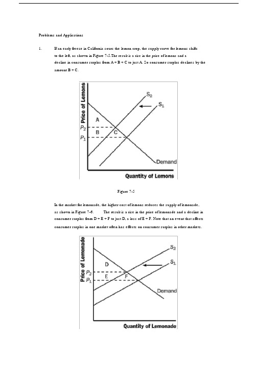
Problems and Applications1.If an early freeze in California sours the lemon crop, the supply curve for lemons shiftsto the left, as shown in Figure 7-5.The result is a rise in the price of lemons and adecline in consumer surplus from A + B + C to just A. So consumer surplus declines by the amount B + C.Figure 7-5In the market for lemonade, the higher cost of lemons reduces the supply of lemonade,as shown in Figure 7-6.The result is a rise in the price of lemonade and a decline inconsumer surplus from D + E + F to just D, a loss of E + F. Note that an event that affectsconsumer surplus in one market often has effects on consumer surplus in other markets.Figure 7-62. A rise in the demand for French bread leads to an increase in producer surplus in themarket for French bread, as shown in Figure 7-7.The shift of the demand curve leads to an increased price, which increases producer surplus from area A to area A + B + C.Figure 7-7The increased quantity of French bread being sold increases the demand for flour, asshown in Figure 7-8.As a result, the price of flour rises, increasing producer surplusfrom area D to D + E + F. Note that an event that affects producer surplus in onemarket leads to effects on producer surplus in related markets.Figure 7-83. a.Bert’ s demand schedule is:Price Quantity DemandedMore than $7 0$5 to $7 1$3 to $5 2$1 to $3 3$1 or less 4Bert’ s demand curve is shown in Figure 7 -9.Figure 7-9b.When the price of a bottle of water is $4, Bert buys two bottles of water.Hisconsumer surplus is shown as area A in the figure.He values his first bottle ofwater at $7, but pays only $4 for it, so has consumer surplus of $3.He valueshis second bottle of water at $5, but pays only $4 for it, so has consumersurplus of $1.Thus Bert’ s total consumer surplus is $3 + $1 = $4, which isthe area of A in the figure.c.When the price of a bottle of water falls from $4 to $2, Bert buys three bottlesof water, an increase of one. His consumer surplus consists of both areas Aand B in the figure, an increase in the amount of area B. He gets consumersurplus of $5 from the first bottle ($7 value minus $2 price), $3 from thesecond bottle ($5 value minus $2 price), and $1 from the third bottle ($3 valueminus $2 price), for a total consumer surplus of $9. Thus consumer surplusrises by $5 (which is the size of area B) when the price of a bottle of water fallsfrom $4 to $2.4. a. Ernie ’ s supply schedule for water is:Price Quantity SuppliedMore than $7 4$5 to $7 3$3 to $5 2$1 to $3 1Less than $1 0Ernie’ s supply curve is shown in Figure 7 -10.Figure 7-10b.When the price of a bottle of water is $4, Ernie sells two bottles of water.Hisproducer surplus is shown as area A in the figure.He receives $4 for his firstbottle of water, but it costs only $1 to produce, so Ernie has producer surplusof $3.He also receives $4 for his second bottle of water, which costs $3 toproduce, so he has producer surplus of$1. Thus Ernie’ s total producersurplus is $3 + $1 = $4, which is the area of A in the figure.c.When the price of a bottle of water rises from $4 to $6, Ernie sells three bottlesof water, an increase of one.His producer surplus consists of both areas Aand B in the figure, an increase by the amount of area B.He gets producersurplus of $5 from the first bottle ($6 price minus $1 cost), $3 from the secondbottle ($6 price minus $3 cost), and $1 from the third bottle ($6 price minus $5price), for a total producer surplus of $9.Thus producer surplus rises by $5(which is the size of area B) when the price of a bottle of water rises from $4to $6.5. a. From Ernie ’ s supply schedule and Bert ’ s demand schedule, the quantitydemanded and supplied are:Price Quantity Supplied Quantity Demanded$ 2 1 34 2 26 3 1Only a price of $4 brings supply and demand into equilibrium, withan equilibrium quantity of 2.b.At a price of $4, consumer surplus is $4 and producer surplus is $4, as shownin problems 3 and 4.Total surplus is $4 + $4 = $8.c.If Ernie produced one fewer bottle, his producer surplus would decline to $3,as shown in problem 4.If Bert consumed one fewer bottle, his consumersurplus would decline to $3, as shown in problem 3. So total surplus would declineto $3 + $3 = $6.d.If Ernie produced one additional bottle of water, his cost would be $5, but theprice is only $4, so his producer surplus would decline by $1.If Bertconsumed one additional bottle of water, his value would be $3, but the priceis $4, so his consumer surplus would decline by $1.So total surplus declinesby $1 + $1 = $2.6. a.The effect of falling production costs in the market for stereos results in a shiftto the right in the supply curve, as shown in Figure 7-11.As a result, theequilibrium price of stereos declines and the equilibrium quantity increases.b.The decline in the price of stereos increases consumer surplus from area A to A+ B + C + D, an increase in the amount B + C + D.Prior to the shift in supply,producer surplus was areas B + E (the area above the supply curve and belowthe price).After the shift in supply, producer surplus is areas E + F + G.Soproducer surplus changes by the amount F + G - B, which may be positive ornegative.The increase in quantity increases producer surplus, while thedecline in the price reduces producer surplus.Since consumer surplus risesby B + C + D and producer surplus rises by F + G - B, total surplus rises by C+ D+F+G.c.If the supply of stereos is very elastic, then the shift of the supply curvebenefits consumers most.To take the most dramatic case, suppose thesupply curve were horizontal, as shown in Figure 7-12.Then there is noproducer surplus at all.Consumers capture all the benefits of fallingproduction costs, with consumer surplus rising from area A to area A + B.Figure 7-11Figure 7-127. Figure 7-13 shows supply and demand curves for haircuts. Supply equals demand ata quantity of three haircuts and a price between $4 and $5. Firms A, C, and D shouldcut the hair of Sally Jessy, Jerry, and Montel. Oprah ’ s willingness to pay is too low and firm B ’ s costs are too high, so they do not participate. The maximum total surplus isthe area between the demand and supply curves, which totals $11 ($8 value minus$2 cost for the first haircut, plus $7 value minus $3 cost for the second, plus $5 valueminus $4 cost for the third).Figure 7-138. a.The effect of falling production costs in the market for computers results in ashift to the right in the supply curve, as shown in Figure 7-14.As a result, theequilibrium price of computers declines and the equilibrium quantity increases.The decline in the price of computers increases consumer surplus from area Ato A + B + C + D, an increase in the amount B + C + D.Figure 7-14Prior to the shift in supply, producer surplus was areas B + E (the area abovethe supply curve and below the price).After the shift in supply, producersurplus is areas E + F + G.So producer surplus changes by the amount F + G- B, which may be positive or negative.The increase in quantity increasesproducer surplus, while the decline in the price reduces producer surplus. Sinceconsumer surplus rises by B + C + D and producer surplus rises by F + G - B,total surplus rises by C + D + F + G.——Figure 7-15b.Since adding machines are substitutes for computers, the decline in the priceof computers means that people substitute computers for adding machines,shifting the demand for adding machines to the left, as shown in Figure 7-15.The result is a decline in both the equilibrium price and equilibrium quantity ofadding machines.Consumer surplus in the adding-machine market changesfrom area A + B to A + C, a net gain of C - B.Producer surplus changes fromarea C + D + E to area E, a net loss of C + D.Adding machine producers aresad about technological advance in computers because their producersurplus declines.c.Since software and computers are complements, the decline in the price andincrease in the quantity of computers means that people’ s demand forsoftware increases, shifting the demand for software to the right, as shown inFigure 7-16. The result is an increase in both the price and quantity of software.Consumer surplus in the software market changes from B + C to A+B, a net increase of A - C. Producer surplus changes from E to C + D + E, anincrease of C + D, so software producers should be happy about the technologicalprogress in computers.d.Yes, this analysis helps explain why Bill Gates is one the world’ s richest msince his company produces a lot of software that’ s a complement withcomputers and there has been tremendous technological advance incomputers.——Figure 7-169. a. Figure 7-17 illustrates the demand for medical care. If each procedure has aprice of $100, quantity demanded will be Q 1 procedures.Figure 7-17b.If consumers pay only $20 per procedure, the quantity demanded will be Q 2procedures.Since the cost to society is $100, the number of proceduresperformed is too large to maximize total surplus.The quantity thatmaximizes total surplus is Q 1 procedures, which is less than Q2.c.The use of medical care is excessive in the sense that consumers getprocedures whose value is less than the cost of producing them.As a result,——the economy’ s total surplus is reduced.d.To prevent this excessive use, the consumer must bear the marginal cost ofthe procedure.But this would require eliminating insurance.Anotherpossibility would be that the insurance company, which pays most of themarginal cost of the procedure ($80, in this case) could decide whether theprocedure should be performed.But the insurance company doesn’ t get thebenefits of the procedure, so its decisions may not reflect the value to theconsumer.10. a. Figure 7-18 illustrates the effect of the drought. The supply curve shifts tothe left, leading to a rise in the equilibrium price from P 1 to P 2 and a decline inthe equilibrium quantity from Q 1 to Q 2 .Figure 7-18b.If the price of water is not allowed to change, there will be an excess demandfor water, with the shortage shown on the figure as the difference between Q 1and Q 3 .c.The system for allocating water is inefficient because it no longer allocateswater to those who value it most highly.Some people who value water atmore than its cost of production will be unable to obtain it, so societysurplus isn’ t maximized.The allocation system seems unfair as well.Water is allocated simply on pastusage, rewarding past wastefulness.If a family’ s demand for water increases,——say because of an increase in family size, the policy doesn ’ t allow them to obtain more water. Poor families, who probably used water mostly fornecessary uses like drinking, would suffer more than wealthier families whowould have to cut back only on luxury uses of water like operating backyardfountains and pools. However, the policy also keeps the price of water lower,which benefits poor families, since otherwise more of their family budgetwould have to go for water.d. If the city allowed the price of water to rise to its equilibrium price P 2 , theallocation would be more efficient. Quantity supplied would equal quantitydemanded and there would be no shortage. Total surplus would bemaximized.Whether the market allocation would be more or less fair than theproportionate reduction in water under the old policy is difficult to say, but it islikely to be more fair. Notice that the quantity supplied would be higher (Q 2)in this case than under the water restrictions (Q 3 ), so there ’ s less reduction inwater usage. To make the market solution even more fair, the governmentcould provide increased tax relief or welfare payments for poor families whosuffer from paying the higher water prices.。

曼昆经济学习题解答

曼昆经济学习题解答Ch5 经济增长2⼀、名词解释劳动效率劳动扩⼤型技术进步内⽣增长理论⼆、选择题1．在有⼈⼝增长和技术进步的索洛模型中，稳定状态时每个效率⼯⼈的产出增长率等于：（）A．0 B．技术增长率gC．⼈⼝增长率n＋技术增长率g D．储蓄率s2．在有⼈⼝增长和技术进步的索洛模型中，稳定状态时每个⼯⼈的产出增长率等于：（）A．0 B．技术增长率gC．⼈⼝增长率n＋技术增长率g D．储蓄率s3．在⼈⼝增长⽐率为n和劳动扩⼤型技术进步⽐率为g的索洛模型中，每个效率⼯⼈的资本存量变化等于：（）A．sf(k) + (d + n + g)k B．sf(k) + (d - n - g)kC．sf(k) - (d + n + g)k D．sf(k) - (d - n - g)k4．下列可以⿎励技术进步的是（）A．新产品实⾏专利制度B．对研发的税收激励C．对研发的政府补贴D．以上都是5．索洛模型表明⾼⼈⼝增长率的国家将会有（）：A．较低的稳定状态⼈均产出⽔平B．较低的稳定状态⼈均产出增长率C．A和B D．较⾼的稳定状态⼈均产出增长率三、问答题1．政府政策为医学研究提供资⾦是⼀个经常被争论的问题。

a.运⽤外部性，社会收益和私⼈收益的概念，讨论政府为什么应该或者不应该为医学研究提供资⾦。

政府怎样才能⿎励私营公司增加研究开⽀？b.如果政府觉得需要对医学研究投⼊更⼤的资⾦，你认为政府是直接投资研究项⽬还是对投资这些研究私营公司采⽤激励政策更好？你认为这两个计划分别会对药品⽣产所产⽣的费⽤发⽣怎样的影响？2．⽐较两部门内⽣增长模型和索洛模型。

两个模型的相同之处是什么？两个模型的假设有不同？你觉得哪个更实际？请解释。

3．在索洛模型中，谈谈技术进步、资本存量的增长、⼈⼝的增长对稳定状态的⼈均收⼊增长率的影响？4．为了确定⼀个经济的资本⼤于还是⼩于黄⾦规则稳定状态，你需要什么数据？5．决策者可以如何影响⼀国的储蓄率？6．过去40年间⽣产率的增长率发⽣了什么变动？你如何解释这种现象、7．内⽣增长理论如何在没有外⽣技术进步的假设的情况下解释长期增长？这种解释与索洛模型有什么不同？8．证明下列有关⼈⼝增长与技术进步时稳定状态的每⼀种表述。

1、下载文档前请自行甄别文档内容的完整性，平台不提供额外的编辑、内容补充、找答案等附加服务。
2、"仅部分预览"的文档,不可在线预览部分如存在完整性等问题,可反馈申请退款(可完整预览的文档不适用该条件!)。
3、如文档侵犯您的权益，请联系客服反馈,我们会尽快为您处理(人工客服工作时间：9:00-18:30)。

Answers to Textbook Questions and ProblemsCHAPTER 7 Unemployment and the Labor MarketQuestions for Review1. The rates of job separation and job finding determine the natural rate of unemployment. The rate of jobseparation is the fraction of people who lose their job each month. The higher the rate of job separation, the higher the natural rate of unemployment. The rate of job finding is the fraction of unemployed people who find a job each month. The higher the rate of job finding, the lower the natural rate ofunemployment.2. Frictional unemployment is the unemployment caused by the time it takes to match workers and jobs.Finding an appropriate job takes time because the flow of information about job candidates and job vacancies is not instantaneous. Because different jobs require different skills and pay different wages, unemployed workers may not accept the first job offer they receive.In contrast, structural unemployment is the unemployment resulting from wage rigidity and job rationing. These workers are unemployed not because they are actively searching for a job that best suits their skills (as in the case of frictional unemployment), but because at the prevailing real wage the quantity of labor supplied exceeds the quantity of labor demanded. If the wage does not adjust to clear the labor market, then these workers must wait for jobs to become available. Structural unemployment thus arises because firms fail to reduce wages despite an excess supply of labor.3. The real wage may remain above the level that equilibrates labor supply and labor demand because ofminimum wage laws, the monopoly power of unions, and efficiency wages.Minimum-wage laws cause wage rigidity when they prevent wages from falling to equilibrium levels. Although most workers are paid a wage above the minimum level, for some workers, especially the unskilled and inexperienced, the minimum wage raises their wage above the equilibrium level. It therefore reduces the quantity of their labor that firms demand, and creates an excess supply ofworkers, which increases unemployment.The monopoly power of unions causes wage rigidity because the wages of unionized workers are determined not by the equilibrium of supply and demand but by collective bargaining between union leaders and firm management. The wage agreement often raises the wage above the equilibrium level and allows the firm to decide how many workers to employ. These high wages cause firms to hire fewer workers than at the market-clearing wage, so structural unemployment increases.Efficiency-wage theories suggest that high wages make workers more productive. The influence of wages on worker efficiency may explain why firms do not cut wages despite an excess supply of labor. Even though a wage reduction decreases the firm’s wage bill, it may also lower workerproductivity and therefore the firm’s profits.4. Depending on how one looks at the data, most unemployment can appear to be either short term orlong term. Most spells of unemployment are short; that is, most of those who became unemployed find jobs quickly. On the other hand, most weeks of unemployment are attributable to the small number of long-term unemployed. By definition, the long-term unemployed do not find jobs quickly, so they appear on unemployment rolls for many weeks or months.5. Europeans work fewer hours than Americans. One explanation is that the higher income tax rates inEurope reduce the incentive to work. A second explanation is a larger underground economy in Europe as a result of more people attempting to evade the high tax rates. A third explanation is the greater importance of unions in Europe and their ability to bargain for reduced work hours. A final explanation is based on preferences, whereby Europeans value leisure more than Americans do, and therefore elect to work fewer hours.Problems and Applications1. a. In the example that follows, we assume that during the school year you look for a part-time job,and that, on average, it takes 2 weeks to find one. We also assume that the typical job lasts 1semester, or 12 weeks.b. If it takes 2 weeks to find a job, then the rate of job finding in weeks isf = (1 job/2 weeks) = 0.5 jobs/week.If the job lasts for 12 weeks, then the rate of job separation in weeks iss = (1 job/12 weeks) = 0.083 jobs/week.c. From the text, we know that the formula for the natural rate of unemployment is(U/L) = [s/(s + f )],where U is the number of people unemployed, and L is the number of people in the labor force.Plugging in the values for f and s that were calculated in part (b), we find(U/L) = [0.083/(0.083 + 0.5)] = 0.14.Thus, if on average it takes 2 weeks to find a job that lasts 12 weeks, the natural rate ofunemployment for this population of college students seeking part-time employment is 14 percent.2. Call the number of residents of the dorm who are involved I, the number who are uninvolved U, and thetotal number of students T = I + U. In steady state the total number of involved students is constant.For this to happen we need the number of newly uninvolved students, (0.10)I, to be equal to thenumber of students who just became involved, (0.05)U. Following a few substitutions:(0.05)U = (0.10)I= (0.10)(T – U),soWe find that two-thirds of the students are uninvolved.3. To show that the unemployment rate evolves over time to the steady-state rate, let’s begin by defininghow the number of people unemployed changes over time. The change in the number of unemployed equals the number of people losing jobs (sE) minus the number finding jobs (fU). In equation form, we can express this as:U t + 1–U t= ΔU t + 1 = sE t–fU t.Recall from the text that L = E t + U t, or E t = L –U t, where L is the total labor force (we will assume that L is constant). Substituting for E t in the above equation, we findΔU t + 1 = s(L –U t) –fU t.Dividing by L, we get an expression for the change in the unemployment rate from t to t + 1:ΔU t + 1/L = (U t + 1/L) – (U t/L) = Δ[U/L]t + 1 = s(1 –U t/L) –fU t/L.Rearranging terms on the right side of the equation above, we end up with line 1 below. Now take line1 below, multiply the right side by (s + f)/(s + f) and rearrange terms to end up with line2 below:Δ[U/L]t + 1= s – (s + f)U t/L= (s + f)[s/(s + f) – U t/L].The first point to note about this equation is that in steady state, when the unemployment rate equals its natural rate, the left-hand side of this expression equals zero. This tells us that, as we found in the text, the natural rate of unemployment (U/L)n equals s/(s + f). We can now rewrite the above expression, substituting (U/L)n for s/(s + f), to get an equation that is easier to interpret:Δ[U/L]t + 1 = (s + f)[(U/L)n–U t/L].This expression shows the following:•If U t/L > (U/L)n (that is, the unemployment rate is above its natural rate), then Δ[U/L]t + 1 is negative: the unemployment rate falls.•If U t/L < (U/L)n (that is, the unemployment rate is below its natural rate), then Δ[U/L]t + 1 is positive: the unemployment rate rises.This process continues until the unemployment rate U/L reaches the steady-state rate (U/L)n.4. Consider the formula for the natural rate of unemployment,If the new law lowers the chance of separation s, but has no effect on the rate of job finding f, then the natural rate of unemployment falls.For several reasons, however, the new law might tend to reduce f. First, raising the cost of firing might make firms more careful about hiring workers, since firms have a harder time firing workers who turn out to be a poor match. Second, if job searchers think that the new legislation will lead them to spend a longer period of time on a particular job, then they might weigh more carefully whether or not to take that job. If the reduction in f is large enough, then the new policy may even increase the natural rate of unemployment.5. a. The demand for labor is determined by the amount of labor that a profit-maximizing firm wants tohire at a given real wage. The profit-maximizing condition is that the firm hire labor until themarginal product of labor equals the real wage,The marginal product of labor is found by differentiating the production function with respect tolabor (see Chapter 3 for more discussion),In order to solve for labor demand, we set the MPL equal to the real wage and solve for L:Notice that this expression has the intuitively desirable feature that increases in the real wagereduce the demand for labor.b. We assume that the 27,000 units of capital and the 1,000 units of labor are supplied inelastically(i.e., they will work at any price). In this case we know that all 1,000 units of labor and 27,000 units of capital will be used in equilibrium, so we can substitute these values into the above labor demand function and solve for .In equilibrium, employment will be 1,000, and multiplying this by 10 we find that the workers earn 10,000 units of output. The total output is given by the production function:Y=5K 13L23Y=5(27,00013)(1,00023)Y=15,000.Notice that workers get two-thirds of output, which is consistent with what we know about theCobb–Douglas production function from Chapter 3.c. The real wage is now equal to 11 (10% above the equilibrium level of 10).Firms will use their labor demand function to decide how many workers to hire at the given realwage of 11 and capital stock of 27,000:So 751 workers will be hired for a total compensation of 8,261 units of output. To find the newlevel of output, plug the new value for labor and the value for capital into the production function and you will find Y = 12,393.d. The policy redistributes output from the 249 workers who become involuntarily unemployed tothe 751 workers who get paid more than before. The lucky workers benefit less than the losers lose as the total compensation to the working class falls from 10,000 to 8,261 units of output.e. This problem does focus on the analysis of two effects of the minimum-wage laws: they raise thewage for some workers while downward-sloping labor demand reduces the total number of jobs.Note, however, that if labor demand is less elastic than in this example, then the loss ofemployment may be smaller, and the change in worker income might be positive.6. a. The labor demand curve is given by the marginal product of labor schedule faced by firms. If acountry experiences a reduction in productivity, then the labor demand curve shifts to the left as in Figure 7-1. If labor becomes less productive, then at any given real wage, firms demand less labor.b. If the labor market is always in equilibrium, then, assuming a fixed labor supply, an adverseproductivity shock causes a decrease in the real wage but has no effect on employment orunemployment, as in Figure 7-2.c. If unions constrain real wages to remain unaltered, then as illustrated in Figure 7-3, employmentfalls to L1 and unemployment equals L –L1.This example shows that the effect of a productivity shock on an economy depends on the role of unions and the response of collective bargaining to such a change.7. a. If workers are free to move between sectors, then the wage in each sector will be equal. If thewages were not equal then workers would have an incentive to move to the sector with the higher wage and this would cause the higher wage to fall, and the lower wage to rise until they wereequal.b. Since there are 100 workers in total, L S = 100 – L M. We can substitute this expression into thelabor demand for services equation, and call the wage w since it is the same in both sectors:L S = 100 – L M = 100 – 4wL M = 4w.Now set this equal to the labor demand for manufacturing equation and solve for w:4w = 200 – 6ww = $20.Substitute the wage into the two labor demand equations to find L M is 80 and L S is 20.c. If the wage in manufacturing is equal to $25 then L M is equal to 50.d. There are now 50 workers employed in the service sector and the wage w S is equal to $12.50.e. The wage in manufacturing will remain at $25 and employment will remain at 50. If thereservation wage for the service sector is $15 then employment in the service sector will be 40.Therefore, 10 people are unemployed and the unemployment rate is 10 percent.8. Real wages have risen over time in both the United States and Europe, increasing the reward forworking (the substitution effect) but also making people richer, so they want to “buy” more leisure (the income effect). If the income effect dominates, then people want to work less as real wages go up. This could explain the European experience, in which hours worked per employed person have fallen over time. If the income and substitution effects approximately cancel, then this could explain the U.S.experience, in which hours worked per person have stayed about constant. Economists do not havegood theories for why tastes might differ, so they disagree on whether it is reasonable to think that Europeans have a larger income effect than do Americans.9. The vacant office space problem is similar to the unemployment problem; we can apply the sameconcepts we used in analyzing unemployed labor to analyze why vacant office space exists. There is a rate of office separation: firms that occupy offices leave, either to move to different offices or because they go out of business. There is a rate of office finding: firms that need office space (either to start up or expand) find empty offices. It takes time to match firms with available space. Different types of firms require spaces with different attributes depending on what their specific needs are. Also, because demand for different goods fluctuates, there ar e “sectoral shifts”—changes in the composition of demand among industries and regions that affect the profitability and office needs of different firms.。

曼昆-宏观经济经济学第九版-英文原版答案7

曼昆微观经济学课后练习英文答案(第七章)

国际经济学第九版英文课后答案解析第7单元

曼昆宏观经济经济学第九版英文原版答案

曼昆经济学原理7-9

曼昆宏观经济经济学第九版英文原版答案

(完整word版)国际经济学第九版英文课后答案 第7单元

经济学原理曼昆课后答案chapter7.doc

曼昆经济学习题解答

(完整word版)国际经济学第九版英文课后答案第7单元