A note on common zeroes of Laplace--Beltrami eigenfunctions
laplace
F (s)est ds
σ−j∞
where σ is large enough that F (s) is defined for
s≥σ
surprisingly, this formula isn’t really useful!
The Laplace transform
3–13
Time scaling
3–1
Idea
the Laplace transform converts integral and differential equations into algebraic equations this is like phasors, but • applies to general signals, not just sinusoids • handles non-steady-state conditions allows us to analyze • LCCODEs • complicated circuits with sources, Ls, Rs, and Cs • complicated systems with integrators, differentiators, gains
2 = 3− s−1 3s − 5 = s−1
The Laplace transform
3–10
One-to-one property
the Laplace transform is one-to-one: if L(f ) = L(g) then f = g
(well, almost; see below)
=1 s)t
e−(
s)t
= e−(
s)t
• the integral defining F makes sense for all s with
F q Set of q Alphabets
: : : : : : : : : : : : : : : : : : : : : : : : : : : :
ˆk Generator matrix of S r th -order Reed M¨ uller Code Binary nonlinear Preparata Code Binary nonlinear Kerdock Code max{M | there exists a binary (n, M, dH ) code } Gray map {φ(c) : c ∈ C} : Gray image of C Irreducible polynomial over Z2 such that it divides xn − 1 over Z2 Hensel uplift of h2 (x) over Z4 p-basis of C p-dimension of C Generalized gray map Generalized gray image of C Generalized gray image of C in 2-basis form Binary residue code of C Binary torsion code of C Correlation of c ∈ C Simplex Code of type α Simplex Code of type β
Synopsis
Name of the student: Manish Kumar Gupta Degree for which submitted: Ph.D. Thesis Title: On Some Linear Codes over Z2s Name of the Thesis Supervisors: Prof. M. C. Bhandari & Prof. A. K. Lal Month and Year of Thesis Submission: December, 1999 Roll No.: 9310863 Department: Mathematics
Redundant Picard-Fuchs system for Abelian integrals
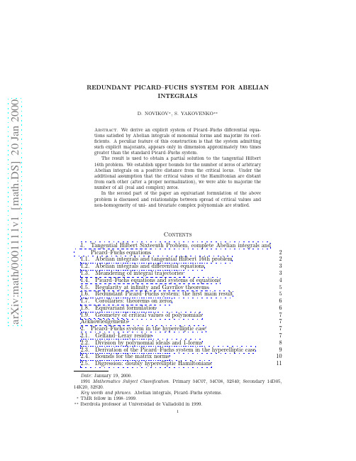
a rX iv:mat h /1111v1[mat h.DS]2Ja n2REDUNDANT PICARD–FUCHS SYSTEM FOR ABELIAN INTEGRALS D.NOVIKOV ∗,S.YAKOVENKO ∗∗Abstract.We derive an explicit system of Picard–Fuchs differential equa-tions satisfied by Abelian integrals of monomial forms and majorize its coef-ficients.A peculiar feature of this construction is that the system admitting such explicit majorants,appears only in dimension approximately two times greater than the standard Picard–Fuchs system.The result is used to obtain a partial solution to the tangential Hilbert 16th problem.We establish upper bounds for the number of zeros of arbitrary Abelian integrals on a positive distance from the critical locus.Under the additional assumption that the critical values of the Hamiltonian are distant from each other (after a proper normalization),we were able to majorize the number of all (real and complex)zeros.In the second part of the paper an equivariant formulation of the above problem is discussed and relationships between spread of critical values and non-homogeneity of uni-and bivariate complex polynomials are studied.Contents 1.Tangential Hilbert Sixteenth Problem,complete Abelian integrals and Picard–Fuchs equations 21.1.Abelian integrals and tangential Hilbert 16th problem 21.2.Abelian integrals and differential equations 31.3.Meandering of integral trajectories 31.4.Picard–Fuchs equations and systems of equations 41.5.Regularity at infinity and Gavrilov theorems 51.6.Redundant Picard–Fuchs system:the first main result 51.7.Corollaries:theorems on zeros 61.8.Equivariant formulation 61.9.Geometry of critical values of polynomials 7Acknowledgements72.Picard–Fuchs system in the hyperelliptic case72.1.Gelfand–Leray residue72.2.Division by polynomial ideals and 1-forms82.3.Derivation of the Picard–Fuchs system in the hyperelliptic case92.4.Bounds for the matrix norms102.5.Digression:doubly hyperelliptic Hamiltonians112 D.NOVIKOV,S.YAKOVENKO2.6.Discussion123.Derivation of the redundant Picard–Fuchs system123.1.Notations and conventions123.2.Normalizing conditions and quasimonic Hamiltonians133.3.Balanced Hamiltonians133.4.Lemma on bounded division143.5.Derivation of the redundant Picard–Fuchs system153.6.Abelian integrals of higher degrees173.7.Properties of the redundant Picard–Fuchs system174.Zeros of Abelian integrals away from the singular locus and relatedproblems on critical values of polynomials194.1.Heuristic considerations194.2.Meandering theorem and upper bounds for zeros of Abelian integrals204.3.Affine group action and equivariant problem on zeros of Abelianintegrals224.4.From Theorem3to Equivariant problem225.Critical values of polynomials235.1.Geometric consequences of quasimonicity235.2.Almost-homogeneity implies close critical values245.3.Dual formulation,limit and existential problems245.4.Parallel problems for univariate polynomials265.5.Spread of roots vs.spread of critical values for univariate moniccomplex polynomials265.6.Demonstration of Theorem5285.7.Existential bounds cannot be uniform295.8.Discussion:atypical values and singular perturbations29References301.Tangential Hilbert Sixteenth Problem,complete Abelianintegrals and Picard–Fuchs equations The main result of this paper is an explicit derivation of the Picard–Fuchs system of linear ordinary differential equations for integrals of polynomial1-forms over level curves of a polynomial in two variables,regular at infinity.The explicit character of the construction makes it possible to derive upper bounds for the coefficients of this system.In turn,application of the bounded meandering principle[17,15]to the system of differential equations with bounded coefficients allows to produce upper bounds for the number of complex isolated zeros of these integrals on a positive distance from the ramification locus.1.1.Abelian integrals and tangential Hilbert16th problem.If H(x,y)isa polynomial in two real variables,called the Hamiltonian,andω=P(x,y)dx+ Q(x,y)dy a real polynomial1-form,then the problem on limit cycles appearing in the perturbation of the Hamiltonian equation,dH+εω=0,ε∈(R,0)(1.1)REDUNDANT PICARD–FUCHS SYSTEM FOR ABELIAN INTEGRALS3 after linearization inε(whence the adjective“tangential”)reduces to the study of complete Abelian integralI(t)=I(t;H,ω)= H=tω,(1.2) where the integration is carried over a continuous family of(real)ovals lying on the level curves{H=t}.Problem1(Tangential Hilbert16th problem).Place an upper bound for the num-ber of real zeros of the Abelian integral I(t;H,ω)on the maximal natural domain of definition of this integral,in terms of deg H and degω=max(deg P,deg Q)+1.A more natural version appears after complexification.For an arbitrary complex polynomial H(x,y)having only isolated critical points,and an arbitrary complex polynomial1-formω,the integral(1.2)can be extended as a multivalued analytic function ramified over afinite set of points(typically consisting of critical values of H).The problem is to place an upper bound for the number of isolated complex roots of any branch of this function,in terms of deg H and degω.1.2.Abelian integrals and differential equations.Despite its apparently alge-braic character,the tangential Hilbert problem still resists all attempts to approach it using methods of algebraic geometry.Almost all progress towards its solution so far was based on using methods of analytic theory of differential equations.In particular,the(existential)generalfiniteness theorem by Khovanski˘ı–Var-chenko[12,24]claims that for anyfinite combination of d=degωand n=deg H the number of isolated zeros is indeed uniformly bounded over all forms and all Hamiltonians of the respective degree.One of the key ingredients of the proof is the so called Pfaffian elimination,an analog of the intersection theory for varieties defined by Pfaffian differential equations[13].Another important achievement,an explicit upper bound for the number of zeros in the elliptic case when H(x,y)=y2+p(x),deg p=3and forms of arbitrary degree,due to G.Petrov[21],uses the fact that the elliptic integrals I k(t)= x k−1y dx,k=1,2,in this case satisfy an explicit system of linearfirst order system of differential equations with rational coefficients.This method was later generalized for other classes of Hamiltonians whose level curves are elliptic (i.e.,of genus1),see[10,7,27]and references therein.The ultimate achievement in this direction is a theorem by Petrov and Khovanskii,placing an asymptotically linear in degωupper bound for the number of zeros of arbitrary Abelian integrals, with the constants being uniform over all Hamiltonians of degree n(unpub-lished).However,one of these constants is purely existential:its dependence on n is totally unknown.It is important to remark that all the approaches mentioned above,require a very basic and easily obtainable information concerning the differential equations(their mere existence,types of singularities,polynomial or rational form of coefficients,in some cases their degree).1.3.Meandering of integral trajectories.A different approach suggested in [14]consists in an attempt to apply a very general principle,according to which integral trajectories of a polynomial vectorfield(in R n or C n)have a controllable meandering(sinuosity),[17,15].More precisely,if a curve of known size is a part of an integral trajectory of a polynomial vectorfield whose degree and the magnitude4 D.NOVIKOV,S.YAKOVENKOof the coefficients are explicitly bounded from above,then the number of isolated intersections between this curve and any affine hyperplane in the ambient space can be explicitly majorized in terms of these data.The bound appears to be very excessive:it is polynomial in the size of the curve and the magnitude of the coefficients,but the exponent as the function of the degree and the dimension of the ambient space,grows as a tower(iterated exponent)of height4.In order to apply this principle to the tangential Hilbert problem,we consider the curve parameterized by the monomial integrals,t→(I1(t),...,I N(t)),I i(t)= H=tωi,whereωi,i=1,...,N are all monomial forms of degree d.Isolated zeros of the Abelian integral of an arbitrary polynomial1-formω= i c iωi correspond to isolated intersections of the above curve with the hyperplane c i I i=0.If this monomial curve is integral for a system of polynomial differential equations with explicitly bounded coefficients,then the bounded meandering principle would yield a(partial)answer for the tangential Hilbert16th problem.The system of polynomial(in fact,linear)differential equations can be written explicitly for the case of hyperelliptic integrals corresponding to the Hamiltonian H(x,y)=y2+p(x)with an arbitrary univariate potential p(x)∈C[x],see§2below and references therein.Application of the bounded meandering principle allowed us to prove in[14]that the number of zeros of hyperelliptic integrals is majorized by a certain tower function depending only on the degrees of n=deg H=deg p and d=degω.(Actually,it was done under an additional assumption that all critical values of p are real,but we believe that this restriction is technical and can be removed).1.4.Picard–Fuchs equations and systems of equations.In order to general-ize the construction from[14]for the case of arbitrary(not necessarily hyperelliptic) Hamiltonians it is necessary,among other things,to write a system of polynomial differential equations for Abelian integrals and estimate explicitly the magnitude of its coefficients.The mere existence of such a system is well known since times of Riemann if not Gauss.In today’s language,the monodromy group of any form depends only on the Hamiltonian.Denote byµthe rank of thefirst homology group of a typical affine level curve{H=t}⊂C2.Then for any collection of1-formsω1,...,ωµthe period matrix X(t)can be formed,whose entries are integrals ofωi over the cycles δ1(t),...,δµ(t)generating the homology.If the determinant of this matrix if not identically zero,then X(t)satisfies a linear ordinary differential equation of the form˙X(t)=A(t)X(t),A(·)∈Mat(C(t)),(1.3)µ×µwith a rational matrix function A(t).This system of equations is known under several names,from Gauss–Manin connection[20,especially p.18]to Picard–Fuchs system(of linear ordinary differential equations with rational coefficients,in full). We shall systematically use the last name.The rank of thefirst homology can be easily computed:for a generic Hamiltonian of degree n+1it is equal to n2.The degree deg A(t)can be relatively easily determined if the degrees of the formsωi are known.However,the choice of the formsωi may also be a difficult problem for some Hamiltonians.The matrix A(t)REDUNDANT PICARD–FUCHS SYSTEM FOR ABELIAN INTEGRALS5 apriori may have poles not only in the ramification points of the Abelian integrals, which leads to additional difficulties.But worst of all,this topological approach gives absolutely no control over the magnitude of the(matrix)coefficients of the rational(matrix)function A(t).1.5.Regularity at infinity and Gavrilov theorems.Part of these problems problems can be resolved.In particular,if the Hamiltonian is sufficiently regular at infinity,then all questions concerning the degrees,can be answered.Definition1.A polynomial H(x,y)∈C[x,y]of degree n+1is said to be regular at infinity,if one of the three equivalent conditions holds:1.its principal homogeneous part H,a homogeneous polynomial of degree n+1,is a product of n+1pairwise different linear forms;2. H has an isolated critical point(necessarily of multiplicityµ=n2)at theorigin(x,y)=(0,0);3.the level curve{ H=1}⊂C2is nonsingular.This condition means that after the natural projective compactification of the (x,y)-plane C2,all“interesting”things still happen only in thefinite part of the compactified plane.In particular,for a polynomial regular at infinity:1.all level curves{H=t}intersect the infinite line C P1∞⊂C P2transversally,2.all critical points{(x,y):dH(x,y)=0}are isolated and their number isexactlyµ=n2if counted with multiplicities,3.the rank of thefirst homology of any regular affine level curve{H=t}isµ=n2,4.the map H:C2→C1is a topological bundle over the set of the regular valuesof H,hence the Abelian integrals can be ramified only over the critical values of H.In[5]L.Gavrilov proved that for polynomials regular at infinity,the space of Abelian integrals isfinitely generated as a C[t]-module byµbasic integrals that can be chosen as integrals of anyνformsωi of degree 2n whose differentials form the basis of the quotient spaceΛ2/d H∧Λ1,whereΛk is the space of polynomial k-forms on C2.As a corollary,one can prove that the collection of these basic integrals satisfies a system of equations(1.3)of sizeµ×µwithµ=n2,and place an upper bound for the degree of the corresponding matrix function A(t).This system is minimal(irredundant):generically(for Morse Hamiltonians regular at infinity), all branches of full analytic continuation of an Abelian integral span exactlyµ-dimensional linear space.From this theorem one can also derive further information concerning the Picard–Fuchs ly,one can prove that if in addition to being regular at infinity,H is a Morse function on C2,then the matrix A(t)of the Picard–Fuchs system(1.3)has only simple poles(Fuchsian singularities)at the critical values of the Hamiltonian and only at them(the point t=∞is a regular though in general non-Fuchsian singularity).However,these results do not yet allow an explicit majoration of the coefficients(e.g.,the residue matrices)of the matrix function A(t)in(1.3).1.6.Redundant Picard–Fuchs system:thefirst main result.We suggest in this paper a procedure of explicit derivation of the Picard–Fuchs system of equations,based on the division by the gradient ideal H x,H y ⊂C[x,y]in the6 D.NOVIKOV,S.YAKOVENKOpolynomial ring.It turns out that if instead of choosingµ=n2forms of degree 2n constituting a basis modulo the gradient ideal,one takes allν=n(2n−1) cohomologically independent monomial forms of degree 2n,then the resulting Picard–Fuchs system can be written in the form(tE−A)˙X(t)=BX(t),A,B∈Matν×ν(C),(1.4) where E is the identity matrix,and X(t)is the rectangular periodν×µ-matrix.The procedure of deriving the system(1.4),being completely elementary,can be easily analyzed and upper bounds for the matrix norms A and B derived. These bounds depend on the magnitude of the all non-principal terms H− H of the Hamiltonian,relative to the principal part H.More precisely,we introduce a normalizing condition(quasimonicity)on the ho-mogeneous part:this condition plays the same role as the assumption that the leading term has coefficient1for univariate polynomials.The quasimonicity con-dition can be always achieved by an affine change of variables,provided that H is regular at infinity,hence it is not restrictive.Theorem2,ourfirst main result, allows to place an upper bound for the norms A + B in terms of the norm(sum of absolute values of all coefficients)of the non-leading part H− H,assuming thatH is quasimonic.1.7.Corollaries:theorems on zeros.The above information on coefficients of Picard–Fuchs system already suffices to apply the bounded meandering principle and obtain an explicit upper bound for the number of zeros of complete Abelian integrals away from the critical locus of the Hamiltonian(Theorem3),which seems to be thefirst known explicit result of that kind.In addition to this bound valid for some zeros and almost all Hamiltonians,one can apply results(or rather methods)from[22].If in addition to the quasimonicity and bounded lower terms,all critical values t1,...,tµof the Hamiltonian H are far away from each other(i.e.,a lower bound for|t i−t j|is known for i=j),then one can majorize the number of zeros on any branch of the Abelian integral by a function depending only on n,d and the minimal distance between critical values. The accurate formulation is given in Theorem4.1.8.Equivariant formulation.However,the description given by Theorem2, is not completely sufficient for further advance towards solution of the tangential Hilbert problem by studying zeros of Abelian integrals near the critical locus when the latter(or some part of it)shrinks to one point of high multiplicity.One reason is that in order to run an inductive scheme similar to that con-structed in[14],one has to make sure that the Hamiltonian H:C2→C1can be rescaled(using affine transformations in the preimage C2and the image C1)so that simultaneously:1.the critical values of H do not tend to each other(e.g.,their diameter isbounded from below by1),and2.the“non-homogeneous part”H− H is bounded by a constant explicitly de-pending on n(each of the two conditions can be obviously satisfied separately).Another,intrinsic reason is the equivariance(or,rather precisely,non-invariance of neither Theorem2nor Theorems3and4)by the above affine group action.InREDUNDANT PICARD–FUCHS SYSTEM FOR ABELIAN INTEGRALS7 order to be geometrically sound,all assertions should be related to a certain privi-leged affine chart on the t-plane.Since our future goal is to study a neighborhoodof the critical locus,it is natural to choose the privileged chart so that the critical locus will not shrink into one point.More detailed explanations and motivations are given in§4below,where we for-mulate several problems all in the following sense:for a polynomial whose principal homogeneous part is normalized(in a certain sense)and whose critical values are ex-plicitly bounded,it is required to place an upper bound for the“non-homogeneous”part,eventually after a suitable translation(which does not affect the principal part, naturally).1.9.Geometry of critical values of polynomials.The reason why several problems of the above type were formulated instead of just one,is very simple:we do not know a complete solution,so partial,existential or limit cases were con-sidered as intermediate steps towards the ultimate goal.In§5we prove that:•if a monic complex polynomial p(x)=x n+1+···∈C[x]has all critical values in the unit disk,then its roots form a point set of diameter<11(Theorem6)and hence by a suitable translation the norm of the non-principal part can be made 12n+1(this gives a complete solution in the univariate and hyperelliptic cases);•all critical values of a Hamiltonian regular at infinity,cannot simultaneously coincide unless the Hamiltonian is essentially homogeneous(Theorem5);•for any normalized principal part H there exists an upper bound for H− H (eventually after a suitable translation),provided that the critical values ofH are all in the unit disk(Corollary to Theorem5).All these are positive results towards solution of the problem on critical values.It still remains to compute the upper bound from the last assertion explicitly:the proof below does not provide sufficient information for that.However,it can be shown already in simple examples that this bound cannot be uniform over all homogeneous parts.As some of the linear factors from H approach too closely to each other,an explosion occurs and the non-principal part may be arbitrarily large without affecting the“moderate”critical values.The phenomenon can be seen as“almost occurrence”of atypical values,ramification points for Abelian integrals that are not critical values of H:such points are known to appear if the principal part H has a non-isolated singularity. Acknowledgements.We are grateful to J.-P.Fran¸c oise,L.Gavrilov,Yu.Ilya-shenko,A.Khovanskii,man,R.Moussu,R.Roussarie and Y.Yomdin for numerous discussions and many useful remarks.Bernard Teissier suggested an idea thatfinally developed into the proof of Lemma3below.Lucy Moser provided us with a counterexample(§5.6below).We are grateful to all our colleagues from Laboratoire de Topologie,Universit´e de Bourgogne(Dijon)and Departamento de Algebra,Geometr´ıa y Topolog´ıa,Uni-versidad de Valladolid,where a large part of this work has been done.They made our stays and visits very stimulating.2.Picard–Fuchs system in the hyperelliptic case 2.1.Gelfand–Leray residue.The derivative of an Abelian integral H=tωcan be computed as the integral over the same curve of another1-formθcalled the8 D.NOVIKOV,S.YAKOVENKOGelfand–Leray derivative(residue).More precisely,if a pair of polynomial1-forms ω,θsatisfies the identity dω=dH∧θ,then for any continuous family of cyclesδ(t) on the level curves{H=t}dREDUNDANT PICARD–FUCHS SYSTEM FOR ABELIAN INTEGRALS9 2.3.Derivation of the Picard–Fuchs system in the hyperelliptic case. Throughout this section we assume that H(x,y)=12y2+p(x) x i−1dx∧dy= 12x i−1y dx−b i(x)dy∧dH+a i(x)dx∧dy= 12I i+nj=1b ij I j(2.6)or,in the matrix form,(t−A)˙I=BI,I∈C n,A,B∈Mat n×n(C),(2.7) where,obviously,I j(t)= ωj are the Abelian integrals and I=(I1,...,I n)the column vector.10 D.NOVIKOV,S.YAKOVENKORemark1.The computation above does not depend on the choice of the cycle of integration,therefore the system of equations will remain valid if we replace the column vector I by the period matrix X(t)obtained by integrating all formsωi over all vanishing cyclesδj(t),j=1,...,n(see[1])on the hyperelliptic level curves.The matrices A,B can be completely described using the division process(2.3).Let x∗∈C be a critical point of p and t∗=p(x∗)the corresponding critical value.Then(2.3)imply that the column vector(1,x∗,x2∗,...,x n−1∗)∈C n is the eigenvector of A with theeigenvalue t∗,which gives a complete description(eigenbasis and eigenvalues)of A.Entries of the matrix B can be described similarly:b ij=0for j>i because of the assertion about degrees of b j(x),so B is triangular.The diagonal entries can be easily computed by looking at the leading terms:since p is monic,b i(x)=x in+1x i−1+···.Finally,the diagonal entries{−i2}n i=1form the spectrumof B.However,knowledge of the critical values of H is not yet sufficient to produce an upper bound for the norms A , B ,since the conjugacy by the Vandermonde matrix(whosecolumns are the above eigenvectors(1,x j,x2j,...,x n−1j )T,j=1,...,n)may increase ar-bitrarily the norm of the diagonal matrix diag(t1,...,t n),where t j are all critical values of H(or p,what is the same).On the contrary,a linear change in the space of1-forms that makes A diagonal,can increase in an uncontrollable way the norm of the matrix B, whose eigenbasis differs from the standard one by a triangular transformation.It is the explicit division procedure that allows to majorize the matrix norms.2.4.Bounds for the matrix norms.For a polynomial p∈C[x]let p be the sum of absolute values of its coefficients(sometimes it is called the length of p).It has the advantage of being multiplicative, pq p · q .Proposition1.If q=x n+···∈C[x]is a monic polynomial with q−x n =c, then any other polynomial f∈C[x]of degree d n can be divided with remainder,f(x)=b(x)q(x)+a(x),deg a n−1,(2.8)so thatb + a K f ,K=1+C+C2+···+C d−n,C=1+c= q .(2.9) Proof.The proof goes by direct inspection of the Euclid algorithm of univariate polynomial division.The assertion of the Proposition is trivial for q=x n:in this case the string of coefficients of r has to be split into two,and immediately we have the decomposition r=bx n+a with b + a = r .The general nonhomogeneous case is treated by induction.Suppose that the inequality(2.9)is valid for any polynomial f of degree d−1(for d=n−1 it is trivially satisfied by letting b=0and a= f).Take a polynomial f of degree d and write the identity f=bx n+a=bq+b(x n−q)+a=bq+ f, where the polynomial f=a+b(x n−q)is of degree d−1and has the norm explicitly bounded: f c b + a (1+c)( b + a ) C f .By the induction assumption, f can be divided, f= bq+ a,with the norms satisfying the inequality(2.9).Collecting everything together,we have f=(b+ b)q+ a and b+ b + a f +C f (1+C+···+C d−1−n) f (1+···+C d−n).As a corollary to this Proposition and the explicit procedure of the division, we obtain upper bounds for norms of the matrices A,B.Recall that we use theREDUNDANT PICARD–FUCHS SYSTEM FOR ABELIAN INTEGRALS11ℓ1-norm on the“space of columns”,so the norm of a matrix A=(a ij)ni,j=1isA =maxj=1,...,nni=1|a ij|(2.10)Theorem1.Suppose that p(x)=x n+1+ n−1i=0c i x i is a monic polynomial of degree n+1and the non-principal part of p is explicitly bounded: n−1i=0|c i| c.Then the entries of the matrices A,B determining the Picard–Fuchs system(2.7) are explicitly bounded:A +B n2(1+C+···+C n+1),C=1+c= p .(2.11) Proof.The derivative p′(x)is not monic,but the leading coefficient is explicitly known:p′(x)=(n+1)(x n+···) ,with the non-principal part denoted by the dots bounded by c in the sense of the norm.Applying Proposition1to q=p′/(n+1), we see that any polynomial can be divided by p′and the same inequalities(2.9) would hold(since n+1 1).Thus we have b i + a i K x i−1 p =KC,where K=1+C+···+C n,then obviously b′j n b j andfinally for the sum of matrix elements A,B occurring in the i th line,we produce an upper bound12 n(1+C+···+C n+1).Clearly,this means that every entry of thesematrices is majorized by the same expression and therefore for the matrixℓ1-norms on C n we have the required estimate.2.5.Digression:doubly hyperelliptic Hamiltonians.The algorithm suggest-ed above,works with only minor modifications for doubly hyperelliptic Hamiltonians having the form H(x,y)=p(x)+q(y)(the hyperelliptic case corresponds to q(y)= 1∂xy j−∂b∗j12 D.NOVIKOV,S.YAKOVENKObeing a2-form with coefficient of degrees n−1in x and m−1in y,is a linear combination of the forms dωij.Thus we have the equationsH dωij=dH∧ k,l=0B ij,klωkl+dF ij + k,l A ij,kl dωkl,i,k=0,...,n−1,j,l=0,...,m−1.Rescaling x and y by appropriate factors independently,we can assume that the polynomials p(x)and q(y)are both monic.Then all divisions will be bounded pro-vided that the norms p and q are explicitly bounded,and in a way completely similar to the arguments from§2.4,we can derive upper bounds for the matrix coefficients A ij,kl,B ij,kl.Thus the case of doubly hyperelliptic Hamiltonians does not differ much from the ordinary hyperelliptic case,at least as far as the Picard–Fuchs systems for Abelian integrals are concerned.2.6.Discussion.The Picard–Fuchs system written in the form(2.7)for a generic hyperelliptic Hamiltonian(with the potential p(x)being a Morse function on C), is a system remarkable for several instances:•it possesses only Fuchsian singularities(simple poles)both at allfinite singu-larities t=t j,j=1,...,n,and at infinity;•it has no apparent singularities:all points t j are ramification points for the fundamental system of solutions X(t)that is obtained by integrating all forms ωi over all vanishing cyclesδj(t)(the period matrix);•it is minimal in the sense that analytic continuations of any column of the period matrix X(t)along all closed loops span the entire space C n.•its coefficients can be explicitly bounded in terms of H .(All these observations equally apply to doubly hyperelliptic Hamiltonians.) In the next section we generalize this result for arbitrary bivariate Hamiltoni-ans.It will be impossible to preserve all properties,and we shall concentrate on the derivation of redundant system,eventually exhibiting apparent singularities, but all of them(including that at infinity)Fuchsian and with explicitly bounded coefficients.3.Derivation of the redundant Picard–Fuchs system3.1.Notations and conventions.Recall thatΛk denote the spaces of polynomial k-forms on C2for k=0,1,2.They will be always equipped with theℓ1-norms:the norm of a form is always equal to the sum of absolute values of all its coefficients. This norm behaves naturally with respect to the(wedge)product:for any two formsη∈Λk,θ∈Λl,0 k+l 2,we always have η∧θ η · θ .It is also convenient to grade the spaces of polynomial forms so that the degree of a k-form is the maximal degree of its(polynomial)coefficients plus k.Under this convention the exterior derivation is degree-preserving:deg dθ=degθ(unless dθ=0).An easy computation shows that dθ degθ· θ for any0-and1-form θ.On several occasions thefinite-dimensional linear space of k-forms of degree d will be denoted byΛk d.Ifω∈Λ1is a polynomial1-form and H∈Λ0,then by dω/dH is always de-noted the Gelfand–Leray derivative(2.1),while by dω。
拉普拉斯变换及其在机器学习中的应用

The Laplace Transform with Applications in Machine Learning The Laplace Transform Examples
The Laplace Transform with Applications in Machine Learning The Laplace Transform Definition
The Laplace Transform
Suppose that f is a real-or complex-valued function of the variable t ≥ 0. The Laplace transform of function f (t ) is defined by
where Kγ (·) represents the modified Bessel function of the second kind with the index γ . We denote this distribution by GIG(γ, β, α). It is well known that its special cases include the gamma distribution Ga(γ, α/2) when β = 0 and γ > 0, the inverse gamma distribution IG(−γ, β/2) when α = 0 and γ < 0, the inverse Gaussian distribution when γ = −1/2, and the hyperbolic distribution when γ = 0.
The Laplace Transform with Applications in Machine Learning
p-laplace方程 博士文
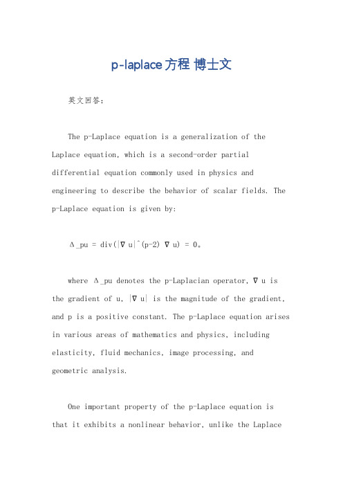
p-laplace方程博士文英文回答:The p-Laplace equation is a generalization of the Laplace equation, which is a second-order partial differential equation commonly used in physics and engineering to describe the behavior of scalar fields. The p-Laplace equation is given by:Δ_pu = div(|∇u|^(p-2) ∇u) = 0。
where Δ_pu denotes the p-Laplacian operator, ∇u is the gradient of u, |∇u| is the magnitude of the gradient, and p is a positive constant. The p-Laplace equation arises in various areas of mathematics and physics, including elasticity, fluid mechanics, image processing, and geometric analysis.One important property of the p-Laplace equation isthat it exhibits a nonlinear behavior, unlike the Laplaceequation. This nonlinearity arises from the power p in the equation, which affects the growth and decay of the solution. For example, when p = 2, the p-Laplace equation reduces to the Laplace equation, and the solution behaves linearly. However, for p ≠ 2, the solution can exhibit different types of nonlinear behavior, such as concentration or diffusion effects.中文回答:p-Laplace方程是Laplace方程的一种推广形式,Laplace方程是一种常见的二阶偏微分方程,常用于描述物理和工程中标量场的行为。
Coordinated path-following of multiple underactuated autonomous vehicles
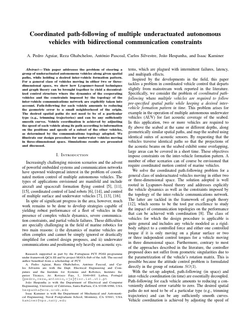
Coordinated path-following of multiple underactuated autonomous vehicles with bidirectional communication constraintsA.Pedro Aguiar,Reza Ghabcheloo,Ant´o nio Pascoal,Carlos Silvestre,Jo˜a o Hespanha,and Isaac KaminerAbstract—This paper addresses the problem of steering a group of underactuated autonomous vehicles along given spatial paths,while holding a desired inter-vehicle formation pattern. For a general class of vehicles moving in either two or three-dimensional space,we show how Lyapunov-based techniques and graph theory can be brought together to yield a decentral-ized control structure where the dynamics of the cooperating vehicles and the constraints imposed by the topology of the inter-vehicle communications network are explicitly taken into account.Path-following for each vehicle amounts to reducing the geometric error to a small neighborhood of the origin. The desired spatial paths do not need to be of a particular type(e.g.,trimming trajectories)and can be any sufficiently smooth curves.Vehicle coordination is achieved by adjusting the speed of each vehicle along its path according to information on the positions and speeds of a subset of the other vehicles, as determined by the communications topology adopted.We illustrate our design procedure for underwater vehicles moving in three-dimensional space.Simulations results are presented and discussed.I.I NTRODUCTIONIncreasingly challenging mission scenarios and the advent of powerful embedded systems and communication networks have spawned widespread interest in the problem of coordi-nated motion control of multiple autonomous vehicles.The types of applications envisioned are manifold and include aircraft and spacecraft formationflying control[5],[11], [15],coordinated control of land robots[6],[14],and control of multiple surface and underwater vehicles[7],[13],[16]. In spite of significant progress in the area,however,much work remains to be done to develop strategies capable of yielding robust performance of afleet of vehicles in the presence of complex vehicle dynamics,severe communica-tion constraints,and partial vehicle failures.These difficulties are specially challenging in thefield of marine robotics for two main reasons:i)the dynamics of marine vehicles are often complex and cannot be simply ignored or drastically simplified for control design proposes,and ii)underwater communications and positioning rely heavily on acoustic sys-Research supported in part by the Portuguese FCT POSI programme under framework QCA III and by project MAY A-Sub of the AdI.The second author benefited from a scholarship of FCT.A.Pedro Aguiar,Reza Ghabcheloo,Ant´o nio Pascoal,and Car-los Silvestre are with the Dept.Electrical Engineering and Com-puters and the Institute for Systems and Robotics,Instituto Su-perior T´e cnico,Av.Rovisco Pais,1,1049-001Lisboa,Portugal {pedro,reza,antonio,cjs}@isr.ist.utl.ptJo˜a o Hespanha is with the Department of Electrical and Computer Engineering,University of California,Santa Barbara,CA93106-9560,USA hespanha@Isaac Kaminer is with the Department of Mechanical and Astronauti-cal Engineering,Naval Postgraduate School,Monterey,CA93943,USA kaminer@ tems,which are plagued with intermittent failures,latency, and multipath effects.Inspired by the developments in thefield,this paper tackles a problem in coordinated vehicle control that departs slightly from mainstream work reported in the literature. Specifically,we consider the problem of coordinated path-following where multiple vehicles are required to follow pre-specified spatial paths while keeping a desired inter-vehicle formation pattern in time.This problem arises for example in the operation of multiple autonomous underwater vehicles(AUV)for fast acoustic coverage of the seabed. In this application,two or more vehicles are required to fly above the seabed at the same or different depths,along geometrically similar spatial paths,and map the seabed using identical suites of acoustic sensors.By requesting that the vehicles traverse identical paths so that the projections of the acoustic beams on the seabed exhibit some overlapping, large areas can be covered in a short time.These objectives impose constraints on the inter-vehicle formation pattern.A number of other scenarios can of course be envisioned that require coordinated motion control of marine vehicles.We solve the coordinated path-following problem for a general class of underactuated vehicles moving in either two or three-dimensional space.The solution adopted is well rooted in Lyapunov-based theory and addresses explicitly the vehicle dynamics as well as the constraints imposed by the topology of the inter-vehicle communications network. The latter are tackled in the framework of graph theory [12],which seems to be the tool par excellence to study the impact of communication topologies on the performance that can be achieved with coordination[8].The class of vehicles for which the design procedure is applicable is quite general and includes any vehicle modeled as a rigid-body subject to a controlled force and either one controlled torque if it is only moving on a planar surface or two or three independent control torques for a vehicle moving in three dimensional space.Furthermore,contrary to most of the approaches described in the literature,the controller proposed does not suffer from geometric singularities due to the parametrization of the vehicle’s rotation matrix.This is possible because the attitude control problem is formulated directly in the group of rotations SO(3).With the set-up adopted,path-following(in space)and inter-vehicle coordination(in time)are essentially decoupled. Path-following for each vehicle amounts to reducing a con-veniently defined error variable to zero.The desired spatial paths do not need to be of a particular type(e.g.,trimming trajectories)and can be any sufficiently smooth curves. Vehicle coordination is achieved by adjusting the speed ofeach of the vehicles along its path,according to information on the relative position and speed of the other vehicles,as determined by the communications topology adopted.No other kinematic or dynamic information is exchanged among the vehicles.This paper builds upon and combine previous results obtained by the authors on path-following control[2],[4] and coordination control[9],[10].II.P ROBLEM STATEMENTConsider an underactuated vehicle modeled as a rigid body subject to external forces and torques.Let{I}be an inertial coordinate frame and{B}a body-fixed coordinate frame whose origin is located at the center of mass of the vehicle. The configuration(R,p)of the vehicle is an element of the Special Euclidean group SE(3):=SO(3)×R3,where R∈SO(3):={R∈R3×3:RR′=I3,det(R)=+1}is a rotation matrix that describes the orientation of the vehicle by mapping body coordinates into inertial coordinates,and p∈R3is the position of the origin of{B}in{I}.Denoting by v∈R3andω∈R3the linear and angular velocities of the vehicle relative to{I}expressed in{B},respectively, the following kinematic relations apply:˙p=Rv,(1a)˙R=RS(ω),(1b) whereS(x):= 0−x3x2x30−x1−x2x10,∀x:=(x1,x2,x3)′∈R3.We consider here underactuated vehicles with dynamic equa-tions of motion of the following form:M˙v=−S(ω)M v+f v(v,p,R)+g1u1,(2a)J˙ω=−S(v)M v−S(ω)Jω+fω(v,ω,p,R)+G2u2,(2b) where M∈R3×3and J∈R3×3denote constant symmetric positive definite mass and inertia matrices;u1∈R and u2∈R3denote the control inputs,which act upon the system through a constant nonzero vector g1∈R3and a constant nonsingular matrix1G2∈R3×3,respectively;and f v(·),fω(·)represent all the remaining forces and torques acting on the body.For the special case of an underwater vehicle,M and J also include the so-called hydrodynamic added-mass M A and added-inertia J A matrices,respectively, i.e.,M=M RB+M A,J=J RB+J A,where M RB and J RB are the rigid-body mass and inertia matrices,respectively. For an underactuated vehicle restricted to move on a planar surface,the same equations of motion(1)–(2)apply without thefirst two right-hand-side terms in(2b).Also,in this case, (R,p)∈SE(2),v∈R2,ω∈R,g1∈R2,G2∈R, u2∈R,with all the other terms in(2)having appropriate dimensions,and the skew-symmetric matrix S(ω)is given by S(ω)= 0−ωω0 .For each vehicle,the problem of following a predefined desired path is stated as follows:1See[4,Remark4]for the special case of G2∈R3×2.Path-following problem:Let p di(γi)∈R3be a desired path parameterized by a continuous variableγi∈R and v ri(γi)∈R a desired speed assignment for the vehicle i.Suppose also that p di(γi)is sufficiently smooth and its derivatives(with respect toγi)are bounded.Design a controller such that all the closed-loop signals are bounded, and the position of the vehicle i)converges to and remains inside a tube centered around the desired path that can be made arbitrarily thin,i.e., p i(t)−p di(γi(t)) converges to a neighborhood of the origin that can be made arbitrarily small,and ii)satisfies a desired speed assignment v rialong the path,i.e.,|˙γi(t)−v ri(γi(t))|→0as t→∞.We now consider the problem of coordinated path-following control.In the most general set-up,one is given a set of n≥2autonomous underactuated vehicles and a set of n spatial paths p di(γi);i=1,2,...,n and require that vehicle i follow path p di.As will become clear,the coordination problem will be solved by adjusting the speeds of the vehicles as functions of the“along-path”distances among them.Formally,the along-path distance between vehicle i and j is defined asγij:=γi−γj,and coordination achieved whenγij=0for all i,j∈{1,...,n}[10].Let J i be the index set of the vehicles that vehicle i com-municates with.Assume that the underlying communication graph is undirected and connected(i.e.,the communication links are bidirectional and there exists a path connecting every two vehicles).In this case the graph Laplacian L∈R n×n is symmetric,with a simple eigenvalue at zero and an associated eigenvector1=[1]n×1.The other eigenvalues are positive.See[12]for the definitions and the properties of graphs.The Laplacian can be decomposed as L=MM′, where M∈R n×n−1,Rank M′=Rank L=n−1and M′1=0.Define the“graph-induced coordination error”as θ:=Mγ∈R n−1,whereγ:=[γi]n×1.From the properties of M,it can be easily seen thatθ=0is equivalent toγi=γj,∀i,j.Consequently,ifθis driven to zero asymptotically, so are the coordination errorsγi−γj and the problem of coordinated path-following is solved.Coordination problem:Derive a control law for¨γi as a function ofγj and˙γj where j∈J i such thatθapproaches a small neighborhood of zero as t→∞.Each of the n vehicles has access to its own states and exchanges information on its coordination stateγi and speed˙γi with some or all of the other vehicles defined by sets J i.III.M AIN RESULTSA.Path-followingIn this section,we briefly discuss the results presented in[2],[4]to solve the path-following problem.Let e i:= R′i p i(t)−p d i(γi(t)) be the path-following error of the vehicle i expressed in its body-fixed frame.Borrowing from the techniques of backstepping,in[2],[4]a feedback law for u1i,u2iwas derived that makes the time-derivative of the Lyapunov functionV i:=12e′i e i+12ϕ′i M2iϕi+12z′2iJ i z2iy [m]x [m]z [m ]Fig.1.Coordination of 3AUVs in in-line formation.take the form˙V i =−k e i e ′i M −1i e i +e ′i δi −ϕ′i K ϕi ϕi −z ′2i K z 2i z 2i +µi ηi where ϕi and z 2i are linear and angular velocity errors (see [2],[4]for details),k e i ,K ϕi ,K z 2i are positive definite matrices,δi is a small constant vector,and µi captures the terms associated to the speed error ηi :=˙γi −v r i .At this point we remark that if all that is required is to solve a pure path-following problem then one can augment V i with thequadratic term 12η2i and utilize the freedom of assigning afeedback law to ¨γi in order to make ˙Vi negative definite (see details in [2],[4]).This strategy must be modified to address coordination as shown below.B.Coordinated path-followingThis section presents a solution to the coordinated path-following problem.Let η:=˙γ−v L 1be the speed vector error,where v L is a desired speed profile assigned to the formation.Consider the composite (coordination +path-following)Lyapunov functionV c :=12θ′θ+12z ′z +n i =1V iwhere z :=η+A −11µ+A −11Mθ.Computing the time-derivative of V c and assigning the following feedback law for ¨γ¨γ=−A −11˙µ−A 1η−A −11Lη−A 2z,(3)where A 1,A 2are diagonal positive definite matrices,we obtain˙V c =−η′A 1η−z ′A 2z −n i =1k e i e ′i M −1i e i −e ′i δi+ϕ′i K ϕi ϕi+z ′2i K z 2i z 2i .It is now straightforward to prove the following result:Theorem 1:The feedback laws for u 1i ,u 2i for eachvehicle i obtained in [2],[4]together with (3)solve the coordination and the path-following problems.IV.A N ILLUSTRATIVE EXAMPLEThis section illustrates the application of the previous results to underwater vehicles moving in three-dimensional space.A.Path-following and coordination of underwater vehicles in 3-D spaceConsider an ellipsoidal shaped underactuated autonomous underwater vehicle (AUV)not necessarily neutrally buoyant.Let {B}be a body-fixed coordinate frame whose origin is located at the center of mass of the vehicle and suppose that we have available a pure body-fixed control force τu in the x B direction,and two independent control torques τq and τr about the y B and z B axes of the vehicle,respectively.The kinematics and dynamics equations of motion of the vehicle can be written as (1)–(2),whereM =diag {m 11,m 22,m 33},u 1=τuJ =diag {J 11,J 22,J 33},u 2=(τq ,τr )′D v (v )=diag {X v 1+X |v 1|v 1|v 1|,Y v 2+Y |v 2|v 2|v 2|,Z v 3+Z |v 3|v 3|v 3|}D ω(ω)=diag {K ω1+K |ω1|ω1|ω1|,M ω2+M |ω2|ω2|ω2|,N ω3+N |ω3|ω3|ω3|}g 1=100,G 2=001001,¯g 1(R )=R′0W −B,¯g 2(R )=S (r B )R′00Btime [s]Fig.2.Time evolution of the coordination errors γ12:=γ1−γ2and γ13:=Fig.3.Time evolution of the path-following errors p i −p d i ,i =1,2,3.f v =−D v (v )v −¯g 1(R ),f ω=−D ω(ω)ω−¯g 2(R ).The gravitational and buoyant forces are given by W =mg and B =ρg ∇,respectively,where m is the mass,ρis the mass density of the water and ∇is the volume of displaced water.The numerical values used for the physical parameters match those of the Sirene AUV ,described in [1],[3].B.Simulation resultsThis section contains the results of simulations that illus-trate the performance obtained with the coordinated path-following control laws developed in the paper.Figures 1–3illustrate the situation where three underactuated AUVs are required to follow paths of the formp d i (γi )= a 1cos(2πT γi +φd ),a 1sin(2πTγi +φd ),a 2γi +z 0i ,with a 1=20m ,a 2=0.05m ,T =400,φd =−3π4,and z 01=−10m,z 02=−5m,z 03=0m .The initial conditions of the AUVs are p 1=(x 1,y 1,z 1)=(10m,−10m,−5m ),p 2=(x 2,y 2,z 2)=(5m,−15m,0m ),p 3=(x 3,y 3,z 3)=(0m,−20m,5m ),R 1=R 2=R 3=I ,and v 1=v 2=v 3=ω1=ω2=ω3=0.The vehicles are required to keep a formation pattern whereby they are aligned along a vertical line.In the simulation,vehicle 1is allowed to communicate with vehicles 2and 3,but the last two do not communicate between themselves directly.The reference speed v L was set to v L =0.5s −1.Notice how the vehicles adjust their speeds to meet the formation requirements.Moreover,the coordination errors γ12:=γ1−γ2and γ13:=γ1−γ3andthe path-following errors converge to a small neighborhood of the origin.V.C ONCLUSIONSThe paper addressed the problem of steering a group of underactuated autonomous vehicles along given spatial paths,while holding a desired inter-vehicle formation pattern (coordinated path-following).A solution was derived that builds on recent results on path-following control [2],[4]and state-agreement (coordination)control [9],[10]obtained by the authors.The solution proposed builds on Lyapunov based techniques and addresses explicitly the constraints imposed by the topology of the inter-vehicle communications network.Furthermore,it leads to a decentralized control law whereby the exchange of data among the vehicles is kept at a minimum.Simulations illustrated the efficacy of the solution proposed.Further work is required to extend the methodology proposed to address the problems of robustness against temporary communication failures.R EFERENCES[1] A.P.Aguiar,“Nonlinear motion control of nonholonomic and under-actuated systems,”Ph.D.dissertation,Dept.Electrical Engineering,Instituto Superior T´e cnico,IST,Lisbon,Portugal,2002.[2] A.P.Aguiar and J.P.Hespanha,“Logic-based switching control fortrajectory-tracking and path-following of underactuated autonomous vehicles with parametric modeling uncertainty,”in Proc.of the 2004Amer.Contr.Conf.,Boston,MA,USA,June 2004.[3] A.P.Aguiar and A.M.Pascoal,“Modeling and control of an au-tonomous underwater shuttle for the transport of benthic laboratories,”in Proc.of the Oceans’97Conf.,Halifax,Nova Scotia,Canada,Oct.1997.[4] A.P.Aguiar and J.P.Hespanha,“Trajectory-tracking and path-following of underactuated autonomous vehicles with parametric mod-eling uncertainty,”Submitted to IEEE Trans.on Automat.Contr.,July 2005.[5]R.Beard,wton,and F.Hadaegh,“A coordination architecture forspacecraft formation control,”IEEE Trans.on Contr.Systems Tech.,vol.9,pp.777–790,2001.[6]J.Desai,J.Otrowski,and V .Kumar,“Controlling formations ofmultiple robots,”IEEE Trans.on Contr.Systems Tech.,vol.9,pp.777–790,2001.[7]P.Encarnac ¸˜ao and A.Pascoal,“Combined trajectory tracking and path following:an application to the coordinated control of marine craft,”in Proc.IEEE Conf.Decision and Control (CDC),Orlando,Florida,2001.[8] A.Fax and R.Murray,“Information flow and cooperative control ofvehicle formations,”in Proc.2002IFAC World Congress ,Barcelona,Spain,2002.[9]R.Ghabcheloo,A.Pascoal,C.Silvestre,and I.Kaminer,“Coordinatedpath following control using nonlinear techniques,”Instituto Superior T´e cnico-ISR,Internal report CPF02NL,2005.[10]——,“Nonlinear coordinated path following control of multiplewheeled robots with bidirectional communication constraints,”Int.J.Adapt.Control Signal Process ,Submitted 2005.[11] F.Giuletti,L.Pollini,and M.Innocenti,“Autonomous formationflight,”IEEE Control Systems Magazine ,vol.20,pp.33–34,2000.[12] C.Godsil and G.Royle,Algebraic Graph Theory .Graduated Textsin Mathematics,Springer-Verlag New York,Inc.,2001.[13]pierre,D.Soetanto,and A.Pascoal,“Coordinated motion controlof marine robots,”in Proc.6th IFAC Conference on Manoeuvering and Control of Marine Craft (MCMC),Girona,Spain,2003.[14]P.¨Ogren,M.Egerstedt,and X.Hu,“A control lyapunov function approach to multiagent coordination,”IEEE Trans.on Robotics and Automation ,vol.18,pp.847–851,Oct.2002.[15]M.Pratcher,J.D’Azzo,and A.Proud,“Tight formation control,”Journal of Guidance,Control and Dynamics ,vol.24,no.2,pp.246–254,March-April 2001.[16]R.Skjetne,S.Moi,and T.Fossen,“Nonlinear formation control ofmarine craft,”in Proc.of the 41st Conf.on Decision and Contr.,Las Vegas,NV .,2002.。
高等数学第二章课件-Laplace定理
§2.8 Laplace 定理一、k 级子式与余子式、代数余子式定义在一个 n 级行列式 D 中任意选定 k 行 k 列按照原来次序组成一个 k 级行列式 M ,称为行列( ),位于这些行和列的交叉点上的个元素k n ≤2k 式 D 的一个 k 级子式;的余子式;M ′次序组成的 级行列式 ,称为 k 级子式M n k −在 D 中划去这 k 行 k 列后余下的元素按照原来的若 k 级子式 M 在 D 中所在的行、列指标分别是,则在 M 的余子式 前1212,,,;,,,k k i i i j j j ⋯⋯M ′后称之为 M 的代1212(1)k ki i i j j j +++++++−⋯⋯加上符号数余子式,记为1212(1).k ki i i j j j A M +++++++′=−⋯⋯23 12注:① k 级子式不是唯一的.(任一 n 级行列式有个 k 级子式). k k n nC C 时,D 本身为一个n 级子式.k n =② 时,D 中每个元素都是一个1级子式;1k =二、Laplace 定理由这 k 行元素所组成的一切k 级子式与它们的设在行列式 D 中任意取 k ( ( ))行,11k n ≤≤−代数余子式的乘积和等于 D .即若 D 中取定 k 行后,由这 k 行得到的 k 级子1122.t t D M A M A M A =+++⋯,它们对应的代数余子式12,,,t M M M ⋯式为定理 (Laplace 定理)则12,,,,t A A A ⋯分别为时,1122t t D M A M A M A =+++⋯1k =即为行列式 D 按某行展开. 注:它们的代数余子式为1k kka a =⋯⋯⋯⋯2⋯(a b ==−,1,2,,i j n=⋯1n11ij i j c a b a =+。
拉普拉斯变换相关书籍英文
Laplace Transform: A Comprehensive StudyIntroductionLaplace Transform is a powerful mathematical tool used in various fields such as engineering, physics, and mathematics. It provides a way to transform differential equations into algebraic equations, making them easier to solve. In this article, we will explore the concept of Laplace Transform in detail and discuss its applications.Basic Definition and Properties1.The Laplace Transform is defined for a function f(t) defined for t≥ 0 by the equation: > F(s) = L{f(t)} = ∫[0, ∞] e^(-st) f(t) dtHere, s is a complex variable and F(s) is the Laplace Transform of f(t).2.Linearity Property: For any constants a and b, and functions f(t)and g(t), we have: > L{af(t) + bg(t)} = aF(s) + bG(s)This property allows us to apply Laplace Transform to linearcombinations of functions.3.Shifting Property: If F(s) is the Laplace Transform of f(t),then: > L{e^(-at)f(t)} = F(s + a)This property enables us to manipulate the time domain bymultiplying the function with an exponential term.4.Differentiation Property: If F(s) is the Laplace Transform of f(t),then: > L{df(t)/dt} = sF(s) - f(0)This property allows us to transform derivatives in the timedomain into algebraic expressions in the Laplace domain.Inverse Laplace Transform1.The Inverse Laplace Transform of F(s) is denoted by L^{-1}{F(s)}and is defined as: > f(t) = L^{-1}{F(s)} = (1/2πi) ∫[-i∞, i∞]e^(st) F(s) dsThis transformation allows us to retrieve the original functionf(t) from its Laplace Transform F(s).mon Pairs: There are several common Laplace Transform pairsthat are frequently used for solving differential equations. Some examples include:–L{1} = 1/s, L^{-1}{1/s} = 1–L{t^n} = n!/(s^(n+1)), L{-1}{n!/(s(n+1))} = t^nThese pairs provide a shortcut for transforming common functionsin the time domain.Applications of Laplace Transform1.Solving Ordinary Differential Equations (ODEs): Laplace Transformis extensively used to solve linear ordinary differentialequations with constant coefficients. By applying LaplaceTransform to both sides of the equation, we can convert theequation into an algebraic equation that is easier to solve. Once solved, the inverse Laplace Transform is applied to obtain thesolution in the time domain.2.Circuit Analysis: Laplace Transform is widely used in electricalcircuit analysis. By transforming the circuit equations into theLaplace domain, we can analyze the behavior of the circuits interms of complex impedance and transfer functions. This simplifies the analysis of complex circuits and facilitates the design ofcircuits for specific applications.3.Control Systems: The Laplace Transform plays a crucial role in theanalysis and design of control systems. By transforming theequations governing the dynamics of the system, we can analyzestability, transient response, and steady-state behavior. Laplace Transform also allows us to design controllers and compensators to achieve desired system performance.4.Signal Processing: Laplace Transform is utilized in signalprocessing to analyze and manipulate signals. By transformingsignals into the frequency domain, we can analyze their spectralcharacteristics and apply various filters or modifications.Laplace Transform is particularly useful for analyzing continuous-time signals and systems.ConclusionIn conclusion, Laplace Transform is a fundamental mathematical tool that has numerous applications in various fields. Its ability to transform differential equations into algebraic equations simplifies problem-solving and analysis. By understanding the basic properties and applications of Laplace Transform, we can effectively solve complex problems in engineering, physics, and mathematics.。
拉普拉斯变换英语作文
拉普拉斯变换英语作文Laplace Transform。
The Laplace transform is a powerful tool in the field of mathematics and engineering. It is used to solve differential equations and is particularly useful in the analysis of linear time-invariant systems. The Laplace transform is named after Pierre-Simon Laplace, a French mathematician who made significant contributions to the field of mathematics.The Laplace transform of a function f(t) is defined as the integral of the function multiplied by the exponential function e^(-st), where s is a complex number. The Laplace transform of f(t) is denoted as F(s) and is defined as:F(s) = ∫[0 to ∞] f(t) e^(-st) dt。
The Laplace transform has many important properties that make it a valuable tool in the analysis of linearsystems. One of the most important properties of the Laplace transform is its linearity. This means that the Laplace transform of a linear combination of functions is equal to the linear combination of their individual Laplace transforms. Mathematically, this property can be expressed as:L{af(t) + bg(t)} = aF(s) + bG(s)。
Generalized Berezin quantization, Bergman metrics and fuzzy Laplacians
TCDMATH 08-04
arXiv:0804.4555v2 [hep-th] 9 Sep 2008
Generalized Berezin quantization, Bergman metrics and fuzzy Laplacians
Calin Iuliu Lazaroiu, Daniel McNamee and Christian S¨ amann
Trinity College Dublin Dublin 2, Ireland calin, danmc, saemann@maths.tcd.ie
Abstract: We study extended Berezin and Berezin-Toeplitz quantization for compact K¨ ahler manifolds, two related quantization procedures which provide a general framework for approaching the construction of fuzzy compact K¨ ahler geometries. Using this framework, we show that a particular version of generalized Berezin quantization, which we baptize “Berezin-Bergman quantization”, reproduces recent proposals for the construction of fuzzy K¨ ahler spaces. We also discuss how fuzzy Laplacians can be defined in our general framework and study a few explicit examples. Finally, we use this approach to propose a general explicit definition of fuzzy scalar field theory on compact K¨ ahler manifolds. Keywords: Non-Commutative Geometry, Differential and Algebraic Geometry.
- 1、下载文档前请自行甄别文档内容的完整性,平台不提供额外的编辑、内容补充、找答案等附加服务。
- 2、"仅部分预览"的文档,不可在线预览部分如存在完整性等问题,可反馈申请退款(可完整预览的文档不适用该条件!)。
- 3、如文档侵犯您的权益,请联系客服反馈,我们会尽快为您处理(人工客服工作时间:9:00-18:30)。
a rX iv:mat h /511688v1[mat h.MG ]28Nov25A note on common zeroes of Laplace–Beltrami eigenfunctions V.M.Gichev Abstract Let ∆u +λu =∆v +λv =0,where ∆is the Laplace–Beltrami operator on a compact connected smooth manifold M and λ>0.If H 1(M )=0then there exists p ∈M such that u (p )=v (p )=0.For homogeneous M ,H 1(M )=0implies the existence of a pair u,v as above that has no common zero.1Introduction Let M be a compact connected closed orientable C ∞-smooth Riemannian d -dimensional manifold and ∆be the Laplace–Beltrami operator on it.Set E λ={u ∈C 2(M ):∆u +λu =0}.The eigenspace E λcan be nontrivial only for λ≥0.If the contrary is not stated explicitly,we assume that functions are real valued and linear spaces are finite dimensional;H p (M )denotes de Rham cohomologies.Theorem 1.Let M be as above.(1)Suppose H 1(M )=0.Then for any λ=0and each pair u,v ∈E λthere exists p ∈M such that u (p )=v (p )=0.(2)If M is a homogeneous space of a compact Lie group of isometries then the converse is true:H 1(M )=0implies the existence of λ=0and a pair u,v ∈E λwithout common zeroes.The circle T =R /2πZ and functions u (t )=cos t ,v (t )=sin t provide the simplest example for (2).Moreover,(2)is an easy consequence of this exam-ple and the following observation:for homogeneous Riemannian manifolds M =G/H ,where G is compact and connected,H 1(M )=0is equivalent to1the existence of G-equivariant mapping M→T for some nontrivial action of G on T.The corollary below gives the answer to the question in[3]:is it true that each orbit of a compact connected irreducible linear group,acting in a complex vector space,meets any hyperplane?I am grateful to P.de la Harpe for making me aware of this question which in fact was the starting point for this note.Corollary1.Let V be a complex linear space,dim V>1,and G⊂GL(V) be a compact connected irreducible group.Then for any v∈V and every linear subspace H⊂V of complex codimension1there exists g∈G such that gv∈H.There is a real version of this corollary.Letτbe a real linear irreducible representation of a compact connected Lie group G in a real linear space Vτ.We may assume that Vτis endowed with the invariant inner product , and that G is equipped with a bi-invariant Riemannian metric.Let Mτbe the space of its matrix elements;by definition,Mτis the linear span of functions t xy(g)= τ(g)x,y ,x,y∈Vτ.Then eitherτadmits an invariant complex structure or its complexification is irreducible.It follows from the Schur lemma that∆u=λτu for each u∈Mτ,where∆is the Laplace–Beltrami operator for a bi-invariant metric on G.Let usfix∆and denote byΛσ,whereσis afinite dimensional real representation,the spectrum of ∆on Mσ;it is the union ofλτover all irreducible componentsτofσ. Corollary2.Let G be a compact connected semisimple Lie group,σbe as above.Suppose thatΛσis a single pointλ=0.Then the orbit of any vector in Vσmeets each linear subspace of codimension2.1If u is an eigenfunction of∆on a Riemannian manifold M thenN u={x∈M:u(x)=0}is said to be the nodal set,and connected components of its complement M u=M\N u are called nodal domains.In the following lemma,we formulate the main step in the proof of the theorem(the fact seems to be known but I failed tofind a reference).Lemma1.Let u,v∈Eλ,u,v=0,and let U,V be nodal domains for u, v,respectively.If U⊆V then u=cv for some c∈R.There are many natural questions concerning the distribution of commonzeroes;they seem to be difficult.We prove a very particular result ford=dim M=2.Note that M is diffeomorphic to the sphere S2if d=2andH1(M)=0.Proposition1.Let d=2,H1(M)=0,λ=0,u∈Eλ.Suppose thatzero is not a critical value for u.Then for each v∈Eλevery connected component of N u contains at least two points of N v.In fact,each component is a Jordan contour and supports a positive measurewhich annihilates Eλ.Let M be the unit sphere S2⊂R3with the standard metric.Thenλn=n(n+1)is n-th eigenvalue of∆.The corresponding eigenspace E n=Eλn consists of spherical harmonics which can be defined as restrictions to S2of harmonic(with respect to the ordinary Laplacian in R3)homogeneouspolynomials of degree n in R3;dim E n=2n+1.The space E n is spannedby zonal spherical harmonics l a,n(x)=L n( x,a )|S2,where a∈S2and L n is the Legendre polynomial.The nodal set for l a,n is the union of n circles{x∈S2: x,a =x k},where x1,...,x n∈[−1,1]are zeroes of L n.Set u=l a,n,v=l b,n,n(a,b)=card(N u∩N v).Projections of N u and N v to the planeπab passing througha andb are families of segments in the unit disc inπab with endpoints inthe unit circle which are orthogonal to a and b,respectively.Outside theboundary circle,the preimage of each point is a pair of points.Further,N u, N v are symmetric with respect toπab.Hence N u∩N v corresponds to the in-tersection of the segments.It makes possible to calculate or estimate n(a,b). In particular,if a and b are sufficiently close then n(a,b)=2n;if a⊥b then n(a,b)≈cn2,where c can be calculated explicitly since zeroes of L n are distributed uniformly in[−1,1].The set N u∩N v can be infinite for inde-pendent u,v∈E n,for instance,it can be a big circle or a family of parallel circles in S2(this is true for suitable u,v of the type P(cosθ)cos(kϕ+α), where P is a polynomial,θ,ϕare Euler coordinates in S2,k=1,...,n).I do not know if there are other nontrivial examples of infinite sets N u∩N v as well as examples of u,v∈E n such that card(N u∩N v)<2n2.It is natural to ask if something like Theorem1is true for three or more eigenfunctions.Here is an example.Let S3be the unit sphere in C2and set u=|z1|2−|z2|2,v=Re z1z2.These three Laplace–Beltrami eigenfunctions have no common zeroes in S3.They are matrix elements of the three dimensional representation of SU(2)∼=S3and correspond to three linear functions on S2⊂R3;the homogeneous space M admits an equivariant mapping M→S2.Perhaps,the latter property could be the right replacement of the assumption H1(M)=0in a version of Theorem1 for homogeneous spaces and three eigenfunctions.2Proof of resultsByρwe denote the Riemannian metric in M,ωis the volume n-form. The metricρidentifies tangent and cotangent bundles,hence it extends to T∗M.Let D be a domain in M,C2c(D)be the set of all functions in C2(D) with compact support in D,W0be the closure of C2c(D)in the Sobolev class W12(D)which consist of functions whosefirst derivatives(in the sense of the distribution theory)are square integrable functions.There is the natural unique up to equivalence norm making it a Banach space.For all u,v∈C2c(D)3ρ(du,dv)ω=− D u∆vω=− D v∆uω.DHence for every u,v,w∈C2c(D)uρ(dv,dw)ω=− D v(ρ(du,dw)+u∆w)ω.(1) DFor a domain D⊆M and a function u∈W12(D),letD D(u)= Dρ(du,du)ωbe the Dirichlet form.In most cases,we shall omit the index.For the sake of completeness,we give a proof of the classical result which states that a positive eigenfunction corresponds to thefirst eigenvalue which is multiplicity free.The proof follows[2,Ch.VI,§7].Lemma 2.Let D be a domain in M ,v ∈C 2(D )∩W 0.Suppose v >0and ∆v +λv =0on D .Then for all u ∈W 0D (u )≥λDu 2ω,(2)and the equality holds if and only if u =cv in D for some c ∈R .Proof.Since v >0,each u ∈C 2c (D )admits the unique factorization u =ηv ,where η∈C 2c(D ).Due to (1)and the equality 2ηvρ(dη,dv )=vρ(dη2,dv ),D (u )=D ρ(d (ηv ),d (ηv ))ω= D v 2ρ(dη,dη)+2ηvρ(dη,dv )+η2ρ(dv,dv ) ω=D v 2ρ(dη,dη)+η2ρ(dv,dv ) ω−D η2(ρ(dv,dv )+v ∆v )ω= D v 2ρ(dη,dη)+λη2v 2 ω≥λD η2v 2ω=λ Du 2ω.Using the approximation,we get (2).Suppose that the equality in (2)holds for some u ∈W 0.Let ηn be such that ηn v →u in W 0as n →∞.Then D (ηn v )→D (u ).Due to the calculation above,lim n →∞ Dv 2ρ(dηn ,dηn )ω=0.Let D ′⊂D be a domain whose closure is contained in D .Standard ar-guments show that any limit point of the sequence {ηn }in W 12(D ′)is a constant function.Hence u =cv in D for some c ∈R .The converse is obvious.Proof of Lemma 1.Let D =V ⊇U ;we may assume v >0in D and u >0in U .Let ˜u be zero outside U and coincide with u in U .Clearly,4v,˜u ∈W 0.Furthermore,D D (˜u )=D U (u )=λU u 2ω=λ D˜u 2ω.By Lemma 2,u =cv in D .To conclude the proof,we refer to Aronszajn’s unique continuation theorem [1]which implies u =cv on M .Proof of Theorem1.1)Let U and V be families of nodal domains for u and v,respectively.The assumptionλ=0and the orthogonality relations imply M u,M v=M.Obviously,u and v have no common zeroes if and only if C=U∪V is a covering:M= W∈C W.(3) It is sufficient to prove,assuming(3),that there exists a closed1-form on M which is not exact.The covering C has following properties:(A)sets in U are pairwise disjoint,and the same is true for V;(B)nor U⊆V neither U⊇V for every U∈U,V∈V.Thefirst is obvious,the second is a consequence of Lemma1.Also,Lemma1 implies thatU∩N v=∅,V∩N u=∅for all U∈U,V∈V.(4) Due to(4),C isfinite:V covers the compact set N u by open disjoint sets,and the same is true for U and N v.This also means that a connected component X of N u is contained in some nodal domain for v.Further,u cannot keep its sign near X.Otherwise,we get a contradiction assuming u>0and applying the Green formula to functions u,1and the component of the set u<εwhich contains X(for sufficiently small regularε>0)5Hence X lies in the boundary of at least two domains in ponents of N v have this property with respect to V.LetΓbe the incidence graph for C whose family of vertices is C and edges join sets with nonempty intersection.For Γ,the conditions above read as follows:(a)each edge ofΓjoins U and V;(b)any vertex is common for(at least)two different edges6.ωε,∂n≥0on∂Uε, where∂∂nwe get a contradiction.6Otherwise,there exist U∈U,V∈V such that U⊆clos V or V⊆clos U.If U⊆clos V=V∪∂V then either U⊆V or U∩∂V=∅.Thefirst contradicts to(B),the second implies the existence of a component X of N v such that v keeps its sign near X.6It follows thatΓcontains a nontrivial cycle C.Let U∈U and V∈V be consecutive vertices of C,Q=∂U∩V.Since Q∩∂V=∅due to(3),both Q and∂U\Q=∂U\V are compact.Hence there exists a smooth function f on M such that f=1in a neighbourhood of Q and f=0near∂U\Q. Then d f=0on∂U and the1-formηwhich is zero outside U and coincides with d f on U is well defined and smooth.Obviously,ηis closed;we claim thatηcannot be exact.Supposeη=dF.Then F=const on each connected set which does not intersect suppη⊂U.Let U1=U,V1=V,...,U m,V m be the cycle C.Then m>1and we may assume thatV k∩U=∅for1<k<m(5)replacing C by a shorter cycle if necessary7.If a curve in V starts outside U and comes into U then it meets U at a point of Q.Hence there exists a curve c1in V\U with endpoints in Q and U2.Analogously,there is a curve c2inside V m\U which joins a point in U m with a point in V m∩∂U.The setX=c1∪U2∪V2∪...∪U m∪c2is connected;by A)and(5),X∩U=∅.Therefore,F is constant on X. This contradicts to the choice of f since the closure of X has common points with Q and∂U\Q(recall that dF=d f on U and that f takes different values on these sets).2)Let M=G/H,where G is a compact group of isometries.Since M is connected,the identity component of G acts on M transitively.Hence we may assume that G is connected.If H1(M)=0then there exists an invariant closed1-formηon M that is not exact.It can be lifted to the left invariant closed1-form˜ηon the universal covering group˜G.Since˜ηis left invariant and closed(hence exact),˜η=dχfor some nontrivial additive characterχ:˜G→R.According to structure theorems,˜G=˜S×R k, where˜S is compact,simply connected,and semisimple.Henceχ=0on˜S. Further,ηis locally exact on M;thusχ=0on the preimage˜H of the group H in˜G.Since˜S is compact and normal,˜L=˜S˜H is a closed subgroup of ˜G.It follows that dim˜L<dim G.Let S,L be subgroups of G which are covered by˜S,˜L,respectively.Thus,L=SH is a closed proper subgroupof G.The natural mapping M=G/H→G/L∼=T m can be continued to a nontrivial equivariant one M→T.Realizing T as the unit circle in C we get a nonconstant function whose real and imaginary parts satisfies the theorem.Conditions A)and B)imply H1(C,A)=0for any nontrivial abelian group A.Indeed,every three distinct sets in C have empty intersection whence any function on the set of edges ofΓis a cocycle,while for each coboundary the sum of its values along every cycle inΓis zero.Besides, for homogeneous spaces of connected compact Lie groups the condition H1(M)=0is equivalent to each of following ones:H1(M,Z)isfinite;π1(M)isfinite;˜M is compact;the semisimple part of G acts on M transi-tively;g=h+[g,g],where g and h are Lie algebras of G and H,respectively. We omit the proof which is easy.Proof of Corollary2.Since G is semisimple,H1(G)=0.Let L⊂Vσbe a subspace of codimension2,x∈Vσ,y and z be a linear base of L⊥;set u(g)= σ(g)x,y ,v(g)= σ(g)x,z .By Theorem1,u and v have a common zero g∈G;thenσ(g)x⊥y,z but this is equivalent toσ(g)x∈L.Proof of Corollary1.Clearly,the semisimple part of G is irreducible.Hence G can be assumed to be semisimple.The condition dim V>1implies that the representation is not trivial.Therefore,Λτis a single pointλτ=0and the hyperplane H has the real codimension2in V.Thus we may apply Corollary2.Note that the centre of G consists of scalar matrices;hence,if G is not semisimple then H∩Gv includes T v for any v∈H,where T is the unit circle in C.Therefore,H∩Gv is infinite for any v∈V\{0}in this case.In what follows,we assume that M is diffeomorphic to the sphere S2. Let D be a domain in M bounded by afinite number of smooth curves. Then there exists a vectorfield∂∂n −v∂u∂ndepends only on the localgeometry of∂D and does not vanish on∂D.Lemma 3.Letλ=0,u∈Eλ,and C be a component of N u.If C is a Jordan contour that contains no critical points of u then there exists a strictly positive continuous function q on C such that C vq ds=0for all v∈Eλ.8Proof.Since du=0on C,it is a smooth curve.Let D be one of the two domains bounded by C due to Jordan Theorem.Applying(6)to it,we getC v∂u∂n(p)=0for p∈C then p is a critical point.Hence either q=∂u ∂nsatisfies the lemma.Proposition1is an easy consequence of Lemma3(it remains to note that each component of N u is a Jordan contour if0is not a critical value).References[1]Aronszajn N.,A unique continuation theorem for solutions of ellipticpartial differential equations of second order,J.Math.Pures Appl., 36(1957),235-239.[2]Courant R.,Hilbert D.,Methoden der Mathematischen Physik,Berlin,Verlag von Julius Springer,1931.[3]Galindo J.,de la Harpe P.,Vust T.,Two Observations on IrreducibleRepresentations of Groups,J.of Lie Theory,12(2002),535–538.V.M.Gichevgichev@.ruOmsk Branch ofSobolev Institute of MathematicsPevtsova,13,644099Omsk,Russia9。