Coverings of curves with asymptotically many rational points
Lam'e polynomials, hyperelliptic reductions and Lam'e band structure
By Robert S. Maier Depts. of Mathematics and Physics, University of Arizona, Tucson AZ 85721, USA
arXiv:math-ph/0309005v4 17 Jul 2004
The band structure of the Lam´ e equation, viewed as a one-dimensional Schr¨ odinger equation with a periodic potential, is studied. At integer values of the degree parameter ℓ, the dispersion relation is reduced to the ℓ = 1 dispersion relation, and a previously published ℓ = 2 dispersion relation is shown to be partly incorrect. The Hermite–Krichever Ansatz, which expresses Lam´ e equation solutions in terms of ℓ = 1 solutions, is the chief tool. It is based on a projection from a genus-ℓ hyperelliptic curve, which parametrizes solutions, to an elliptic curve. A general formula for this covering is derived, and is used to reduce certain hyperelliptic integrals to elliptic ones. Degeneracies between band edges, which can occur if the Lam´ e equation parameters take complex values, are investigated. If the Lam´ e equation is viewed as a differential equation on an elliptic curve, a formula is conjectured for the number of points in elliptic moduli space (elliptic curve parameter space) at which degeneracies occur. Tables of spectral polynomials and Lam´ e polynomials, i.e., band edge solutions, are given. A table in the older literature is corrected.
The
1paring two images, or an image and a model, is the fundamental operation for many image processing and computer vision systems. In most systems of interest, a simple pixelby-pixel comparison won’t do: the difference measurement that we determine must bear some correlation with the perceptual difference between the two images, or with the difference between two adequate interpretations of the two images. In order to compute meaningful differences between images, the first step is usually the determination of a suitable set of features which encode the characteristics that we intend to measure. Measuring meaningful image similarity is a dichotomy that rests on two elements: finding the right set of features and endowing the feature space with the right metric. Since the same feature space can be endowed with an infinity of metrics, the two problems are by no means equivalent, nor does the first subsume the second. In this paper we consider the problem of measuring distances in feature spaces. In a number of cases, after having selected the right set of features extracted, and having characterized an
最喜欢的科幻电影作文英语

As an avid fan of science fiction,I have watched countless films in this genre,each offering a unique glimpse into the future,the unknown,or the fantastical.Among them, one stands out as my alltime favorite:Interstellar.Directed by the visionary Christopher Nolan,Interstellar is a cinematic masterpiece that combines stunning visuals with a compelling narrative.The film tells the story of a group of astronauts who embark on a journey through a wormhole in search of a new home for humanity,as Earth is on the brink of becoming uninhabitable.The films protagonist,Cooper,played by Matthew McConaughey,is a former NASA pilot turned farmer.He is faced with the difficult decision of leaving his family behind to save the human race.This emotional conflict is one of the many reasons why Interstellar resonates with me so deeply.It explores the themes of love,sacrifice,and the human spirit in the face of insurmountable odds.The visual effects in Interstellar are nothing short of breathtaking.The depiction of the wormhole,the black hole Gargantua,and the icy planet Miller are all testament to the creativity and technical prowess of the films production team.The use of practical effects, combined with CGI,creates a sense of realism that immerses the viewer in the story. Hans Zimmers score for Interstellar is another element that sets this film apart.The music is both haunting and uplifting,perfectly capturing the emotions of the characters and the vastness of space.The organ in the soundtrack adds a unique depth,reflecting the films themes of time,space,and the divine.The scientific accuracy of Interstellar is also noteworthy.The film consulted with physicist Kip Thorne to ensure that the portrayal of black holes and wormholes was as accurate as possible within the constraints of the narrative.This attention to detail adds a layer of authenticity that is rare in science fiction films.One of the most memorable scenes in the film is the docking sequence,where Cooper and Amelia Brand,played by Anne Hathaway,attempt to dock their spacecraft with a damaged ship while it is being affected by the gravitational pull of Gargantua.The tension and stakes are palpable,and the scene is a masterclass in suspense and visual storytelling.Interstellar is not just a science fiction film it is a journey through time,space,and the human condition.It challenges the viewer to think about the future of humanity and the lengths we would go to ensure our survival.It is a film that has left an indelible mark on me,and I believe it will continue to inspire and captivate audiences for years to come.。
Elliptic Curves with isomorphic 3-torsion over Q
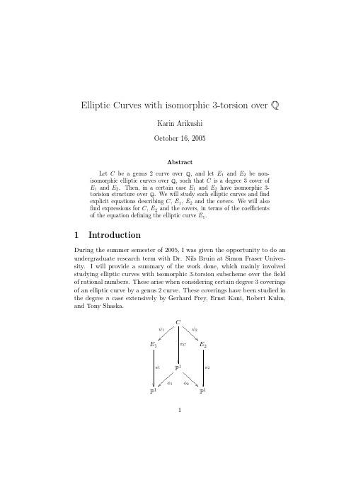
Elliptic Curves with isomorphic 3-torsion over QKarin ArikushiOctober 16,2005AbstractLet C be a genus 2curve over Q ,and let E 1and E 2be non-isomorphic elliptic curves over Q ,such that C is a degree 3cover of E 1and E 2.Then,in a certain case E 1and E 2have isomorphic 3-torision structure over Q .We will study such elliptic curves and find explicit equations describing C ,E 1,E 2and the covers.We will also find expressions for C ,E 2and the covers,in terms of the coefficients of the equation defining the elliptic curve E 1.1IntroductionDuring the summer semester of 2005,I was given the opportunity to do an undergraduate research term with Dr.Nils Bruin at Simon Fraser Univer-sity.I will provide a summary of the work done,which mainly involved studying elliptic curves with isomorphic 3-torsion subscheme over the field of rational numbers.These arise when considering certain degree 3coverings of an elliptic curve by a genus 2curve.These coverings have been studied in the degree n case extensively by Gerhard Frey,Ernst Kani,Robert Kuhn,and Tony Shaska.C ψ1||||||||πC ψ2B B B B B B B B E 1π1E 2π2P 1φ1}}}}}}}}φ2A A A A A A A A P 1P 11Let C be a genus2curve and E1an elliptic curve such thatφ1:C→E1is a degree3covering.Ifπ1andπC are specific coverings of the projective line (which we define later),then there exists an induced coveringφ1such that the left half of the diagram above commutes.We call this induced covering the Frey-Kani cover.Whenψ1is“non-degenerate”,C covers another elliptic curve E2with degree3,and induces another Frey-Kani cover so that the whole diagram commutes.When this occurs,E1and E2have isomorphic 3-torsion structure over Q,(Frey and Kani,[2]).We begin by providing some basic definitions and results involving ellip-tic curves,genus2curves,and coverings.Then we give a summary of work done by the mentioned authors,but we will only consider the case when the covering is degree3.For the most part,we are concerned with which genus2curves can form covers of elliptic curves in this way,and what the expressions for the Frey-Kani coverings and elliptic curves are.Finally,we finish with the results of our investigations.In their study of coverings of elliptic curves,the authors we mentioned worked mostly over an algebraically closedfield,such as C.We were able to find explicit equations for the elliptic curves E1and E2over Q.Also,given an elliptic curve E1over Q,we found explicit relations definingφ1:C→E1 in terms of the coefficients of E1,and found that the parameters for our genus2curve C are given by a genus zero curve,which has a rational point. 2PreliminariesWe begin with a discussion of elliptic curves and describe some of their basic properties.Definition1.An elliptic curve E over afield K is a nonsingular cubic curve in two variables,f(x,y)=0,together with a K-rational point.When char(K)=2,3we can write E in short Weierstrass form asE:y2=x3+ax+b where a,b∈K.The set of points(x0,y0)∈K×K that satisfy f(x0,y0)=0are the points on E over K,and is denoted E(K).Although we will not go into the details here,it is possible to define an “addition”operation on the points of an elliptic curve.Under this addition operation,the set of points forms a group,where the identity O,is usually taken to be the point at infinity.We are interested in the set of3-torsion points;the points P such that P+P+P=O.2Definition2.The setE(K)[n]={P∈E(K):nP=O}is the n-torsion group of E over K.Lemma1.For any elliptic curve E over an algebraically closedfield K,E(K)[n]∼=Z/n×Z/n.Lemma2.For any elliptic curve E over Q,E(Q)[3] Z/3×Z/3.Definition3.Two elliptic curves,E1and E2are isomorphic if there exists a birational regular map between E1and E2.Definition4.Let E1and E2be elliptic curves defined over Q.If there exists a birational mapΦ:E1[3](Q)→E2[3](Q),defined over Q that is a group homomorphism,we say that E1and E2have isomorphic3-torsion structure over Q.Over an algebraically closedfield,we canfind an isomorphism between the3-torsion groups of any pair of elliptic curves because we know what the group must be.However,over Q it is not generally true that two noniso-morphic elliptic curves will have isormorphic3-torsion groups.Keeping in mind how the group law works,it is easy to characterize the 2-and3-torsion points.For any elliptic curve E:f(x,y)=0,E(K)[2]is the set of points such that f(x0,0)=0and the identity.These are the points that are inverses of themselves under the group law.E(K)[3]is the set of inflection points,which occur in pairs above and below the x-axis,and the identity.This observation allows us tofind a degree four polynomial,whose roots are the x-coordinates of the non-zero 3-torsion points.If E:y2=x3+ax+b then,d2y dx =3x4+6ax2+12bx−a24y.Therefore,the eight inflection points on E are(x1,±y1),...,(x4,±y4),where the x i are roots of the numerator above,and the y i satisfy f(x i,y i)=0.As a subvariety of E,E(K)[3]is given by E∩Hessian(E).Note that E is a cubic,3so we will not see all8inflection points unless we are in an algebraically closedfield such as C or Q.Now that we know a little bit about elliptic curves,we should describe what genus2curves are like and what coverings are.For the purposes of this discussion,we can think of a genus2curve as given by a sextic in two variables,since any genus2curve can be written in the formC:y2=a6x6+···+a1x+a0.Definition 5.Let f:R→S be a non-constant rational map between curves.Then,f is a covering of S by R.Definition6.Given a covering f:R→S,thefibre of a point p∈S is{f−1(p)},and the degree of f,deg(f),is the maximum cardinality of allfibres over an algebraically closedfield.Definition7.Ramification points of a covering f:R→S are thefinite set of points p∈S such that|{f−1(p)}|<deg(f),over an algebraically closedfield.If p∈S and P∈{f−1(p)},then the number of branches going through P is the ramificaton index of P,denoted e f(p).We’ll give an example of a ramified covering of degree2.Example1.Let C:y2=w(x−w1)(x−w2)···(x−w6)be a genus2curve over an algebraically closedfield.Then,π:C→P1(x,y)→xis a degree2covering,with ramification points w1,...,w6.Each P i=(w i,0) lying above w i has ramification index2.The following result gives us a nice way to determine what the config-uration of ramification points for a cover might look like.We will use it extensively to determine expressions for the induced Frey-Kani coverings given in the next section.4Theorem 3.Riemann-HurwitzLet f :R →S be a covering.Then2(g (R )−1)=2deg(f )(g (S )−1)+p ∈R (e f (p )−1)where g (S )and g (T )denote the genus of S and T respectively.We’ve defined all the necessary objects to begin our discussion of how to construct elliptic curves with isomorphic 3-torsion structure of Q .3The constructionIn this section,we summarize the work pertaining to degree 3coverings of elliptic curves done by the authors mentioned in the introduction.The intention is to outline how the genus 2curves that form degree 3covers are characterized,how expressions for the Frey-Kani covers are determined,and when we have a second elliptic curve covered by the same genus 2curve.C ψ1||||||||πC AA A A A A A A E 1π1A A A A A A A A P 1φ1}}}}}}}P 1Let us start by defining the maps we want to study above.Definition 8.Let ψ1:C →E 1be a covering where,C :y 2=w (x −w 1)(x −w 2)···(x −w 6),where w i ∈QE 1:v 21=f 1(u 1)such that all coefficients are in Q .The maps πC :C →P 1,π1:E 1→P 1to the projective lines areπC (x,y )=x,π1(u 1,v 1)=u 1.These covers are all degree 2so we know by applying the Riemann-Hurwitz formula that πC has six ramification points,W ={w 1,...,w 6}above P 1,and π1has four,{q 1,...,q 4},which are precisely the points in5E 1(Q )[2].All these points have ramification index 2,but more importantly there exists an induced covering φ1(the Frey-Kani cover),such that the diagram above commutes.(See [2]).We are interested in φ1because a map between two projective lines is easier to work with than a map between two curves,ψ1.If ψ1:C →E 1is a degree 3cover,then Riemann-Hurwitz dictates thatP ∈C(e ψ1(P )−1)=2,so that ψ1is ramified above two points,each with ramification index 2(the non-degenerate case),or ψ1is ramified above only one place,with ramification index 3(the degenerate case).We are interested in the first case,so we will assume that ψ1is non-degenerate.Ramification of the Frey-Kani covering occurs in a similar way (see [4],Theorem 3.1),so that if ψ1is non-degenerate,then φ1has four points of ram-ification index 2.When ψ2is degenerate,φ2has two points of ramification index 2,and one point of ramification index 3.C ψ1||||||||πC ψ2B B B B B B B B E 1π1E 2π2P 1φ1}}}}}}}}φ2A A A A A A A A P 1P 1In the degree 3case,ψ1is called a maximal covering (since it does not factor over a nontrivial isogeny).When ψ1is maximal,there exists a second covering ψ2:C →E 2of an elliptic curve such that deg(ψ2)=deg(ψ1)(Shaska,[4]).A nice fact is that once ψ1is fixed,ψ2is unique up to isomorphism of elliptic curves (Kuhn,[3]),and it has a corresponding Frey-Kani cover φ2.To determine explicit equations for φ1and φ2,we look at the relation between the configuration of ramification points.Recall that π1is ramified in four places q 1,...,q 4.In the non-degenerate case,φ1is also ramified at four places,three of which are the same as π1(see [4]).Let these places be q 1,q 2and q 3,and let u 1=0be the fourth ramification point of φ1(the one not ramified in π1),such that x =0above6u1=0has ramification index2,and x=∞has ramification index1. We can do this because the fourth ramification point is rational[3].These conditions,with the fact that deg(φ1)=3dictate thatφ1(x)=x2x3+ax2+bx+cwhere c=0and the denominator has no repeated roots.Then,C is given by an equation of the formy2=(x3+ax2+bx+c)(4cx3+b2x2+2bcx+c2). Moreover,since the two coveringsψ1andψ2behave in a symmetric manner, the denominator ofφ2is4cx3+b2x2+2bcx+c2(see Kuhn,[3]).The roots of this cubic are unramified points ofφ2above u2=∞.φ2is ramified above u2=0,so let x=d be the point above u2=0with ramification index2, and x=e the point with ramification index1so thatφ2=(x−d)2(x−e)4cx+b x+2bcx+c.This determines the scaling ofφ2,and Kuhn in[3]gives possible values for d and e,d=−3cband,e=3ac2−b2c9c2−4abc+b3.We will verify that the expressions given for d and e are correct,once we determine explicit equations defining our elliptic curves E1and E2.4Expressions for E1and E2If a genus2curve C covers two nonisomorphic elliptic curves,E1and E2, with isomorphic3-torsion structure over Q,then C must be given by an equation of the formy2=(x3+ax2+bx+c)(4cx3+b2x2+2bcx+c2).Also,the maps from the x-line to the u1-line,respectively u2-line are defined to beφ1:P1→P1x→x2x3+ax2+bx+cφ2:P1→P1x→(x−d)2(x−e)4cx3+b2x2+2bcx+c2 7where d =−3c b ,e =3ac 2−b 2c 9c 2−4abc +b 3.Given this information,we would like to find explicit equations for both E 1and E 2,and find expressions for their coordinates u 1,v 1,u 2,v 2in terms of x and y .An expression for E 1is given by taking the discriminant of an expression involving φ1(x ).E 1:v 21=∆x (x 2−u 1(x 3+ax 2+bx +c ))u 1=(a 2b 2−27c 2+18abc −4a 3c −4b 3)u 31+(12a 2c −18bc −2ab 2)u 21+(b 2−12ac )u 1+4c.We already have u 1=φ1(x )and we obtain an expression for v 1by substi-tuting φ1(x )into the right-hand side above.After some basic manipulation we obtain v 1=y (x 3−bx −2c )(x 3+ax 2+bx +c )2Obtaining an expression for E 2is done in a similar manner,but we must take the correct twist of the curve.Again,we have u 2=φ2(x )and˜E 2:˜v 22=∆x ((x −d )2(x −e )−u 2(4cx 3+b 2x 2+2bcx +c 2))u 2=−16b 8c 4(27c 2−b 3)(9c 2−4abc +b 3)4u 32−16b 6c 4(27c 2−b 3)(9c 2−4abc +b 3)3(54ac 2+ab 3−27b 2c )u 22−16b 4c 4(27c 2−b 3)(9c 2−4abc +b 3)2(729a 2c 4+54a x b 3c 2−972ab 2c 3−18ab 5c +729bc 4+189b 4c 2+b 7)u 2+16b 2c 5(27c 2−b 3)(9c 2−4abc +b 3)(27c 2−9abc +2b 3)3.Substituting φ2(x )into the right-hand side,we obtain ˜v 2√s=y (b 3−27c 4)2((4abc −8c 2−b 3)x 3+(4ac 2−b 2c )x 2+bc 2x +c )(4cx 3+b 2x 2+2bcx +c 2)2wheres =16b 2c 4(9c 2−4abc +b 3).The correct twist of ˜E 2is obtained when v 2=˜v 2/√s ,so thatE 2:v 22=∆x ((x −d )2(x −e )−u 2(4cx 3+b 2x 2+2bcx +c 2))u 2.8Thus,we have obtained the correct expressions for E1and E2over Q. As mentioned,the authors we cite worked over C,so they did provide ex-pressions for E1and E2over C,but did not provide them over Q.5Verifying expressions forφ2In[3],Kuhn gives an expression forφ2:P1→P1,φ2(x)=(x−d)2(x−e)4cx3+b2x2+2bcx+c2,where d=−3cb,and e=3ac2−b2c9c2−4abc+b3.The configuration of ramification points dictates thatφ2must be in the above form,but we nevertheless spent some deriving the expressions for d and e correctly.To do this,we found∆x((x−d)2(x−e)−u2(4cx3+b2x2+2bcx+c2))u2,and made the substitution u2=φ2(x).The resulting expression should factor so that there is a cubic denominator,and a numerator that is the product of a constant in a,b,c,the factor x3+ax2+bx+c,and a square factor.We obtained a system of four equations from which we could derive the same expressions for d and e.There were other choices,but they would require an algebraic extension of Q.6Finding covers of a given elliptic curveGiven an elliptic curve E1,we were able tofind a genus2curve C,such that C is a non-degenerate degree3cover of E1.If E1is given by the equation˜v21=˜u31+g1˜u1+g0,then the goal is tofind the parameters a,b,c in the mapφ1:P1→P1x→x2x3+ax2+bx+c 9in terms of g1and g0,since C must be defined by an equation in the form y2=(x3+ax2+bx+c)(4cx3+b2x2+2bcx+c2).In the non-degenerate caseφ1is ramified in4places,above0,q1,q2and q3,which depend on a,b and c.If C is to cover E1,then the mapπ1:E1→P1(u1,v1)→u1should be ramified above q1,q2,q3and∞.Note that the ramification points here are the2-torsion points of E1.To accommodate this we shift and scale E1so that its2-torsion points lie at q1,q2,q3and∞by performing a change of variables,˜u1=Au1+B.In terms of the mapφ1,E1should be defined byv21=∆x(x2−u1(x3+ax2+bx+c))u1.Equating the right-hand side of the equation above to˜u1+g1˜u1+g0,and matching up the coefficients,we obtain a system of equations that a,b and c must satisfy.Solving the system using Maple,we see that a,b,c satisfy0=1147912560b3c8g31+5184b14a2g31+11664a2b14g20+972a4b13g20−288a4b13g31+4a6b12g31+27a6b12g20+17496a6b9c2g20−15058224a3b9c3g31−117074484a3b9c3g20+223205220b6c6g31−20995200ab10c3g31−4320a6b9c2g31−110539728ab10c3g20−2439314190ab7c5g20−259343208ab7g31c5+3779136a6b6c4g20+942244893a2b8c4g20+357128352a4b7c4g20+46924272a4b7c4g31−944784a5b8c3g31−4487724a5b8c3g20+156597948a2b8c4g31+2379456a2b11c2g31+354780a4b10c2g31+1738665a4b10c2g20+136048896a6c8g31−65664a3b12cg31+1119744a6b6c4g31−3507510600a3b6c5g20−576318240a3b6c5g31−68024448a5b5c5g31−510183360a5b5c5g20+1428513408a2b5c6g31+11823499368a2b5c6g20+1017532368a4b4c6g31+5892617808a4b4c6g20−155520ab13cg31−244944a3b12cg20−10206a5b11cg20+1944a5b11cg31+18738216a2b11c2g20+1793613375b6c6g20−1836660096a3c9g3110−24794911296a3c9g20+6198727824c10g31+4723920b12c2g20−1469664ab13cg20+1166400b12c2g31+159432300b9c4g20+15746400b9c4g31+46656b15g20−2219297616ab4c7g31+272097792a6b3c6g20+25194240a6b3c6g31−3095112384a3b3c7g31−23417416224a3b3c7g20−3673320192a5b2c7g20−612220032a5b2c7g31+30993639120a2b2c8g20+6887475360a2b2c8g31+1224440064a4bc8g31+16529940864a4bc8g20−8264970432abc9g31−12914016300ab4c7g20.The monster above is a weighted homogeneous equation in a,b and c, where the weights are1,2and3respectively,so we may assume that a=1. If we canfind(b0,c0)such that b0,c0∈Q,satisfying the equation then we have found a degree3cover of E1.Let h(b,c)equal the right-hand side above,with a=1.Then H:h=0 is a genus0curve with singular points(0,0),13,127,∞.Tofind a nonsingular point on H,fit a line though thefirst two singular points to obtain a third point on H,P=−4g3181g20,−4g31729g20.P is nonsingular for almost all values of g1and g0,except when(g1,g0)=(0,λ),(2λ2,−3λ2),whereλis a rational parameter.For these values of g1and g0,h becomes reducible.Notice that we have considerable choice in choosing a curve C that covers a given elliptic curve,E1.However,once the covering isfixed E2is uniquely determined,and we canfind an expression for it using the method outlined. References[1]Gerhard Frey,On elliptic curves with isomorphic torsion structures andcorresponding curves of genus2.[2]Gerhard Frey and Ernst Kani,Curves of genus2covering elliptic curvesand an arithmetical application,Prog.Math.89(1989),153–177(Eng-lish).11[3]Robert M.Kuhn,Curves of genus2with split Jacobian,Transactions ofthe American Mathematical Society307(1988),no.1,41–49(English).[4]Tony Shaska,Curves of genus2with(n,n)decomposable Jacobians,J.Symbolic Computation31(2001),no.5,603–617(English).[5],Genus2curves with(3,3)-split Jacobian and large automor-phism group,Lecture Notes in Computer Science,2369,Springer,2002, pp.205–218.[6],Genus2fields with degree3elliptic subfields,Forum Mathe-maticum16(2004),no.2,263–280(English).[7]Tony Shaska and Helmut V¨o lkein,Elliptic subfields and automorphismsof genus2functionfields,Algebra,Arithmetic and Geometry with Ap-plications,Springer,2004,pp.703–723(English).12。
AllYourCurvesandAllYourEdges(所有曲线和所有边缘)

UNIVERSITY OF CALIFORNIA, SAN DIEGOLove Your Curves and all Your EdgesA thesis submitted in partial satisfaction of the requirementsfor the degree Master of Fine ArtsinTheatre and Dance (Acting)byTesiana ElieCommittee in charge:Gregory Wallace, ChairUrsula MeyerCharles OatesManuel Rotenberg2015©Tesiana Elie, 2015 All rights reserved.The thesis of Tesiana Elie is approved and it is acceptable in quality and form for publication on microfilm and electronically:____________________________________ ____________________________________ ____________________________________ ____________________________________ChairUniversity of California, San Diego2015DEDICATIONI want to dedicate this to my mother. Without your teachings and discipline the advancement of my career and of my character would not be possible.I would also dedicate this to the fearsome foursome. Thank you for burning the midnight oil with me and forcing me to be a better artist everyday.Lastly I dedicate this to children who look like me, who come from less than ideal situations, and who have a dream. Your voice, and your lives matters.TABLE OF CONTENTSSignature Page (iii)Dedication (iv)Table of Contents (v)List of Supplemental Files (vi)Acknowledgements (vii)Abstract of the Thesis (viii)LIST OF SUPPLEMENTAL FILESFile 1. In the Crowding DarknessFile 2. She Stoops to ConquerFile 3. Burial of ThebesFile 4. Drums in the NightFile 5. HamlinFile 6. Tonight We ImproviseFile 7. In the Red and Brown WaterFile 8. VenusACKNOWLEDGEMENTSI want to give thanks first to God. I want to thank my faculty, Gregory Wallace, for passion and different viewpoints, Art Manke for specificity, Michael Rudko for thought, Eva Barnes for warmth and international peeks, Charlie Oats for treating me as family and reconnecting my body to my brain, Marco Barricelli for discoveries, Ursula Meyer for being tough and teaching me its ok not to smile when I’m hurt. To Linda Vickerman for reaching my falsetto and giving me keys to my melodies.Thank you Laura Manning, Michael Francis, Michael Fullerton, Doug Dutson, Laura Jimenez, Jim Carmody, Hedi Jafari, Mark Maltby, for always allowing me to burst into your office for no reason at all, and always welcoming me with open arms.Thank you to my class of divine leaders. Smoli Ollie, Tamms, Mad Dog, Kimbra, Lito, Romeo, Ler Bias. You guys inspire me, challenge me, and helped mold me into the woman I am today.Thank you to my extended mothers. Kyle Donnelly for feeding me mind, body, and soul, and to my mama bear Marybeth Ward who is my biggest supporter, the reason I came to grad school and my personal therapist.Thank you to my friends and family especially Daniella Dagrin, for being an excellent mother and educator. Thank you for being a great example for me to aspire to.ABSTRACT OF THE THESISLove Your Curves and all Your EdgesbyTesiana ElieMaster of Fine Arts in Theatre and Dance (Acting)University of California, San Diego, 2015Professor Gregory Wallace, ChairDuring this year I’ve formed many special relationships. The most intimate was being reintroduced to my skin and voice. I had the privilege to learn about Sarah Bartman. A woman whose beauty, women today are still trying to replicate. By learningthis woman I had the honor in learning about myself. Sarah was seen by all and heard to by none and sometimes as an actor I feel that way. But the beauty of Sarah was, she taught me how to use my voice when I felt the most hopeless. I had to learn how to be heard, while being proud of who I am. I know there is power in silence, but what I learned is that there is more power in being vulnerable.Nina Simone said, “It’s an artist’s duty to reflect the times in which we live.” Being here gave me the permission to call myself that. An artist. Where I come from names have power. So, if we as artist have power in our tongues, then can’t I also change the meaning of beauty? Can I be a reflection of the most powerful, diligent, and divine women I know, and not have a European standard looking back? What I’ve learned is that we have the authority to strip silent fears and public struggles of their bondage. So I’m not interested in the world’s standards I have my own. I would say this year was for reinforcing the curve of my hips and edge of my tongue.。
曲面曲线 curves and surfaces for CAGD
6B´e zier ApproximationB´e zier methods for curves and surfaces are popular,are commonly used in practical work, and are described here in detail.Two approaches to the design of a B´e zier curve are described,one using Bernstein polynomials and the other using the mediation operator. Both rectangular and triangular B´e zier surface patches are discussed,with examples.Historical NotesPierre Etienne B´e zier(pronounced“Bez-yea”or“bez-ee-ay”)was an applied math-ematician with the French car manufacturer Renault.In the early1960s,encouraged by his employer,he began searching for ways to automate the process of designing cars.His methods have been the basis of the modernfield of Computer Aided Geometric Design (CAGD),afield with practical applications in many areas.It is interesting to note that Paul de Faget de Casteljau,an applied mathematician with Citro¨e n,was thefirst,in1959,to develop the various B´e zier methods but—because of the secretiveness of his employer—never published it(except for two internal technical memos that were discovered in1975).This is why the entirefield is named after the second person,B´e zier,who developed it.B´e zier and de Casteljau did their work while working for car manufacturers.It is little known that Steven Anson Coons of MIT did most of his work on surfaces(around 1967)while a consultant for Ford.Another mathematician,William J.Gordon,has generalized the Coons surfaces,in1969,as part of his work for General Motors research labs.In addition,airplane designer James Ferguson also came up with the same ideas for the construction of curves and surfaces.It seems that car and airplane manufacturers have been very innovative in the CAGDfield.Detailed historical surveys of CAGD can be found in[Farin04]and[Schumaker81].176 6.B´e zier Approximation6.1The B´e zier CurveThe B´e zier curve is a parametric curve P(t)that is a polynomial function of the param-eter t.The degree of the polynomial depends on the number of points used to define the curve.The method employs control points and produces an approximating curve (note the title of this chapter).The curve does not pass through the interior points but is attracted by them(however,see Exercise6.7for an exception).It is as if the points exert a pull on the curve.Each point influences the direction of the curve by pulling it toward itself,and that influence is strongest when the curve gets nearest the point. Figure6.1shows some examples of cubic B´e zier curves.Such a curve is defined by four points and is a cubic polynomial.Notice that one has a cusp and another one has a loop.The fact that the curve does not pass through the points implies that the points are not“set in stone”and can be moved.This makes it easy to edit,modify and reshape the curve,which is one reason for its popularity.The curve can also be edited by adding new points,or deleting points.These techniques are discussed in Sections6.8and6.9, but they are cumbersome because the mathematical expression of the curve depends on the number of points,not just on the points themselves.P1Figure6.1:Four Plane Cubic and One Space B´e zier Curves With Their Control Points and Polygons.The control polygon of the B´e zier curve is the polygon obtained when the control points are connected,in their natural order,with straight segments.How does one go about deriving such a curve?We describe two approaches to the design—a weighted sum and a linear interpolation—and show that they are identical.6.1The B´e zier Curve 1776.1.1Pascal Triangle and the Binomial TheoremThe Pascal triangle and the binomial theorem are related because both employ the same numbers.The Pascal triangle is an infinite triangular matrix that’s built from the edges inside 11112113311464115101051.........We first fill the left and right edges with ones,then compute each interior element as the sum of the two elements directly above it.As can be expected,it is not hard to obtain an explicit expression for the general element of the Pascal triangle.We first number the rows from 0starting at the top,and the columns from 0starting on the left.A general element is denoted by i j .We then observe that the top two rows (corresponding to i =0,1)consist of 1’s and that every other row can be obtained as the sum of its predecessor and a shifted version of its predecessor.For example,1331+133114641This shows that the elements of the triangle satisfyi 0 = i i =1,i =0,1,..., i j = i −1j −1 + i −1j,i =2,3,...,j =1,2,...,(i −1).From this it is easy to derive the explicit expressioni j = i −1j −1 + i −1j=(i −1)!(j −1)!(i −j )!+(i −1)!j !(i −1−j )!=j (i −1)!j !(i −j )!+(i −j )(i −1)!j !(i −j )!=i !j !(i −j )!.Thus,the general element of the Pascal triangle is the well-known binomial coefficienti j =i !j !(i −j )!.178 6.B´e zier ApproximationThe binomial coefficient is one of Newton’s many contributions to mathematics. His binomial theorem states that(a+b)n=ni=0nia ib n−i.(6.1)This equation can be written in a symmetric way by denoting j=n−i.The result is(a+b)n=i+j=ni,j≥0(i+j)!i!j!a ib j,(6.2)from which we can easily guess the trinomial theorem(which is used in Section6.23)(a+b+c)n=i+j+k=ni,j,k≥0(i+j+k)!i!j!k!a ib jc k.(6.3)6.2The Bernstein Form of the B´e zier CurveThefirst approach to the B´e zier curve expresses it as a weighted sum of the points(with, of course,barycentric weights).Each control point is multiplied by a weight and the products are added.We denote the control points by P0,P1,...,P n(n is therefore defined as1less than the number of points)and the weights by B i.The expression ofweighted sum isP(t)=ni=0P i B i,0≤t≤1.The result,P(t),depends on the parameter t.Since the points are given by the user, they arefixed,so it is the weights that must depend on t.We therefore denote them by B i(t).How should B i(t)behave as a function of t?Wefirst examine B0(t),the weight associated with thefirst point P0.We want that point to affect the curve mostly at the beginning,i.e.,when t is close to0.Thus, as t grows toward1(i.e.,as the curve moves away from P0),B0(t)should drop down to 0.When B0(t)=0,thefirst point no longer influences the shape of the curve.Next,we turn to B1(t).This weight function should start small,should have a max-imum when the curve approaches the second point P1,and should then start dropping until it reaches zero.A natural question is:When(for what value of t)does the curve reach its closest approach to the second point?The answer is:It depends on the number of points.For three points(the case n=2),the B´e zier curve passes closest to the second point(the interior point)when t=0.5.For four points,the curve is nearest the second point when t=1/3.It is now clear that the weight functions must also depend on n and we denote them by B n,i(t).Hence,B3,1(t)should start at0,have a maximum at t=1/3,and go down to0from there.Figure6.2shows the desired behavior of B n,i(t)6.2The Bernstein Form of the B´e zier Curve179(*Just the base functions bern.Note how"pwr"handles0^0*)Clear[pwr,bern];pwr[x_,y_]:=If[x==0&&y==0,1,x^y];bern[n_,i_,t_]:=Binomial[n,i]pwr[t,i]pwr[1-t,n-i](*t^i x(1-t)^(n-i)*)Plot[Evaluate[Table[bern[5,i,t],{i,0,5}]],{t,0,1},DefaultFont->{"cmr10",10}];Figure6.2:The Bernstein Polynomials for n=2,3,4.for n=2,3,and4.Thefive different weights B4,i(t)have their maxima at t=0,1/4, 1/2,3/4,and1.The functions chosen by B´e zier(and also by de Casteljau)were derived by the Russian mathematician Serge˘ıNatanovich Bernshte˘ın in1912,as part of his work on approximation theory(see Chapter6of[Davis63]).They are known as the Bernstein polynomials and are defined byB n,i(t)=nit i(1−t)n−i,whereni=n!i!(n−i)!(6.4)are the binomial coefficients.These polynomials feature the desired behavior and have a few more useful properties that are discussed here.(In calculating the curve,we assume that the quantity00,which is normally undefined,equals1.)The B´e zier curve is now defined asP(t)=ni=0P i B n,i(t),where B n,i(t)=nit i(1−t)n−i and0≤t≤1.(6.5)Each control point(a pair or a triplet of coordinates)is multiplied by its weight,which is in the range[0,1].The weights act as blending functions that blend the contributions of the different points.Here is Mathematica code to calculate and plot the Bernstein polynomials and the B´e zier curve:(*Just the base functions bern.Note how"pwr"handles0^0*)Clear[pwr,bern,n,i,t]pwr[x_,y_]:=If[x==0&&y==0,1,x^y];bern[n_,i_,t_]:=Binomial[n,i]pwr[t,i]pwr[1-t,n-i](*t^i\[Times](1-t)^(n-i)*)Plot[Evaluate[Table[bern[5,i,t],{i,0,5}]],{t,0,1},DefaultFont->{"cmr10",10}]180 6.B´e zier ApproximationClear[i,t,pnts,pwr,bern,bzCurve,g1,g2];(*Cubic Bezier curve*)(*either read points from filepnts=ReadList["DataPoints",{Number,Number}];*)(*or enter them explicitly*)pnts={{0,0},{.7,1},{.3,1},{1,0}};(*4points for a cubic curve*)pwr[x_,y_]:=If[x==0&&y==0,1,x^y];bern[n_,i_,t_]:=Binomial[n,i]pwr[t,i]pwr[1-t,n-i]bzCurve[t_]:=Sum[pnts[[i+1]]bern[3,i,t],{i,0,3}]g1=ListPlot[pnts,Prolog->AbsolutePointSize[4],PlotRange->All,AspectRatio->Automatic,DisplayFunction->Identity]g2=ParametricPlot[bzCurve[t],{t,0,1},DisplayFunction->Identity]Show[g1,g2,DisplayFunction->$DisplayFunction]Next is similar code for a three-dimensional B´e zier curve.It was used to draw the space curve of Figure6.1.Clear[pnts,pwr,bern,bzCurve,g1,g2,g3];(*General3D Bezier curve*)pnts={{1,0,0},{0,-3,0.5},{-3,0,0.75},{0,3,1},{3,0,1.5},{0,-3,1.75},{-1,0,2}};n=Length[pnts]-1;pwr[x_,y_]:=If[x==0&&y==0,1,x^y];bern[n_,i_,t_]:=Binomial[n,i]pwr[t,i]pwr[1-t,n-i](*t^i x(1-t)^(n-i)*)bzCurve[t_]:=Sum[pnts[[i+1]]bern[n,i,t],{i,0,n}];g1=ParametricPlot3D[bzCurve[t],{t,0,1},Compiled->False,DisplayFunction->Identity];g2=Graphics3D[{AbsolutePointSize[2],Map[Point,pnts]}];g3=Graphics3D[{AbsoluteThickness[2],(*control polygon*)Table[Line[{pnts[[j]],pnts[[j+1]]}],{j,1,n}]}];g4=Graphics3D[{AbsoluteThickness[1.5],(*the coordinate axes*)Line[{{0,0,3},{0,0,0},{3,0,0},{0,0,0},{0,3,0}}]}];Show[g1,g2,g3,g4,AspectRatio->Automatic,PlotRange->All,DefaultFont->{"cmr10",10},Boxed->False,DisplayFunction->$DisplayFunction];Exercise6.1:Design a heart-shaped B´e zier curve based on nine control points.When B´e zier started searching for such functions in the early1960s,he set the following requirements[B´e zier86]:1.The functions should be such that the curve passes through thefirst and last control points.2.The tangent to the curve at the start point should be P1−P0,i.e.,the curve should start at point P0moving toward P1.A similar property should hold at the last point.3.The same requirement is generalized for higher derivatives of the curve at the two extreme endpoints.Hence,P tt(0)should depend only on thefirst point P0and its two neighbors P1and P2.In general,P(k)(0)should only depend on P0and its k neighbors P1through P k.This feature provides complete control over the continuity at the joints between separate B´e zier curve segments(Section6.5).4.The weight functions should be symmetric with respect to t and(1−t).This means that a reversal of the sequence of control points would not affect the shape of the curve.5.The weights should be barycentric,to guarantee that the shape of the curve is independent of the coordinate system.6.The entire curve lies within the convex hull of the set of control points.(See property8of Section6.4for a discussion of this point.)6.2The Bernstein Form of the B´e zier Curve 181The definition shown in Equation (6.5),using Bernstein polynomials as the weights,satisfies all these requirements.In particular,requirement 5is proved when Equa-tion (6.1)is written in the form [t +(1−t )]n =···(see Equation (6.12)if you cannot figure this out).Following are the explicit expressions of these polynomials for n =2,3,and 4.Example:For n =2(three control points),the weights areB 2,0(t )=(20)t 0(1−t )2−0=(1−t )2,B 2,1(t )=(21)t 1(1−t )2−1=2t (1−t ),B 2,2(t )=(22)t 2(1−t )2−2=t 2,and the curve isP (t )=(1−t )2P 0+2t (1−t )P 1+t 2P 2= (1−t )2,2t (1−t ),t 2 (P 0,P 1,P 2)T =(t 2,t,1)⎛⎝1−21−220100⎞⎠⎛⎝P 0P 1P 2⎞⎠.(6.6)This is the quadratic B´e zier curve.Exercise 6.2:Given three points P 1,P 2,and P 3,calculate the parabola that goes from P 1to P 3and whose start and end tangent vectors point in directions P 2−P 1and P 3−P 2,respectively.In the special case n =3,the four weight functions areB 3,0(t )=(30)t 0(1−t )3−0=(1−t )3,B 3,1(t )=(31)t 1(1−t )3−1=3t (1−t )2,B 3,2(t )=(32)t 2(1−t )3−2=3t 2(1−t ),B 3,3(t )=(33)t 3(1−t )3−3=t 3,and the curve isP (t )=(1−t )3P 0+3t (1−t )2P 1+3t 2(1−t )P 2+t 3P 3(6.7)= (1−t )3,3t (1−t )2,3t 2(1−t ),t 3 P 0,P 1,P 2,P 3 T = (1−3t +3t 2−t 3),(3t −6t 2+3t 3),(3t 2−3t 3),t 3 P 0,P 1,P 2,P 3 T =(t 3,t 2,t,1)⎛⎜⎝−13−313−630−33001000⎞⎟⎠⎛⎜⎝P 0P 1P 2P 3⎞⎟⎠.(6.8)It is clear that P (t )is a cubic polynomial in t .It is the cubic B´e zier curve.In general,the B´e zier curve for points P 0,P 1,...,P n is a polynomial of degree n .182 6.B´e zier ApproximationExercise6.3:Given the curve P(t)=(1+t+t2,t3),find its control points.Exercise6.4:The cubic curve of Equation(6.8)is drawn when the parameter t varies in the interval[0,1].Show how to substitute t with a new parameter u such that the curve will be drawn when−1≤u≤+1.Exercise6.5:Calculate the Bernstein polynomials for n=4.It can be proved by induction that the general,(n+1)-point B´e zier curve can be represented byP(t)=(t n,t n−1,...,t,1)N ⎛⎜⎜⎜⎜⎝P0P1...P n−1P n⎞⎟⎟⎟⎟⎠=T(t)·N·P,(6.9)whereN=⎛⎜⎜⎜⎜⎜⎜⎜⎝nnn(−1)nn1n−1n−1(−1)n−1···nnn−nn−n(−1)0nnn−1(−1)n−1n1n−1n−2(−1)n−2 0..... 0nn1(−1)1n1n−1(−1)0 0nn(−1)00 0⎞⎟⎟⎟⎟⎟⎟⎟⎠.(6.10)Matrix N is symmetric and its elements below the second diagonal are all zeros.Its determinant therefore equals(up to a sign)the product of the diagonal elements,which are all nonzero.A nonzero determinant implies a nonsingular matrix.Thus,matrix N always has an inverse.N can also be written as the product AB,whereA=⎛⎜⎜⎜⎜⎜⎜⎜⎝nn(−1)nn1n−1n−1(−1)n−1···nnn−nn−n(−1)0nn−1(−1)n−1n1n−1n−2(−1)n−2 0..... 0n1(−1)1n1n−1(−1)0 0n(−1)00 0⎞⎟⎟⎟⎟⎟⎟⎟⎠andB=⎛⎜⎜⎜⎝n0 0n1···0.........00···nn⎞⎟⎟⎟⎠.Figure6.3shows the B´e zier N matrices for n=1,2, (7)Exercise6.6:Calculate the B´e zier curve for the case n=1(two control points).What kind of a curve is it?6.2The Bernstein Form of the B´e zier Curve183N1=−1110,N2=⎛⎝1−21−220100⎞⎠,N3=⎛⎜⎝−13−313−630−33001000⎞⎟⎠,N4=⎛⎜⎜⎜⎝1−46−41−412−12406−12600−4400010000⎞⎟⎟⎟⎠,N5=⎛⎜⎜⎜⎜⎜⎝−15−1010−515−2030−2050−1030−30100010−2010000−550000100000⎞⎟⎟⎟⎟⎟⎠,N6=⎛⎜⎜⎜⎜⎜⎜⎜⎝1−615−2015−61−630−6060−306015−6090−601500−2060−602000015−30150000−66000001000000⎞⎟⎟⎟⎟⎟⎟⎟⎠,N7=⎛⎜⎜⎜⎜⎜⎜⎜⎜⎜⎝−17−2135−3521−717−42105−140105−4270−21105−210210−105210035−140210−14035000−35105−10535000021−422100000−7700000010000000⎞⎟⎟⎟⎟⎟⎟⎟⎟⎟⎠. Figure6.3:The First Seven B´e zier Basis Matrices.184 6.B´e zier ApproximationExercise6.7:Generally,the B´e zier curve passes through thefirst and last control points,but not through the intermediate points.Consider the case of three points P0, P1,and P2on a straight line.Intuitively,it seems that the curve will be a straight line and would therefore pass through the interior point P1.Is that so?The B´e zier curve can also be represented in a very compact and elegant way as P(t)=(1−t+tE)n P0,where E is the shift operator defined by E P i=P i+1(i.e., applying E to point P i produces point P i+1).The definition of E implies E P0=P1, E2P0=P2,and E i P0=P i.The B´e zier curve can now be writtenP(t)=ni=0nit i(1−t)n−i P i=ni=0nit i(1−t)n−i E i P0=ni=0ni(tE)i(1−t)n−i P0=tE+(1−t)nP0,where the last step is an application of the binomial theorem,Equation(6.1).Example:For n=1,this representation amounts toP(t)=(1−t+tE)P0=P0(1−t)+P1t.For n=2,we getP(t)=(1−t+tE)2P0=(1−t+tE−t+t2−t2E+tE−t2E+t2E2)P0=P0(1−2t+t2)+P1(2t−2t2)+P2t2=P0(1+t)2+P12t(1−t)+P2t2.Given n+1control points P0through P n,we can represent the B´e zier curve forthe points by P(n)n (t),where the quantity P(j)i(t)is defined recursively byP(j)i (t)=(1−t)P(j−1)i−1(t)+t P(j−1)i(t),for j>0,P i,for j=0.(6.11)The following examples show how the definition above is used to generate the quantitiesP(j)i (t)and why P(n)n(t)is the degree-n curve:P(0)(t)=P0,P(0)1(t)=P1,P(0)2(t)=P2,...,P(0)n(t)=P n,P(1)1(t)=(1−t)P(0)(t)+t P(0)1(t)=(1−t)P0+t P1,P(2)2(t)=(1−t)P(1)1(t)+t P(1)2(t)=(1−t)(1−t)P0+t P1+t(1−t)P1+t P2=(1−t)2P0+2t(1−t)P1+t2P2,P(3)3(t)=(1−t)P(2)2(t)+t P(2)3(t)6.3Fast Calculation of the Curve185=(1−t ) (1−t )P (1)1(t )+t P (1)2(t ) +t (1−t )P (1)2(t )+t P (1)3(t )=(1−t )2P (1)1(t )+2t (1−t )P (1)2(t )+t 2P (1)3(t )=(1−t )2 (1−t )P 0+t P 1 +2t (1−t ) (1−t )P 1+t P 2 +t 2 (1−t )P 2+t P 3=(1−t )3P 0+3t (1−t )2P 1+3t 2(1−t )P 2+t 3P 3.6.3Fast Calculation of the CurveCalculating the B´e zier curve is straightforward but slow.However,with a little thinking,it can be speeded up considerably,a feature that makes this curve very useful in practice.This section discusses three methods.Method 1:We notice the following:The calculation involves the binomials (ni )for i =0,1,...,n ,which,in turn,requirethe factorials 0!,1!,...,n !.The factorials can be precalculated once (each one from its predecessor)and stored in a table.They can then be used to calculate all the necessary binomials and those can also be stored in a table.The calculation involves terms of the form t i for i =0,1,...,n and for many t values in the interval [0,1].These can also be precalculated and stored in a two-dimensional table where they can be accessed later,using t and i as indexes.This has the advantage that the values of (1−t )n −i can be read from the same table (using 1−t and n −i as row and column indexes).The calculation now reduces to a sum where each term is a product of four quanti-ties,one control point and three numbers from tables.Instead of computingn i =0 ni t i (1−t )n −i P i ,we need to compute the simple sumni =0Table 1[i,n ]·Table 2[t,i ]·Table 2[1−t,n −i ]·P i .The parameter t is a real number that varies from 0to 1,so a practical implemen-tation of this method should use an integer T related to t .For example,if we increment t in 100steps,then T should be the integer 100t .Method 2:Once n is known,each of the n +1Bernstein polynomials B n,i (t ),i =0,1,...,n ,can be precalculated for all the necessary values of t and stored in a table.The curve can now be calculated as the sumni =0Table[t,i ]P i ,186 6.B´e zier Approximationindicating that each point on the computed curve requires n +1table lookups,n +1multiplications,and n additions.Again,an integer index T should be used instead of t .Method 3:Use forward differences in combination with the Taylor series represen-tation,to speed up the calculation significantly.The B´e zier curve,which we denote by B (t ),is drawn pixel by pixel in a loop where t is incremented from 0to 1in fixed,small steps of ∆t .The principle of forward differences (Section 1.5.1)is to find a quantity dB such that B (t +∆t )=B (t )+dB for any value of t .If such a dB can be found,then it is enough to calculate B (0)(which,as we know,is simply P 0)and use forward differences to calculateB (0+∆t )=B (0)+dB ,B (2∆t )=B (∆t )+dB =B (0)+2dB ,and,in general,B (i ∆t )=B (i −1)∆t +dB =B (0)+i dB .The point is that dB should not depend on t .If dB turns out to depend on t ,then as we advance t from 0to 1,we would have to use different values of dB ,slowing down the calculations.The fastest way to calculate the curve is to precalculate dB before the loop starts and to repeatedly add this precalculated value to B (t )inside the loop.We calculate dB by using the Taylor series representation of the B´e zier curve.In general,the Taylor series representation of a function f (t )at a point f (t +∆t )is the infinite sumf (t +∆t )=f (t )+f (t )∆t +f (t )∆2t 2!+f (t )∆3t 3!+···.In order to avoid dealing with an infinite sum,we limit our discussion to cubic B´e zier curves.These are the most common B´e zier curves and are used by many popular graph-ics applications.They are defined by four control points and are given by Equations (6.7)and (6.8):B (t )=(1−t )3P 0+3t (1−t )2P 1+3t 2(1−t )P 2+t 3P 3=(t 3,t 2,t,1)⎛⎜⎝−13−313−630−33001000⎞⎟⎠⎛⎜⎝P 0P 1P 2P 3⎞⎟⎠.These curves are cubic polynomials in t ,implying that only their first three derivatives are nonzero.In order to simplify the calculation of their derivatives,we need to express these curves in the form B (t )=a t 3+b t 2+c t +d [Equation (3.1)].This is done byB (t )=(1−t )3P 0+3t (1−t )2P 1+3t 2(1−t )P 2+t 3P 3= 3(P 1−P 2)−P 0+P 3 t 3+ 3(P 0+P 2)−6P 1 t 2+3(P 1−P 0)t +P 0=a t 3+b t 2+c t +d ,6.3Fast Calculation of the Curve187 so a=3(P1−P2)−P0+P3,b=3(P0+P2)−6P1,c=3(P1−P0),and d=P0. These relations can also be expressed in matrix notation⎛⎜⎝abcd⎞⎟⎠=⎛⎜⎝−13−313−630−33001000⎞⎟⎠⎛⎜⎝P0P1P2P3⎞⎟⎠.The curve is now easy to differentiateB t(t)=3a t2+2b t+c,B tt(t)=6a t+2b,B ttt(t)=6a; and the Taylor series representation yieldsdB=B(t+∆t)−B(t)=B t(t)∆t+B tt(t)∆2t2+B ttt(t)∆3t6=3a t2∆t+2b t∆t+c∆t+3a t∆2t+b∆2t+a∆3t.This seems like a failure since the value obtained for dB is a function of t(it should be denoted by dB(t)instead of just dB)and is also slow to calculate.However,the original cubic curve B(t)is a degree-3polynomial in t,whereas dB(t)is only a degree-2 polynomial.This suggests a way out of our dilemma.We can try to express dB(t)by means of the Taylor series,similar to what we did with the original curve B(t).This should result in a forward difference ddB(t)that’s a polynomial of degree1in t.The quantity ddB(t)can,in turn,be represented by another Taylor series to produce a forward difference dddB that’s a degree-0polynomial,i.e.,a constant.Once we do that,we will end up with an algorithm of the formprecalculate certain quantities;B=P0;for t:=0to1step∆t doPlotPixel(B);B:=B+dB;dB:=dB+ddB;ddB:=ddB+dddB;endfor;The quantity ddB(t)is obtained bydB(t+∆t)=dB(t)+ddB(t)=dB(t)+dB t(t)∆t+dB(t)tt∆2t2,yieldingddB(t)=dB t(t)∆t+dB(t)tt∆2t2=(6a t∆t+2b∆t+3a∆2t)∆t+6a∆t∆2t2=6a t∆2t+2b∆2t+6a∆3t.188 6.B´e zier ApproximationFinally,the constant dddB is similarly obtained byddB (t +∆t )=ddB (t )+dddB =ddB (t )+ddB t (t )∆t,yielding dddB =ddB t (t )∆t =6a ∆3t .The four quantities involved in the calculation of the curve are thereforeB (t )=a t 3+b t 2+c t +d ,dB (t )=3a t 2∆t +2b t ∆t +c ∆t +3a t ∆2t +b ∆2t +a ∆3t,ddB (t )=6a t ∆2t +2b ∆2t +6a ∆3t,dddB =6a ∆3t.They all have to be calculated at t =0,as functions of the four control points P i ,before the loop starts:B (0)=d =P 0,dB (0)=c ∆t +b ∆2t +a ∆3t =3∆t (P 1−P 0)+∆2t 3(P 0+P 2)−6P 1 +∆3t 3(P 1−P 2)−P 0+P 3=3∆t (P 1−P 0)+3∆2t (P 0−2P 1+P 2)+∆3t 3(P 1−P 2)−P 0+P 3 ,ddB (0)=2b ∆2t +6a ∆3t =2∆2t 3(P 0+P 2)−6P 1 +6∆3t 3(P 1−P 2)−P 0+P 3 =6∆2t (P 0−2P 1+P 2)+6∆3t 3(P 1−P 2)−P 0+P 3 ,dddB =6a ∆3t =6∆3t 3(P 1−P 2)−P 0+P 3 .The above relations can be expressed in matrix notation as follows:⎛⎜⎝dddB ddB (0)dB (0)B (0)⎞⎟⎠=⎛⎜⎝6000620011100001⎞⎟⎠⎛⎜⎝∆3t 0000∆2t 0000∆t 00001⎞⎟⎠⎛⎜⎝a b cd ⎞⎟⎠=⎛⎜⎝6000620011100001⎞⎟⎠⎛⎜⎝∆3t 0000∆2t 0000∆t 00001⎞⎟⎠⎛⎜⎝−13−313−630−33001000⎞⎟⎠⎛⎜⎝P 0P 1P 2P 3⎞⎟⎠=⎛⎜⎝−6∆3t 18∆3t −18∆3t 6∆3t 6∆2t −6∆3t −12∆2t +18∆3t 6∆2t −18∆3t 6∆3t 3∆2t −∆3t −3∆t −6∆2t +3∆3t +3∆t 3∆2t −3∆3t∆3t 1000⎞⎟⎠⎛⎜⎝P 0P 1P 2P 3⎞⎟⎠6.3Fast Calculation of the Curve189=Q ⎛⎜⎝P0P1P2P3⎞⎟⎠,where Q is a4×4matrix that can be calculated once∆t is known.A detailed examination of the above expressions shows that the following quantities have to be precalculated:3∆t,3∆2t,∆3t,6∆2t,6∆3t,P0−2P1+P2,and3(P1−P2)−P0+P3.We therefore end up with the simple,fast algorithm shown in Figure6.4.For those interested in a quick test,the corresponding Mathematica code is also included.Q1:=3∆t;Q2:=Q1×∆t;//3∆2tQ3:=∆3t;Q4:=2Q2;//6∆2tQ5:=6Q3;//6∆3tQ6:=P0−2P1+P2;Q7:=3(P1−P2)−P0+P3;B:=P0;dB:=(P1−P0)Q1+Q6×Q2+Q7×Q3;ddB:=Q6×Q4+Q7×Q5;dddB:=Q7×Q5;for t:=0to1step∆t doPixel(B);B:=B+dB;dB:=dB+ddB;ddB:=ddB+dddB;endfor;n=3;Clear[q1,q2,q3,q4,q5,Q6,Q7,B,dB,ddB,dddB,p0,p1,p2,p3,tabl];p0={0,1};p1={5,.5};p2={0,.5};p3={0,1};(*Four points*)dt=.01;q1=3dt;q2=3dt^2;q3=dt^3;q4=2q2;q5=6q3;Q6=p0-2p1+p2;Q7=3(p1-p2)-p0+p3;B=p0;dB=(p1-p0)q1+Q6q2+Q7q3;(*space indicates*)ddB=Q6q4+Q7q5;dddB=Q7q5;(*multiplication*)tabl={};Do[{tabl=Append[tabl,B],B=B+dB,dB=dB+ddB,ddB=ddB+dddB},{t,0,1,dt}]; ListPlot[tabl];Figure6.4:A Fast B´e zier Curve Algorithm.Each point of the curve(i.e.,each pixel in the loop)is calculated by three additions and three assignments only.There are no multiplications and no table lookups.This is a very fast algorithm indeed!190 6.B´e zier Approximation6.4Properties of the CurveThe following useful properties are discussed in this section:1.The weights add up to 1(they are barycentric).This is easily shown from Newton’s binomial theorem (a +b )n = n i =0 n i a i b n −i :1= t +(1−t ) n =n i =0 n i t i (1−t )n −i =n i =0B n,i (t ).(6.12)2.The curve passes through the two endpoints P 0and P n .We assume that 00=1and observe that B n,0(0)= n 0 00(1−0)n −0=1·1·1n =1,which impliesP (0)=n i =0P i B n,i (0)=P 0B n,0(0)=P 0.Also,the relationB n,n (1)=n n 1n (1−1)(n −n )=1·1·00=1,impliesP (1)=ni =0P i B n,i (1)=P n B n,n (1)=P n .3.Another interesting property of the B´e zier curve is its symmetry with respect to the numbering of the control points.If we number the points P n ,P n −1,...,P 0,we end up with the same curve,except that it proceeds from right (point P 0)to left (point P n ).The Bernstein polynomials satisfy the identity B n,j (t )=B n,n −j (1−t ),which can be proved directly and which can be used to prove the symmetrynj =0P j B n,j (t )=n j =0P n −j B n,j (1−t ).4.The first derivative (the tangent vector)of the curve is straightforward to derive P t (t )=n i =0P i B n,i (t )=n 0P i (n i ) i t i −1(1−t )n −i +t i (n −i )(1−t )n −i −1(−1) =nP i (n i )i t i −1(1−t )n −i −n −1 0P i (n i )t i (n −i )(1−t )n −1−i (using the identity n (n−1i −1)=i (n i ),we get)。
浙江省杭州市2023-2024学年高三上学期11月期中教学质量检测英语试题
浙江省杭州市2023-2024学年高三上学期11月期中教学质量检测英语试题学校:___________姓名:___________班级:___________考号:___________一、阅读理解1.Who is this article mainly intended for?A.Students in all grades.B.Students in 6th or 8th grades.C.Parents of children in 6th or 8th grades.D.Parents of children in 7th to 9th grades. 2.What do we know about Ravenna?A.It deals with entry applications.B.It promotes school management.C.It is accessible the whole school year.D.It monitors the admissions process. 3.Which can be a possible date for applicants to submit teacher evaluations?A.August 30, 2023.B.January 26, 2024.C.February 3, 2024.D.March 30, 2024.In 1959, Handler changed how toy dolls were made when she introduced “Barbie” to the world. With her mature figure, Barbie was one of the first “grown-up” dolls to hit the retail market.Handler wanted to create a toy that was different from the baby dolls that dominated little girls’ toy boxes. She wanted a doll that girls could project their future dreams upon and allowed for limitless clothing and career choices. Inspired by paper dolls of the time, Handler, to much disagreement, made sure Barbie had the body of a grown woman.“My own philosophy of Barbie,” Handler wrote in her autobiography, “was that through the doll, the little girl could be anything she wanted to be. Barbie always represented the fact that a woman had choices.”There’s even a Barbie for cancer patients — Brave Barbie — a partnership between Mattel and CureSearch that sends a bald (光头的) Barbie to families affected by cancer. “Gifting my daughter a Barbie who suffered from cancer was tremendous,” Michelle, a cancer survivor said, “We would play with that Barbie together and I’d heartbreakingly watch her pretend to take the doll to the hospital for chemo (化疗), or place its long wig on top of itshead and tell the doll ‘It’s time to be beautiful again.’”Bald Barbie was super brave and went on awesome adventures after chemo. Sometimes she felt sick and needed to sleep, but would feel much better after a rest. Bald Barbie always beat the cancer and went on to live a long and happy life with her family. That Barbie became so much more than a plastic doll — she was a means of communication and a coping mechanism during an extremely distressing time for little families.4.Why did Handler create Barbie?A.To make a hit in the retail market.B.To appeal to girls with her diverse outfits.C.To do a project on women’s career choices.D.To inspire girls to make choices as they wish.5.How might Michelle feel when watching her daughter with Brave Barbie?A.Sad yet comforted.B.Envious yet proud.C.Overwhelmed and ashamed.D.Heartbroken and regretful.6.What does Brave Barbie mean to Michelle’s family?A.A reliable emotional support.B.A glue for broken relationships.C.An effective practical treatment.D.A secret medium of negotiation. 7.Where is the text probably taken from?A.A medical journal.B.A charity brochure.C.A financial report.D.A story collection.That dinosaurs ate the mammals (哺乳动物) that ran beneath their feet is not in doubt. Now an extraordinary fossil newly described in Scientific Reports, unearthed by a team led by Gang Han at Hainan V ocational University of Science and Technology in China, shows that sometimes the tables were turned.The fossil -dated to about 125 million years ago, during the Cretaceous period-was formed when a flow of boiling volcanic mud swallowed two animals seemingly locked in a life-and-death fight. The one on top is a mammal. This animal is a herbivorous species closely related to the Triceratops (三角恐龙). Animal interactions such as this are exceptionally cam e in the fossil record.One possibility is that the mammal was eating something already dead, other than hunting live prey. These days it is uncommon for small mammals to attack much larger animals. But it is not unheard of. And Dr. Han and his colleagues point out that thosemammals which eat dead bodies typically leave tooth marks all over the bones of the animals. The dinosaur’s remains show no such marks. There is also a chance the fossil could be a fake. More and more convincing fake s have emerged, as this one did -though Dr. Han and his colleagues argue that the complexly connected nature of the skeletons (骨骼) makes that unlikely, too.Assuming it is genuine, the discovery serves as a reminder that not all dinosaurs were enormous during the Cretaceous and not all mammals were tiny. From nose to tail, the dinosaur is just 1.2 meters long. The mammal is a bit under half a meter in length. Despite being half the size, the mammal has one paw firmly wrapped around one of its prey’s limbs, and another pulling on its jaw. It is biting down on the dinosaur’s chest, and has ripped off two of its ribs. Before they were interrupted, it seems that the mammal was winning. 8.Which idiom is closest in meaning to underlined part “the tables were turned” in paragraph 1?A.The fittest survives.B.The hunters become hunted.C.Fortune always favors the brave.D.The truth will always come to light. 9.Why does the author mention the “tooth mark” in paragraph 3?A.To prove the fossil was fake.B.To show the forming of the fossil.C.To illustrate the process of hunting.D.To suggest the dinosaur was hunted alive.10.What makes Dr. Han think the fossil is genuine?A.The size of the fossil.B.The absence of fake fossils.C.The complexity of the skeletons.D.The consistency of the opinions. 11.What is the function of the last paragraph?A.It offers a cause.B.It highlights a solution.C.It justifies the conclusion.D.It provides a new discovery.Philosophers have a bad reputation for expressing themselves in a dry and boring way. The ideals for most philosophical writing are precision, clarity, and the sort of conceptual analysis that leaves no hair un-split.There is nothing wrong with clarity, precision, and the like — but this isn’t the only way to do philosophy. Outside academic journals, abstract philosophical ideas are often expressed through literature, cinema, and song. There’s nothing that grabs attention like a good story,and there are some great philosophical stories that delight and engage, rather than putting the reader to sleep.One of the great things about this is that, unlike formal philosophy, which tries to be very clear, stories don’t wear their meanings on their sleeve — they require interpretation, and often express conflicting ideas for the reader to wrestle with.Consider what philosophers call the metaphysics (形而上学) of race — an area of philosophy that explorers the question of whether or not race is real. There are three main positions that you can take on these questions. You might think that a person’s race is written in their genes (a position known as “biological realism”). Or you might think of race as socially real, like days of the week or currencies (“social constructionism”). Finally, you might think that races are unreal — that they’re more like leprechauns (一种魔法精灵) than they are like Thursdays or dollars (“anti-realism”).A great example of a story with social constructionist taking on race is George Schuyler’s novel Black No More. In the book, a Black scientist named Crookman invents a procedure that makes Black people visually indistinguishable from Whites. Thousands of African Americans flock to Crookman’s Black No More clinics and pay him their hard-earned cash to undergo the procedure. White racists can no longer distinguish those people who are “really” White from those who merely appear to be White. In a final episode, Crookman discovers that new Whites are actually a whiter shade of pale than those who were born that way, which kicks off a trend of sunbathing to darken one’s skin-darkening it so as to look more While.Philosophically rich stories like this bring more technical works to life. They are stories to think with.12.What does the author think of philosophical stories?A.The meaning behind is very obvious.B.They am extremely precise and formal.C.They often cause conflicts among readers.D.They are engaging and inspire critical thinking.13.Which category might “Christmas” fall into according to paragraph 4?A.Social constructionism.B.Anti-realism.C.Biological realism.D.Literary realism.14.What is Black No More in paragraph 5 mainly about?A.Racial issues caused by skin colors.B.A society view on race and self-image.C.Black people accepted by the white society.D.The origin of sun bathing among white people.15.What is the best title of the text?A.Stories Made Easy B.Stories to Think withC.Positions in Philosophy D.Nature of Philosophical Writing二、七选五In a world that often feels fast-paced and restrained to routines, the desire for van (房车)From the freedom to explore new horizons to fostering a minimalist mindset, here are some captivating advantages of embracing van life.Liberation from MaterialismThe confined space of a van encourages a minimalist lifestyle, where experiences are valued over possessions. 17 With minimal monthly expenses, such as parking fees and fuel costs, van dwellers can allocate resources to experiences rather than high rent or house payments. This mobile living is supported by the degrowth movement, which believes that economies should focus on securing the minimal basic needs instead of consumption and consumerism.Exploration and FlexibilityThe ability to follow adventure wherever it takes you is one of the most amazing aspects of living in a van. You can choose to wake up at dawn over the ocean one day and find yourself in a forested mountainside the next. Living in a van frequently involves being close to the outdoors surrounded by the beauty of nature. 18Minimal Ecological Footprint19 They adopt solar panels and efficient water systems , further minimizing their impact on the environment. People who choose to live in mobile homes believe that eventually, global warming and extreme weather might bring an end to sedentary (定居的) living patterns.Through the open road, the beauty of nature, and the friendship of fellow adventurers,van life presents a unique avenue for enriching the human experience. 20 A.It’s thrilling to travel the world.B.Many van lifers tend to go green.C.Living in a van can often be more cost-effective.D.They’ll find a sense of freedom of constant exploration.E.The natural world becomes an essential part of your daily lifeF.Better yet, it offers a way to reconnect with the essence of living.G.The concept of van life offers benefits beyond just a change of scenery.三、完形填空Gang (团伙) tensions were rising at Southwood High School. Some community activists23.A.voice B.status C.effort D.presence 24.A.safe B.hardworking C.healthy D.equal 25.A.practiced B.started C.gathered D.prepared 26.A.check B.maintain C.sacrifice D.arrange 27.A.large B.wild C.entire D.local 28.A.confusion B.anger C.fright D.shock 29.A.tricked B.persuaded C.forced D.scared 30.A.never B.unexpectedly C.further D.dramatically 31.A.happy B.curious C.cautious D.innovative 32.A.yell at B.interact with C.make fun of D.look up to 33.A.change B.post C.replace D.criticize 34.A.debate B.theft C.fight D.instance. 35.A.practical B.extraordinary C.temporary D.preventive四、用单词的适当形式完成短文阅读下面短文,在空白处填入1个适当的单词或括号内单词的正确形式。
抵抗天赋的诱惑(中英文)
抵抗天赋的诱惑(记贝索斯在普林斯顿大学2010年学士毕业典礼上的演讲) 我一直相信每一个人都有自己的天赋,每一个人的存在都代表着宇宙空间中的一种唯一,然而令我经常都在深思的是,既然我们都是这样的独特,又为何偏偏要去模仿和畸变成拥有同类“基因”的人呢?为什么我们中的很多人都不愿意去追逐属于自己的理想,或者不能为此奋斗一生呢,抑或者一生都是在自欺欺人的辩解?在Randy的The Last Lecture中我深深的感受到了一个人追逐自己最初理想的意义会变得如此的伟大,充满的是一种人生最大的和最根本的价值。
一直在想这样的一个问题,当社会尚且艰难,生活尚且苦难的日子里都有如此多人在追逐属于自己梦想的时候;在一个生活舒适,物质条件优越的年代我们竟然不知所措的迷失掉自己的方向,找不到自己前行的路。
这是多么可悲和可笑的一种境况!我们,有了更高的天赋,有了更好的环境,却因为有更多的选择而抹杀了我们自己的梦...这确实让人觉得不可思议!我相信每个人都有自己最初的梦想,在这样的一个年代,在这样一个至少没有饥寒交迫的时代,我坚信追逐自己理想的人会获得生命尽头最高贵的礼物和人生最大的价值!记:在一个可以实现最初梦想的时代选择不可以的沉默必将是这个时代最损失的损失,也必将是生活在这个时代的人最遗憾的遗憾...附:抵抗天赋的诱惑(贝索斯在普林斯顿大学2010年学士毕业典礼上的演讲)中文译稿:在我还是一个孩子的时候,我的夏天总是在德州祖父母的农场中度过。
我帮忙修理风车,为牛接种疫苗,也做其它家务。
每天下午,我们都会看肥皂剧,尤其是《我们的岁月》。
我的祖父母参加了一个房车俱乐部,那是一群驾驶Airstream拖挂型房车的人们,他们结伴遍游美国和加拿大。
每隔几个夏天,我也会加入他们。
我们把房车挂在祖父的小汽车后面,然后加入300余名Airstream探险者们组成的浩荡队伍。
我爱我的祖父母,我崇敬他们,也真心期盼这些旅程。
那是一次我大概十岁时的旅行,我照例坐在后座的长椅上,祖父开着车,祖母坐在他旁边,吸着烟。
TraditionalChineseMedicine
TraditionalChineseMedicineTraditional Chinese MedicineTraditional Chinese Medicine (TCM) is one of the great herbal systems of the world, dating back to the 3rd century BC. Yet throughout its history it has continually developed in response to changing clinical conditions, and has been sustained by research into every aspect of usage. This process continues today with the development of modern medical diagnostic techniques and knowledge. Chinese herbal medicines are very safe when prescribed correctly by a properly trained practitioner. Over thousands of years, experienced doctors have compiled detailed information about the pharmacopoeia and placed great emphasis on the protection of the patient.Allergic type reactions are rare, and will cause no lasting damage if treatment is stopped as soon as undesired symptoms appear. The primary difference between Chinese and Western medicine can be described as Chinese treats the Yang and Western treats the Yin. Everything in the universe can be described in terms of Yin or Yang. This is one of the underlying philosophies of Traditional Chinese Medicine. When applied to medicine in general, Western medicine acts upon the Yin of the body, the substance of the body, the actual cells and chemicals. Traditional medicine works more on the energy that animates those cells.Functions & Diagnostic MethodsFunctionsChinese medicine can be utilized to treat allergies, arthritis pain, weight control, quitting smoking, back injury pain, musculoskeletal pain, fatigue and stress. Other illnesses and conditions that can be helped with Chinese medicine are digestive problems, menstrual problems, and urinary problems.Chinese doctors greatly emphasis on lifestyle management in order to prevent disease before it occurs. Chinese medicine recognizes that health is more than just the absence of disease and it has a unique capacity to maintain and enhance our capacity for well being and happiness.Four Diagnostic MethodBianque, who regarded as the god doctor in Chinese medicine, applied the comprehensive diagnostic techniques of traditional Chinese medicines, namely, the four diagnostic methods: observation, auscultation and olfaction,interrogation, and pulse-feeling and palpation."Observation" means looking at the appearance and tongue fur. "Auscultation and olfaction"refers to listening to the sound of the patient's speech and breath. "Interrogation" refers to asking about the patient's symptoms and "pulse-feeling and palpation" is just in the literal meaning that feel the pulse by fingers' touch.Chinese Medical ClassicsThe Yellow Emperor's Internal ClassicThe Yellow Emperor's Internal Classic, or Internal Classic for short, whose author is unknown, is the earliest medical classic in China.It includes two parts: Plain Question and Acupuncture Classic, each of which comprises 9 volumes. The 18 volumes originally consist of 162 articles, even though some of the chaptershave been lost with the lapse of time. In a question-and-answer format, Plain Question recounts the discussion between the Yellow Emperor and his royal physician Qi Bo. It mainly sets forth the basic theories of physiology and pathology of the human body. Acupuncture Classic dwells upon acupuncture and moxibustion, main and collateral channels as well as hygiene and health care.Internal Classic lays the foundation for the theoretical systems of traditional Chinese medicine, which has long guided the clinical practice of Chinese medicine and played an important role in China’s medical history. It has great significance both inside and outside China. Parts of the book have been translated into Japanese, English, German and French. Many treatises on Internal Classic have been published in Japan.Compendium of Materia Medica (Ben Cao Gang Mu)Recorded in the 1.9-milions-words, 52-chapters, and 16-volumes are 1.897 varieties of medicines grouped under 60 categories. All the recorded medicines were in actual application and have proved effective by the author's time. BesidesChinese herbal medicine, they include animals and minerals for medication. In addition, the book contains 11,096 prescriptions and 1,160 illustrations. Such enormous contents enable the book to be the greatest treatise of material medica in history.Compendium of Materia Medica is more than a masterpiece of pharmaceutics, as it has also contributed to the human knowledge of biology, mineralogy and chemistry.Compendium of Materia Medica spread to Japan in 1606, then to Korea and Vietnam, and later to Europe around the 16th and 17th centuries. The book is now available either in whole or in excerpts in Latin, French, German, English, Russian and other languages. The world famous scientist Charles Darwin once consulted the book for historical data on the formation of skin colors of gold fish to demonstrate the artificial selection process of animals and gave high comments on it.Prescriptions Worth a Thousand Pieces of Gold for EmergenciesBeiji Qianjin Yaofang (Prescriptions Worth a Thousand Pieces of Gold for Emergencies), also called Qianjin Fang (Precious Prescriptions for Emergencies) or Qianjin Yaofang, was edited by Sun Simiao in the year 652. As Sun Simiao said, "Human life is of paramount importance, more precious than a thousand pieces of gold; to save it with one prescription is to show your great virtue", thus, 'gold" is used in the name of the book.From the Tang Dynasty (618-907) to the modern time, Beiji Qianjin Yaofang has had more than40 versions at home and abroad, which are roughly divided into two categories.The book is in 30 volumes. Volume 1 is the pandect of medical science, including medical ethics, materia medica, pharmacy and so on; Volume 2-4 are on gynecopathy; Volume 5 on pediatrics;Volume 6 on diseases of the seven orifices; Volume 7-8 on dermatophytosis of all kinds; Volume 9-10 on febrile diseases caused by cold; Volume 11-20 on viscera diseases; Volume 21 on diabetes and similar diseases; Volume 22 on skin and external diseases; Volume 23 onhemorrhoid; Volume 24 on disintoxicating and various treatments; Volume 25 on techniques for emergencies; Volume 26-27 on dietetic therapy and cultivation of mental poise; Volume 28 on normal pulse; and Volumes 29-30 on acupuncture and moxibustion. There are totally 233 categories, containing more than 5,300 articles. It has set up the format for compilation of prescriptions.A systematic summing-up of the accomplishments in medical science was concluded in this book before the Tang Dynasty. Its sources are extensive and its contents are abundant, covering all clinical sectors and many aspects such as acupuncture and moxibustion, dietetic therapy, medicament, prevention, hygiene and so on. It is the first comprehensive monumental works of medical science in China, another conclusion of Chinese medicine after Treatise on Febrile Diseases Caused by Cold and Miscellaneous Diseases by Zhang Zhongjing, and is praised as the earliest encyclopedia of clinical medicine in the Chinese history.Well-known DoctorsBianqueBianque, whose surname was Qin and original given name was Yueren, was born in Bohai (now Renqiu County of Hebei Province) in the Spring and Autumn and Warring States Period (770-221BC). When he was a child, he learned skills of Chinese medicine from an old folk doctor, Mr. Changsang. He mastered Mr. Changsang's diagnosis method and treatment techniques and became the most famous doctor in his time, and was an outstanding representative of medical experts in the Pre-Qin Period (before 221BC). He could diagnose diseases accurately, cure patients miraculously and bring the dying back to life. As a result, people respected him as a legendary god doctor and simply called him Bianque.After Bianque became famous, he toured all the kingdoms to cure more diseases and relieve more people from suffering. His areas of treatment often changed due to different regions. In Handan, he heard that most patients were women, so he worked as a "Daixia Doctor" (doctor specializing in gynecology); when he passed by Luoyang, he saw that elders were highly revered there so he became a doctor mainly treating diseases of the old such as the trouble in the ear or the eye; when he reached Xianyang, he became a pediatrician for people of the Qin Kingdom regarded children as the most important. In his practice of diagnosis, he had already applied the comprehensive diagnostic techniques of traditional Chinese medicines, namely, the four diagnostic methods: observation, auscultation and olfaction, interrogation, and pulse-feeling and palpation. At that time, Bianque called those techniques "Wangse (observing the color of the patient), Tingsheng (listening to the voice), Xieying (drawing a primary conclusion of the symptoms) and Qiemai (feeling the pulse)". Bianque's ways of treatment varied,such as acupuncture, adhibition of medicine, operation, medicine taking and so on.Bianque had nine disciples in his life who contributed to hand down his high medical skills from generation to generation. Till the Han Dynasty (206BC-220AD), his well-preserved works included nine volumes of Internal Canon of Medicine, twelve volumes of External Canon of Medicine, and thirteen volumes of Bianque's Prescriptions Approved by First Yellow Emperor, etc. The extant medical book of the Han Dynasty, Canon of Medicine of Difficult Diseases, is a work compiled on the basis of Bianque's medical skill, especially his knowledge on pulse-taking.Bianque was memorized and respected by Chinese people forever. Many basic theories of the traditional Chinese medicine, which is still playing a great role in the health service of mankind, are closely originated from or related to Bianque.Hua TuoHua Tuo, with a style name Yuanhua, also called Fu, was born approximately at the beginning of the second century AD and died before the 13th year of the Jian'an reign (208). He was an outstanding and eminent medical scientist in the Eastern Han Dynasty (25-220), especially good at surgical operation using anesthesia.When Hua Tuo was young, he studied in Xuzhou City of Jiangsu Province . He was skilled in several branches of learning and famous for his eminent performance. But he declined the conscription of the court to work as an officer and kept practicing medicine among the common people for a long time and his footprints covered many places including present Anhui , Shandong , Jiangsu , Henan and other provinces. He was deeply respected and loved by common people. In his late years, he was summoned by Cao Cao, a prominent legislator during the Three Kingdoms Period (220-280), to Xuchang of Hannan Province to treat the latter's wind syndrome of the head. Unwilling to work as Cao Cao's private doctor, Hua Tuo found an excuse to ask for leave and return to his home. He refused several times to come back to Xuchang, which angered Cao Cao. Finally, Cao Cao found an excuse to kill him.Hua Tuo advocated cure illness through exercise. He insisted that physical exercise was the key to strengthening the body, and movement could promote blood circulation and speed up metastases. And he used the sport of five animals created by himself to cure illness.Li ShizhenLi Shizhen (1518-1593), whose style name was Dongbi, also called Binhushanren (Person of the Mountain by the Lake) in his late years. He was from Jizhou (now Jichun County of Hubei Province) of the Ming Dynasty (1368-1644). His grandfather was a doctor, and his father Li Yanwen was also a famous doctor in the local place.As a child, Li Shizhen began to read some medical classics systematically. When his father went out for patients, he often went together with him to assistant for treating diseases and copying prescriptions. However, doctors' social position was low at that period so Li Yanwen did not hope Li Shizhen to take medicine as his occupation and asked him to take imperial examinations. For the sake of imperial examinations, he took Li Shizhen to Gu Riyan, a successful candidate in the imperial examination. Gu Riyan had a large collection of books, so Li Shizhen had the chance to read many rare classics.At the age of 17, 20 and 23, Li Shizhen went to Wuchang to take the imperial exam at the provincial level, but failed every time. Hence, he gave up the imperial examination and determined to follow his father to learn medicine. He lucubrated at medical knowledge, spared no pains to take in the predecessors' experiences in medical treatment and was good at giving play to his own creativity. Coupled with his high sympathy for patients, he did not only show good curative leechcraft but also high medical ethics in his practice. He won high prestige just ina few years. Particularly, his curing of a weird disease of children called "worm addiction" in theRoyal Family of Chu made his reputation rise rapidly, and he was employed by the royal family as "fengcizheng"(an official title), in charge of affairs in the "liangyisuo" (Office of Good Doctors).Later, he was recommended to the “Hospital of Imperial Physicians” in Beijing to work as the "yuanpan" (chief doctor). However, he was not interested in it and resigned on the pretext of illness after working only for a little more than one year. In his medical practice, Li Shizhen found many mistakes, repetitions or omissions in medical books available, feeling it was a great problem that affected the health and life of patients. So he made a decision to compile a new comprehensive book specializing in medicines again. From the age of 34, he started this project. In addition to summing-up of predecessors' experiences and accomplishments, he learned extensively from medical farmers, woodmen, hunters, fishermen and other laboring people. On the other hand, he often went to deep mountains and fields to observe and collect all kinds of samples of plants, animals, minerals and so on. He cultivated medical herbs himself and tried them on his own body so as to get the right knowledge of the herbs.After 27 years of efforts, with reference to more than 800 kinds of literature and based on Jingshi Zhenglei Beiji Bencao (abook on materia medica) by Tang Shenwei in the Song Dynasty (960-1279), he completed his monumental work in pharmacy, Compendium of Materia Medica, in the sixth year (1578) of the Wanli reign of the Ming Dynasty (1368-1644) at the age of 60, after he did a great deal of collation and supplementation, added many of his own findings and views, and carried out three important revisions. Li Shizhen will never be forgotten by people for his great contribution to traditional Chinese medicine.。
地磁场漂移与倒转
GGALVANIC DISTORTIONThe electrical conductivity of Earth materials affects two physical processes:electromagnetic induction which is utilized with magneto-tellurics(MT)(q.v.),and electrical conduction.If electromagnetic induction in media which are heterogeneous with respect to their elec-trical conductivity is considered,then both processes take place simul-taneously:Due to Faraday’s law,a variational electric field is induced in the Earth,and due to the conductivity of the subsoil an electric cur-rent flows as a consequence of the electric field.The current compo-nent normal to boundaries within the heterogeneous structure passes these boundaries continously according tos1E1¼s2E2where the subscripts1and2indicate the boundary values of conductiv-ity and electric field in regions1and2,respectively.Therefore the amplitude and the direction of the electric field are changed in the vicinity of the boundaries(Figure G1).In electromagnetic induction studies,the totality of these changes in comparison with the electric field distribution in homogeneous media is referred to as galvanic distortion. The electrical conductivity of Earth materials spans13orders of mag-nitude(e.g.,dry crystalline rocks can have conductivities of less than 10–6S mÀ1,while ores can have conductivities exceeding106S mÀ1). Therefore,MT has a potential for producing well constrained mod-els of the Earth’s electrical conductivity structure,but almost all field studies are affected by the phenomenon of galvanic distortion, and sophisticated techniques have been developed for dealing with it(Simpson and Bahr,2005).Electric field amplitude changes and static shiftA change in an electric field amplitude causes a frequency-indepen-dent offset in apparent resistivity curves so that they plot parallel to their true level,but are scaled by a real factor.Because this shift can be regarded as spatial undersampling or“aliasing,”the scaling factor or static shift factor cannot be determined directly from MT data recorded at a single site.If MT data are interpreted via one-dimensional modeling without correcting for static shift,the depth to a conductive body will be shifted by the square root of the factor by which the apparent resistivities are shifted.Static shift corrections may be classified into three broad groups: 1.Short period corrections relying on active near-surface measurementssuch as transient electromagnetic sounding(TEM)(e.g.,Meju,1996).2.Averaging(statistical)techniques.As an example,electromagneticarray profiling is an adaptation of the magnetotelluric technique that involves sampling lateral variations in the electric field con-tinuously,and spatial low pass filtering can be used to suppress sta-tic shift effects(Torres-Verdin and Bostick,1992).3.Long period corrections relying on assumed deep structure(e.g.,a resistivity drop at the mid-mantle transition zones)or long-periodmagnetic transfer functions(Schmucker,1973).An equivalence relationship exists between the magnetotelluric impedance Z and Schmucker’s C-response:C¼Zi om0;which can be determined from the magnetic fields alone,thereby providing an inductive scale length that is independent of the dis-torted electric field.Magnetic transfer functions can,for example, be derived from the magnetic daily variation.The appropriate method for correcting static shift often depends on the target depth,because there can be a continuum of distortion at all scales.As an example,in complex three-dimensional environments near-surface correction techniques may be inadequate if the conductiv-ity of the mantle is considered,because electrical heterogeneity in the deep crust creates additional galvanic distortion at a larger-scale, which is not resolved with near-surface measurements(e.g.,Simpson and Bahr,2005).Changes in the direction of electric fields and mixing of polarizationsIn some target areas of the MT method the conductivity distribution is two-dimensional(e.g.,in the case of electrical anisotropy(q.v.))and the induction process can be described by two decoupled polarizations of the electromagnetic field(e.g.,Simpson and Bahr,2005).Then,the changes in the direction of electric fields that are associated with galvanic distortion can result in mixing of these two polarizations. The recovery of the undistorted electromagnetic field is referred to as magnetotelluric tensor decomposition(e.g.,Bahr,1988,Groom and Bailey,1989).Current channeling and the“magnetic”distortionIn the case of extreme conductivity contrasts the electrical current can be channeled in such way that it is surrounded by a magneticvariational field that has,opposite to the assumptions made in the geo-magnetic deep sounding(q.v.)method,no phase lag with respect to the electric field.The occurrence of such magnetic fields in field data has been shown by Zhang et al.(1993)and Ritter and Banks(1998).An example of a magnetotelluric tensor decomposition that includes mag-netic distortion has been presented by Chave and Smith(1994).Karsten BahrBibliographyBahr,K.,1988.Interpretation of the magnetotelluric impedance tensor: regional induction and local telluric distortion.Journal of Geophy-sics,62:119–127.Chave,A.D.,and Smith,J.T.,1994.On electric and magnetic galvanic distortion tensor decompositions.Journal of Geophysical Research,99:4669–4682.Groom,R.W.,and Bailey,R.C.,1989.Decomposition of the magneto-telluric impedance tensor in the presence of local three-dimensional galvanic distortion.Journal of Geophysical Research,94: 1913–1925.Meju,M.A.,1996.Joint inversion of TEM and distorted MT sound-ings:some effective practical considerations.Geophysics,61: 56–65.Ritter,P.,and Banks,R.J.,1998.Separation of local and regional information in distorted GDS response functions by hypothetical event analysis.Geophysical Journal International,135:923–942. Schmucker,U.,1973.Regional induction studies:a review of methods and results.Physics of the Earth and Planetary Interiors,7: 365–378.Simpson,F.,and Bahr,K.,2005.Practical Magnetotellurics.Cam-bridge:Cambridge University Press.Torres-Verdin,C.,and Bostick,F.X.,1992.Principles of special sur-face electric field filtering in magnetotellurics:electromagnetic array profiling(EMAP).Geophysics,57:603–622.Zhang,P.,Pedersen,L.B.,Mareschal,M.,and Chouteau,M.,1993.Channelling contribution to tipper vectors:a magnetic equivalent to electrical distortion.Geophysical Journal International,113: 693–700.Cross-referencesAnisotropy,ElectricalGeomagnetic Deep SoundingMagnetotelluricsMantle,Electrical Conductivity,Mineralogy GAUSS’DETERMINATION OF ABSOLUTE INTENSITYThe concept of magnetic intensity was known as early as1600in De Magnete(see Gilbert,William).The relative intensity of the geomag-netic field in different locations could be measured with some preci-sion from the rate of oscillation of a dip needle—a method used by Humboldt,Alexander von(q.v.)in South America in1798.But it was not until Gauss became interested in a universal system of units that the idea of measuring absolute intensity,in terms of units of mass, length,and time,was considered.It is now difficult to imagine how revolutionary was the idea that something as subtle as magnetism could be measured in such mundane units.On18February1832,Gauss,Carl Friedrich(q.v.)wrote to the German astronomer Olbers:“I occupy myself now with the Earth’s magnetism,particularly with an absolute determination of its intensity.Friend Weber”(Wilhelm Weber,Professor of Physics at the University of Göttingen)“conducts the experiments on my instructions.As, for example,a clear concept of velocity can be given only through statements on time and space,so in my opinion,the complete determination of the intensity of the Earth’s magnetism requires to specify(1)a weight¼p,(2)a length¼r,and then the Earth’s magnetism can be expressed byffiffiffiffiffiffiffip=rp.”After minor adjustment to the units,the experiment was completed in May1832,when the horizontal intensity(H)at Göttingen was found to be1.7820mg1/2mm–1/2s–1(17820nT).The experimentThe experiment was in two parts.In the vibration experiment(Figure G2) magnet A was set oscillating in a horizontal plane by deflecting it from magnetic north.The period of oscillations was determined at different small amplitudes,and from these the period t0of infinite-simal oscillations was deduced.This gave a measure of MH,where M denotes the magnetic moment of magnet A:MH¼4p2I=t20The moment of inertia,I,of the oscillating part is difficult to deter-mine directly,so Gauss used the ingenious idea of conductingtheFigure G2The vibration experiment.Magnet A is suspended from a silk fiber F It is set swinging horizontally and the period of an oscillation is obtained by timing an integral number of swings with clock C,using telescope T to observe the scale S reflected in mirror M.The moment of inertia of the oscillating part can be changed by a known amount by hanging weights W from the rodR. 278GAUSS’DETERMINATION OF ABSOLUTE INTENSITYexperiment for I and then I þD I ,where D I is a known increment obtained by hanging weights at a known distance from the suspension.From several measures of t 0with different values of D I ,I was deter-mined by the method of least squares (another of Gauss ’s original methods).In the deflection experiment,magnet A was removed from the suspension and replaced with magnet B.The ratio M /H was measured by the deflection of magnet B from magnetic north,y ,produced by magnet A when placed in the same horizontal plane as B at distance d magnetic east (or west)of the suspension (Figure G3).This required knowledge of the magnetic intensity due to a bar magnet.Gauss deduced that the intensity at distance d on the axis of a dipole is inversely proportional to d 3,but that just one additional term is required to allow for the finite length of the magnet,giving 2M (1þk/d 2)/d 3,where k denotes a small constant.ThenM =H ¼1=2d 3ð1Àk =d 2Þtan y :The value of k was determined,again by the method of least squares,from the results of a number of measures of y at different d .From MH and M /H both M and,as required by Gauss,H could readily be deduced.Present methodsWith remarkably little modification,Gauss ’s experiment was devel-oped into the Kew magnetometer,which remained the standard means of determining absolute H until electrical methods were introduced in the 1920s.At some observatories,Kew magnetometers were still in use in the 1980s.Nowadays absolute intensity can be measured in sec-onds with a proton magnetometer and without the considerable time and experimental skill required by Gauss ’s method.Stuart R.C.MalinBibliographyGauss,C.F.,1833.Intensitas vis magneticae terrestris ad mensuram absolutam revocata.Göttingen,Germany.Malin,S.R.C.,1982.Sesquicentenary of Gauss ’s first measurement of the absolute value of magnetic intensity.Philosophical Transac-tions of the Royal Society of London ,A 306:5–8.Malin,S.R.C.,and Barraclough,D.R.,1982.150th anniversary of Gauss ’s first absolute magnetic measurement.Nature ,297:285.Cross-referencesGauss,Carl Friedrich (1777–1855)Geomagnetism,History of Gilbert,William (1544–1603)Humboldt,Alexander von (1759–1859)Instrumentation,History ofGAUSS,CARL FRIEDRICH (1777–1855)Amongst the 19th century scientists working in the field of geomag-netism,Carl Friedrich Gauss was certainly one of the most outstanding contributors,who also made very fundamental contributions to the fields of mathematics,astronomy,and geodetics.Born in April 30,1777in Braunschweig (Germany)as the son of a gardener,street butcher,and mason Johann Friderich Carl,as he was named in the certificate of baptism,already in primary school at the age of nine perplexed his teacher J.G.Büttner by his innovative way to sum up the numbers from 1to ter Gauss used to claim that he learned manipulating numbers earlier than being able to speak.In 1788,Gauss became a pupil at the Catharineum in Braunschweig,where M.C.Bartels (1769–1836)recognized his outstanding mathematical abilities and introduced Gauss to more advanced problems of mathe-matics.Gauss proved to be an exceptional pupil catching the attention of Duke Carl Wilhelm Ferdinand of Braunschweig who provided Gauss with the necessary financial support to attend the Collegium Carolinum (now the Technical University of Braunschweig)from 1792to 1795.From 1795to 1798Gauss studied at the University of Göttingen,where his number theoretical studies allowed him to prove in 1796,that the regular 17-gon can be constructed using a pair of compasses and a ruler only.In 1799,he received his doctors degree from the University of Helmstedt (close to Braunschweig;closed 1809by Napoleon)without any oral examination and in absentia .His mentor in Helmstedt was J.F.Pfaff (1765–1825).The thesis submitted was a complete proof of the fundamental theorem of algebra.His studies on number theory published in Latin language as Disquitiones arithi-meticae in 1801made Carl Friedrich Gauss immediately one of the leading mathematicians in Europe.Gauss also made further pioneering contributions to complex number theory,elliptical functions,function theory,and noneuclidian geometry.Many of his thoughts have not been published in regular books but can be read in his more than 7000letters to friends and colleagues.But Gauss was not only interested in mathematics.On January 1,1801the Italian astronomer G.Piazzi (1746–1820)for the first time detected the asteroid Ceres,but lost him again a couple of weeks later.Based on completely new numerical methods,Gauss determined the orbit of Ceres in November 1801,which allowed F.X.von Zach (1754–1832)to redetect Ceres on December 7,1801.This prediction made Gauss famous next to his mathematical findings.In 1805,Gauss got married to Johanna Osthoff (1780–1809),who gave birth to two sons,Joseph and Louis,and a daughter,Wilhelmina.In 1810,Gauss married his second wife,Minna Waldeck (1788–1815).They had three more children together,Eugen,Wilhelm,and Therese.Eugen Gauss later became the founder and first president of the First National Bank of St.Charles,Missouri.Carl Friedrich Gauss ’interest in the Earth magnetic field is evident in a letter to his friend Wilhelm Olbers (1781–1862)as early as 1803,when he told Olbers that geomagnetism is a field where still many mathematical studies can be done.He became more engaged in geo-magnetism after a meeting with A.von Humboldt (1769–1859)and W.E.Weber (1804–1891)in Berlin in 1828where von Humboldt pointed out to Gauss the large number of unsolved problems in geo-magnetism.When Weber became a professor of physics at the Univer-sity of Göttingen in 1831,one of the most productive periods intheFigure G3The deflection experiment.Suspended magnet B is deflected from magnetic north by placing magnet A east or west (magnetic)of it at a known distance d .The angle of deflection y is measured by using telescope T to observe the scale S reflected in mirror M.GAUSS,CARL FRIEDRICH (1777–1855)279field of geomagnetism started.In1832,Gauss and Weber introduced the well-known Gauss system according to which the magnetic field unit was based on the centimeter,the gram,and the second.The Mag-netic Observatory of Göttingen was finished in1833and its construc-tion became the prototype for many other observatories all over Europe.Gauss and Weber furthermore developed and improved instru-ments to measure the magnetic field,such as the unifilar and bifilar magnetometer.Inspired by A.von Humboldt,Gauss and Weber realized that mag-netic field measurements need to be done globally with standardized instruments and at agreed times.This led to the foundation of the Göttinger Magnetische Verein in1836,an organization without any for-mal structure,only devoted to organize magnetic field measurements all over the world.The results of this organization have been published in six volumes as the Resultate aus den Beobachtungen des Magnetischen Vereins.The issue of1838contains the pioneering work Allgemeine Theorie des Erdmagnetismus where Gauss introduced the concept of the spherical harmonic analysis and applied this new tool to magnetic field measurements.His general theory of geomagnetism also allowed to separate the magnetic field into its externally and its internally caused parts.As the external contributions are nowadays interpreted as current systems in the ionosphere and magnetosphere Gauss can also be named the founder of magnetospheric research.Publication of the Resultate ceased in1843.W.E.Weber together with such eminent professors of the University of Göttingen as Jacob Grimm(1785–1863)and Wilhelm Grimm(1786–1859)had formed the political group Göttingen Seven protesting against constitutional violations of King Ernst August of Hannover.As a consequence of these political activities,Weber and his colleagues were dismissed. Though Gauss tried everything to bring back Weber in his position he did not succeed and Weber finally decided to accept a chair at the University of Leipzig in1843.This finished a most fruitful and remarkable cooperation between two of the most outstanding contribu-tors to geomagnetism in the19th century.Their heritage was not only the invention of the first telegraph station in1833,but especially the network of36globally operating magnetic observatories.In his later years Gauss considered to either enter the field of bota-nics or to learn another language.He decided for the language and started to study Russian,already being in his seventies.At that time he was the only person in Göttingen speaking that language fluently. Furthermore,he was asked by the Senate of the University of Göttingen to reorganize their widow’s pension system.This work made him one of the founders of insurance mathematics.In his final years Gauss became fascinated by the newly built railway lines and supported their development using the telegraph idea invented by Weber and himself.Carl Friedrich Gauss died on February23,1855as a most respected citizen of his town Göttingen.He was a real genius who was named Princeps mathematicorum already during his life time,but was also praised for his practical abilities.Karl-Heinz GlaßmeierBibliographyBiegel,G.,and K.Reich,Carl Friedrich Gauss,Braunschweig,2005. Bühler,W.,Gauss:A Biographical study,Berlin,1981.Hall,T.,Carl Friedrich Gauss:A Biography,Cambridge,MA,1970. Lamont,J.,Astronomie und Erdmagnetismus,Stuttgart,1851. Cross-referencesHumboldt,Alexander von(1759–1859)Magnetosphere of the Earth GELLIBRAND,HENRY(1597–1636)Henry Gellibrand was the eldest son of a physician,also Henry,and was born on17November1597in the parish of St.Botolph,Aldersgate,London.In1615,he became a commoner at Trinity Col-lege,Oxford,and obtained a BA in1619and an MA in1621.Aftertaking Holy Orders he became curate at Chiddingstone,Kent,butthe lectures of Sir Henry Savile inspired him to become a full-timemathematician.He settled in Oxford,where he became friends withHenry Briggs,famed for introducing logarithms to the base10.Itwas on Briggs’recommendation that,on the death of Edmund Gunter,Gellibrand succeeded him as Gresham Professor of Astronomy in1627—a post he held until his death from a fever on16February1636.He was buried at St.Peter the Poor,Broad Street,London(now demolished).Gellibrand’s principal publications were concerned with mathe-matics(notably the completion of Briggs’Trigonometrica Britannicaafter Briggs died in1630)and navigation.But he is included herebecause he is credited with the discovery of geomagnetic secular var-iation.The events leading to this discovery are as follows(for furtherdetails see Malin and Bullard,1981).The sequence starts with an observation of magnetic declinationmade by William Borough,a merchant seaman who rose to“captaingeneral”on the Russian trade route before becoming comptroller ofthe Queen’s Navy.The magnetic observation(Borough,1581,1596)was made on16October1580at Limehouse,London,where heobserved the magnetic azimuth of the sun as it rose through sevenfixed altitudes in the morning and as it descended through the samealtitudes in the afternoon.The mean of the two azimuths for each alti-tude gives a measure of magnetic declination,D,the mean of which is11 190EÆ50rms.Despite the small scatter,the value could have beenbiased by site or compass errors.Some40years later,Edmund Gunter,distinguished mathematician,Gresham Professor of Astronomy and inventor of the slide rule,foundD to be“only6gr15m”(6 150E)“as I have sometimes found it oflate”(Gunter,1624,66).The exact date(ca.1622)and location(prob-ably Deptford)of the observation are not stated,but it alerted Gunterto the discrepancy with Borough’s measurement.To investigatefurther,Gunter“enquired after the place where Mr.Borough observed,and went to Limehouse with...a quadrant of three foot Semidiameter,and two Needles,the one above6inches,and the other10inches long ...towards the night the13of June1622,I made observation in sev-eral parts of the ground”(Gunter,1624,66).These observations,witha mean of5 560EÆ120rms,confirmed that D in1622was signifi-cantly less than had been measured by Borough in1580.But was thisan error in the earlier measure,or,unlikely as it then seemed,was Dchanging?Unfortunately Gunter died in1626,before making anyfurther measurements.When Gellibrand succeeded Gunter as Gresham Professor,allhe required to do to confirm a major scientific discovery was towait a few years and then repeat the Limehouse observation.Buthe chose instead to go to the site of Gunter’s earlier observationin Deptford,where,in June1633,Gellibrand found D to be“muchless than5 ”(Gellibrand,1635,16).He made a further measurement of D on the same site on June12,1634and“found it not much to exceed4 ”(Gellibrand,1635,7),the published data giving4 50 EÆ40rms.His observation of D at Paul’s Cray on July4,1634adds little,because it is a new site.On the strength of these observations,he announced his discovery of secular variation(Gellibrand,1635,7and 19),but the reader may decide how much of the credit should go to Gunter.Stuart R.C.Malin280GELLIBRAND,HENRY(1597–1636)BibliographyBorough,W.,1581.A Discourse of the Variation of the Compass,or Magnetical Needle.(Appendix to R.Norman The newe Attractive).London:Jhon Kyngston for Richard Ballard.Borough,W.,1596.A Discourse of the Variation of the Compass,or Magnetical Needle.(Appendix to R.Norman The newe Attractive).London:E Allde for Hugh Astley.Gellibrand,H.,1635.A Discourse Mathematical on the Variation of the Magneticall Needle.Together with its admirable Diminution lately discovered.London:William Jones.Gunter,E.,1624.The description and use of the sector,the crosse-staffe and other Instruments.First booke of the crosse-staffe.London:William Jones.Malin,S.R.C.,and Bullard,Sir Edward,1981.The direction of the Earth’s magnetic field at London,1570–1975.Philosophical Transactions of the Royal Society of London,A299:357–423. Smith,G.,Stephen,L.,and Lee,S.,1967.The Dictionary of National Biography.Oxford:University Press.Cross-referencesCompassGeomagnetic Secular VariationGeomagnetism,History ofGEOCENTRIC AXIAL DIPOLE HYPOTHESISThe time-averaged paleomagnetic fieldPaleomagnetic studies provide measurements of the direction of the ancient geomagnetic field on the geological timescale.Samples are generally collected at a number of sites,where each site is defined as a single point in time.In most cases the time relationship between the sites is not known,moreover when samples are collected from a stratigraphic sequence the time interval between the levels is also not known.In order to deal with such data,the concept of the time-averaged paleomagnetic field is used.Hospers(1954)first introduced the geocentric axial dipole hypothesis(GAD)as a means of defining this time-averaged field and as a method for the analysis of paleomag-netic results.The hypothesis states that the paleomagnetic field,when averaged over a sufficient time interval,will conform with the field expected from a geocentric axial dipole.Hospers presumed that a time interval of several thousand years would be sufficient for the purpose of averaging,but many studies now suggest that tens or hundreds of thousand years are generally required to produce a good time-average. The GAD model is a simple one(Figure G4)in which the geomag-netic and geographic axes and equators coincide.Thus at any point on the surface of the Earth,the time-averaged paleomagnetic latitude l is equal to the geographic latitude.If m is the magnetic moment of this time-averaged geocentric axial dipole and a is the radius of the Earth, the horizontal(H)and vertical(Z)components of the magnetic field at latitude l are given byH¼m0m cos l;Z¼2m0m sin l;(Eq.1)and the total field F is given byF¼ðH2þZ2Þ1=2¼m0m4p a2ð1þ3sin2lÞ1=2:(Eq.2)Since the tangent of the magnetic inclination I is Z/H,thentan I¼2tan l;(Eq.3)and by definition,the declination D is given byD¼0 :(Eq.4)The colatitude p(90 minus the latitude)can be obtained fromtan I¼2cot pð0p180 Þ:(Eq.5)The relationship given in Eq. (3) is fundamental to paleomagnetismand is a direct consequence of the GAD hypothesis.When applied toresults from different geologic periods,it enables the paleomagneticlatitude to be derived from the mean inclination.This relationshipbetween latitude and inclination is shown in Figure G5.Figure G5Variation of inclination with latitude for a geocentricdipole.GEOCENTRIC AXIAL DIPOLE HYPOTHESIS281Paleom a gnetic polesThe positio n where the time-averaged dipole axis cuts the surface of the Earth is called the paleomagnetic pole and is defined on the present latitude-longitude grid. Paleomagnetic poles make it possible to com-pare results from different observing localities, since such poles should represent the best estimate of the position of the geographic pole.These poles are the most useful parameter derived from the GAD hypothesis. If the paleomagnetic mean direction (D m , I m ) is known at some sampling locality S, with latitude and longitude (l s , f s ), the coordinates of the paleomagnetic pole P (l p , f p ) can be calculated from the following equations by reference to Figure G6.sin l p ¼ sin l s cos p þ cos l s sin p cos D m ðÀ90 l p þ90 Þ(Eq. 6)f p ¼ f s þ b ; when cos p sin l s sin l porf p ¼ f s þ 180 À b ; when cos p sin l s sin l p (Eq. 7)wheresin b ¼ sin p sin D m = cos l p : (Eq. 8)The paleocolatitude p is determined from Eq. (5). The paleomagnetic pole ( l p , f p ) calculated in this way implies that “sufficient ” time aver-aging has been carried out. What “sufficient ” time is defined as is a subject of much debate and it is always difficult to estimate the time covered by the rocks being sampled. Any instantaneous paleofield direction (representing only a single point in time) may also be con-verted to a pole position using Eqs. (7) and (8). In this case the pole is termed a virtual geomagnetic pole (VGP). A VGP can be regarded as the paleomagnetic analog of the geomagnetic poles of the present field. The paleomagnetic pole may then also be calculated by finding the average of many VGPs, corresponding to many paleodirections.Of course, given a paleomagnetic pole position with coordinates (l p , f p ), the expected mean direction of magnetization (D m , I m )at any site location (l s , f s ) may be also calculated (Figure G6). The paleocolatitude p is given bycos p ¼ sin l s sin l p þ cos l s cos l p cos ðf p À f s Þ; (Eq. 9)and the inclination I m may then be calculated from Eq. (5). The corre-sponding declination D m is given bycos D m ¼sin l p À sin l s cos pcos l s sin p; (Eq. 10)where0 D m 180 for 0 (f p – f s ) 180and180 < D m <360for 180 < (f p –f s ) < 360 .The declination is indeterminate (that is any value may be chosen)if the site and the pole position coincide. If l s ¼Æ90then D m is defined as being equal to f p , the longitude of the paleomagnetic pole.Te s ting the GAD hy p othesis Tim e scale 0– 5 MaOn the timescale 0 –5 Ma, little or no continental drift will have occurred, so it was originally thought that the observation that world-wide paleomagnetic poles for this time span plotted around the present geographic indicated support for the GAD hypothesis (Cox and Doell,1960; Irving, 1964; McElhinny, 1973). However, any set of axial mul-tipoles (g 01; g 02 ; g 03 , etc.) will also produce paleomagnetic poles that cen-ter around the geographic pole. Indeed, careful analysis of the paleomagnetic data in this time interval has enabled the determination of any second-order multipole terms in the time-averaged field (see below for more detailed discussion of these departures from the GAD hypothesis).The first important test of the GAD hypothesis for the interval 0 –5Ma was carried out by Opdyke and Henry (1969),who plotted the mean inclinations observed in deep-sea sediment cores as a function of latitude,showing that these observations conformed with the GAD hypothesis as predicted by Eq. (3) and plotted in Figure G5.Testing the axial nature of the time-averaged fieldOn the geological timescale it is observed that paleomagnetic poles for any geological period from a single continent or block are closely grouped indicating the dipole hypothesis is true at least to first-order.However,this observation by itself does not prove the axial nature of the dipole field.This can be tested through the use of paleoclimatic indicators (see McElhinny and McFadden,2000for a general discus-sion).Paleoclimatologists use a simple model based on the fact that the net solar flux reaching the surface of the Earth has a maximum at the equator and a minimum at the poles.The global temperature may thus be expected to have the same variation.The density distribu-tion of many climatic indicators (climatically sensitive sediments)at the present time shows a maximum at the equator and either a mini-mum at the poles or a high-latitude zone from which the indicator is absent (e.g.,coral reefs,evaporates,and carbonates).A less common distribution is that of glacial deposits and some deciduous trees,which have a maximum in polar and intermediate latitudes.It has been shown that the distributions of paleoclimatic indicators can be related to the present-day climatic zones that are roughly parallel with latitude.Irving (1956)first suggested that comparisons between paleomag-netic results and geological evidence of past climates could provide a test for the GAD hypothesis over geological time.The essential point regarding such a test is that both paleomagnetic and paleoclimatic data provide independent evidence of past latitudes,since the factors con-trolling climate are quite independent of the Earth ’s magnetic field.The most useful approach is to compile the paleolatitude values for a particular occurrence in the form of equal angle or equalareaFigure G6Calculation of the position P (l p ,f p )of thepaleomagnetic pole relative to the sampling site S (l s ,f s )with mean magnetic direction (D m ,I m ).282GEOCENTRIC AXIAL DIPOLE HYPOTHESIS。
- 1、下载文档前请自行甄别文档内容的完整性,平台不提供额外的编辑、内容补充、找答案等附加服务。
- 2、"仅部分预览"的文档,不可在线预览部分如存在完整性等问题,可反馈申请退款(可完整预览的文档不适用该条件!)。
- 3、如文档侵犯您的权益,请联系客服反馈,我们会尽快为您处理(人工客服工作时间:9:00-18:30)。
for all q . In particular this yields that A(q ) = q 1/2 − 1 if q is a square. Garcia and Stichtenoth [1], [3] proved that if q is a square, then A(q ) = q 1/2 − 1 can be achieved by an explicitly constructed tower of global function fields. In the case where q is not a square, no exact values of A(q ) are known, but lower bounds are available which complement the general upper bound (2). According to a result of Serre [16], [17] (see also [11]) based on class field towers, we have A(q ) ≥ c log q with an absolute constant cห้องสมุดไป่ตู้> 0. Zink [22] gave the best known lower bound for p3 : A(p3 ) ≥ 2(p2 − 1) . p+2 (4) (3)
8 8 = 0.4705 . . . and A(5) ≥ 11 = 0.7272 . . ., thus It is also shown in [19] that A(3) ≥ 17 improving the corresponding bounds given in [10]. In this paper we employ class field towers to improve aforementioned lower bounds for A(q ) and to compute A(p) for small primes p. We also give an alternative proof of Theorem 1.5 with an explicit and improved constant c. Finally, we present a lower bound for the l-rank of the S -divisor class group, similar to the corresponding result from [10]. More precisely, our results are as follows. By using the explicit construction of ray class fields of function fields via rank one Drinfeld modules we prove the following generalisation of Theorem 1.3.
25 August 1999
Abstract The number A(q ) is the upper limit of the ratio of the maximum number of points of a curve defined over Fq to the genus. By constructing class field towers with good parameters we present improvements of lower bounds of A(q ) for q an odd power of a prime.
3
(14)
Recently Temkine [19] extended Serre’s lower bound (3) to Theorem 1.5 There exists an effective constant c such that A(q r ) ≥ cr 2 log q log q . log r + log q (15)
1
Introduction
Given a finite field I Fq of q elements, by K/I Fq we mean a global function field K with full constant field I Fq , that is, with I Fq algebraically closed in K . A rational place of K is a place of K of degree 1. Write N (K ) for the number of rational places of K and g (K ) for the genus of K . According to the Weil-Serre bound (see [16], [17]) we have N (K ) ≤ q + 1 + g (K )⌊2q 1/2 ⌋, where ⌊t⌋ is the greatest integer not exceeding the real number t. Definition 1.1 For any prime power q and any integer g ≥ 0 put Nq (g ) = max N (K ), where the maximum is extended over all global function fields K of genus g with full constant field I Fq . In other words, Nq (g ) is the maximum number of I Fq -rational points that a smooth, projective, absolutely irreducible algebraic curve over I Fq of genus g can have. The following quantity was introduced by Ihara [7]. Definition 1.2 For any prime power q let A(q ) = lim supg→∞
Coverings of curves with asymptotically many rational points ∗
Wen-Ching W Li and Hiren Maharaj
arXiv:math/9908152v1 [math.NT] 28 Aug 1999
Department. of Mathematics Pennsylvania State University University Park, PA 16802-6401 wli@, maharaj@
(2) If q is even and Br (F ) ≥ 2(2N − 2)1/2 + 3, then A(q r ) ≥ (9)
The bounds (6) and (7) follow from the above theorem by considering the rational function field over Fq . Using this theorem, they also found improved lower bounds for A(q 3 ): Corollary 1.4 (1) If q is a power of an odd prime p and p does not divide ⌊2q 1/2 ⌋, then 2q + 4⌊q 1/2 ⌋ A(q ) ≥ . 3 + ⌈2(2q + 4⌊q 1/2 ⌋ + 1)1/2 ⌉
∗
(1)
Nq (g ) . g
Research supported in part by the NSF grants DMS96-22938 and DMS99-70651.
1
It follows from (1) that A(q ) ≤ ⌊2q 1/2 ⌋. Furthermore, Ihara [7] showed that A(q ) ≥ q 1/2 − 1 if q is a square. In the special cases q = p2 and q = p4 , this lower bound was also proved by Tsfasman, Vlˇ adut, and Zink [20]. Hereafter, p always denotes a prime number. Vlˇ adut and Drinfel’d [21] established the bound A(q ) ≤ q 1/2 − 1 (2)
If q ≥ 4 is even and m ≥ 3 is an odd integer, then A(q m ) ≥ (7)
As a consequence, they improved the Gilbert-Varshamov bound for sufficiently large composite nonsquare q on a certain interval. Furthermore in [10] they showed that 81 62 A(2) ≥ 317 = 0.2555 . . ., A(3) ≥ 163 = 0.3803 . . . and A(5) ≥ 2 = 0.666 . . .. 3 Denote the number of places of degree r in a function field F by Br (F ) or simply Br if there is no danger of confusion. Niederreiter and Xing further extended their bounds (6) and (7) to the following result in [11]. Theorem 1.3 Let F/Fq be a global function field with N ≥ 1 rational places. Let r ≥ 3 be an integer. Suppose that the ratio of class numbers h(F Fqr )/h(F ) is odd. (1) If q is odd and Br (F ) ≥ 2(2N − 1)1/2 + 3, then A(q r ) ≥ 2(N − 1) . 2g (F ) + ⌈2(2N − 1)1/2 ⌉ + 1 N −1 . g (F ) + ⌈2(2N − 2)1/2 ⌉ + 2 2 (8)