多点最小二乘法平面方程拟合计算
最小二乘法平面拟合
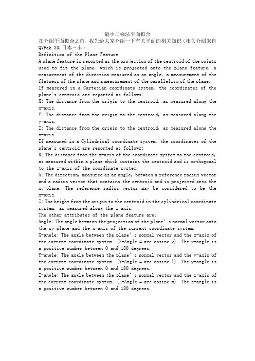
最小二乘法平面拟合在介绍平面拟合之前,我先给大家介绍一下有关平面的相关知识(相关介绍来自QVPak 3D,日本三丰)Definition of the Plane FeatureA plane feature is reported as the projection of the centroid of the points used to fit the plane, which is projected onto the plane feature, a measurement of the direction measured as an angle, a measurement of the flatness of the plane and a measurement of the parallelism of the plane.If measured in a Cartesian coordinate system, the coordinates of the plane's centroid are reported as follows:X: The distance from the origin to the centroid, as measured along the x-axis.Y: The distance from the origin to the centroid, as measured along the y-axis.Z: The distance from the origin to the centroid, as measured along the z-axis.If measured in a Cylindrical coordinate system, the coordinates of the plane's centroid are reported as follows:R: The distance from the z-axis of the coordinate system to the centroid, as measured within a plane which contains the centroid and is orthogonal to the z-axis of the coordinate system.A: The direction, measured as an angle, between a reference radius vector and a radius vector that contains the centroid and is projected onto the xy-plane. The reference radius vector may be considered to be the x-axis.Z: The height from the origin to the centroid in the cylindrical coordinate system, as measured along the z-axis.The other attributes of the plane feature are:Angle: The angle between the projection of the plane’s normal vector onto the xy-plane and the x-axis of the current coordinate system.X-angle: The angle between the plane’s normal vector and the x-axis of the current coordinate system. (X-Angle = arc cosine k). The x-angle is a positive number between 0 and 180 degrees.Y-angle: The angle between the plane’s normal vector and the y-axis of the current coordinate system. (Y-Angle = arc cosine l). The y-angle is a positive number between 0 and 180 degrees.Z-angle: The angle between the plane’s normal vector and the z-axis of the current coordinate system. (Z-Angle = arc cosine m). The z-angle is a positive number between 0 and 180 degrees.Flatness: Flatness is a condition for which an element of a surface is in a plane.Flatness is reported as the width of the zone formed by two closest parallel planes that fully contain the point set used to fit the plane feature. A value of zero indicates perfect flatness.Flatness (minimum): The distance from the fitted plane to the measured point farthest below the fitted plain in the point set. Above and below are determined by the direction of the plane vector. See Explanation of Max/Min distance in different cases.Flatness (maximum): The distance from the fitted plane to the measured point farthest above the fitted plain in the point set. Above and below are determined by the direction of the plane vector. See Explanation of Max/Min distance in different cases.Parallelism: The condition of a feature, projected to a certain plane, being equidistant at all elements from a datum (reference). Quantitatively, parallelism is defined as the absolute distant difference between the farthest and closest points from the datum.Parallelism is evaluated relative to a reference line or xy-plane. When evaluating a set of points with a reference line, parallelism uses the projections of the points and reference line onto the xy-plane in the current coordinate system, or z/ref plane feature, and is specified as a zone tolerance. The z/ref plane feature is a plane including the reference line and parallel to (or including) the z-axis. When evaluating a set of points with a xy-plane, parallelism is calculated in three-dimensional space.Parallelism (minimum): The distance from the referenced line or plane to the point in the point set with the least value (least positive value if all evaluated points are positive, or most negative value if evaluatedpoints include negative values). See Explanation of Max/Min distance in different cases.Parallelism (maximum): The distance from the reference line or plane to the point in the point set with the greatest value (most positive value if evaluated points include positive values, or least negative value if all evaluated points are negative). See Explanation of Max/Min distance in different cases.平面相关知识:算法如下:VB源代码:Option ExplicitPublic Const PI = 3.97Public Type tagPointx As Doubley As Doublez As DoubleEnd TypePublic Type tagLine2Dk As Double 'Slope ,K is the "K" of "y=kx+b"b As Double 'intercept,B is the "B" of "y=kx+b"Angle As Double 'arctg(k) '0 to 180 degStraightness As DoubleRSQ As DoubleEnd TypePublic Type tagLine3D'3D line's formula is showing as following.'1)|Ax +By +Z+D =0' |A1x+B1y+z+D1=0'2)(x-x0)/m=(y-y0)/n=(z-z0)/p----(x-x0)/m=(y-y0)/n=z/1'3)x=mt+x0,y=nt+y0,z=pt+z0'Only point's coordinate is (a+b*Z, c+d*Z,Z),so the line's vector is {b,d,1}x As Doubley As Doublez As Doublex0 As Double ' Added on Jul.1st,2009y0 As Double ' Added on Jul.1st,2009z0 As Doublem As Double '(x-x0)/m=(y-y0)/n=(z-z0)/p ,same as :z=a+bx ,z=c+dyn As Doublep As Double 'vector s={m,n,p}Angle As DoublexAn As DoubleyAn As DoublezAn As DoubleStraightness As DoubleMinSt As DoubleMaxSt As DoubleEnd TypePublic Type tagCirclex As Doubley As Doublez As Doubler As Doubled As DoubleCircular As DoubleEnd TypePublic Type tagVectora As Doubleb As Doublec As DoubleEnd TypeType tagPlanex As Double 'The distance from the origin to the centroid, as measured along the x-axis.y As Double 'The distance from the origin to the centroid, as measured along the y-axisz As Double 'The distance from the origin to the centroid, as measured along the z-axis'Z + A*x + B*y + C =0 z's coefficient is just 1ax As Double 'coefficient of Xby As Double 'coefficient of Ycz As Doubled As Double 'Constant CAngle As DoublexAn As DoubleYAn as DoublezAn As DoubleFlat As DoubleMinFlat As DoubleEnd Type'*************************************************************' 函数名:PlaneSet' 功能:求拟合平面(相关参数)' 参数: dataRaw - tagPoint型自定义点类型(x,y,z),数组' PlaneSet – tagPlane 其值返回为平面圆相关参数' 返回值:Long型,失败为0,成功为-1'*************************************************************Public Function PlaneSet(dataRaw() As tagPoint, Plane As tagPlane) As Long 'z+Ax+BY+C=0PlaneSet = 0Dim lb As Long, ub As Long, MaxF As Double, MinF As Double, tmp As Doublelb = LBound(dataRaw): ub = UBound(dataRaw)If ub - lb + 1 < 4 Then Exit FunctionDim i As Long, n As Longn = ub - lb + 1Dim x As Double, y As Double, z As DoubleDim XY As Double, XZ As Double, YZ As DoubleDim X2 As Double, Y2 As DoubleDim a As Double, b As Double, c As Double, d As DoubleDim a1 As Double, b1 As Double, z1 As DoubleDim a2 As Double, b2 As Double, z2 As DoubleDim n1 As tagVector '{.ax,by,1} s1Dim n2 As tagVector '{0,0,N} XY plane s2Dim n3 As tagVector 'line projected planeDim SLine As tagVectorDim xLine As tagVector '{1,0,0}Dim yLine As tagVector '{1,0,0}Dim zLine As tagVector '{1,0,0}Dim VectorPlane As tagVectorxLine.a = 1: xLine.b = 0: xLine.c = 0yLine.a = 0: yLine.b = 1: yLine.c = 0zLine.a = 0: zLine.b = 0: zLine.c = 1For i = lb To ubWith dataRaw(i)x = x + .xy = y + .yz = z + .zXY = XY + .x * .yXZ = XZ + .x * .zYZ = YZ + .y * .zX2 = X2 + .x ^ 2Y2 = Y2 + .y ^ 2End WithNext iz1 = n * XZ - x * z 'e=z-Ax-By-C z=Ax+By+Da1 = n * X2 - x ^ 2b1 = n * XY - x * yz2 = n * YZ - y * za2 = n * XY - x * yb2 = n * Y2 - y ^ 2a = (z1 * b2 - z2 * b1) / (a1 * b2 - a2 * b1)b = (a1 * z2 - a2 * z1) / (a1 * b2 - a2 * b1)c = 1d = (z - a * x - b * y) / nWith Plane.x = x / (ub - lb + 1).y = y / (ub - lb + 1).z = z / (ub - lb + 1)'sum(Mi *Ri)/sum(Mi) ,Mi is mass . here Mi is seted to be 1 and .z is just the average of z.Ax = -a.By = -b.Cz = 1.d = -d 'z=Ax+By+D-----Ax+By+Z+D=0VectorPlane.a = .Ax: VectorPlane.b = .By: VectorPlane.c = 1.xAn = Intersect(VectorPlane, xLine).yAn = Intersect(VectorPlane, yLine).zAn = Intersect(VectorPlane, zLine)n1.a = .Ax: n1.b = .By: n1.c = 1SLine.a = .Ax: SLine.b = .By: SLine.c = 0.Angle = Intersect(xLine, SLine) '(xLine.A * SLine.A + xLine.A * SLine.B + xLine.C * SLine.C)If SLine.b < 0 Then .Angle = 360 - .AngleFor i = lb To ubPointToPlane dataRaw(i), Plane, tmp, 0If i = lb ThenMaxF = tmp: MinF = tmpElseIf MaxF < tmp Then MaxF = tmpIf MinF > tmp Then MinF = tmpEnd IfNext i.MaxFlat = MaxF.MinFlat = MinF.Flat = MaxF - MinFEnd WithPlaneSet = -1End Function' 函数名:VectorMulti' 功能:求两向量的积,结果存放于参数rtV3中' 参数: v1 - tagVector' v2 - tagVector' rtV3 -tagVector'*************************************************************Public Function VectorMulti(v1 As tagVector, v2 As tagVector, rtv3 As tagVector) As Long'rtV3=v1*v2=|i j k |'|v1.A v1.B v1.C|'|v2.A v2.B v2.C|'rtv3.A=(v1.B*v2.c-v2.B*v1.C) 'i'rtV3.B=-(v1.A*v2.C-v2.A*v1.C) 'j'rtV3.C=(v1.A*v2.B-v2.A*V1.B) 'krtv3.a = (v1.b * v2.c - v2.b * v1.c)rtv3.b = -(v1.a * v2.c - v2.a * v1.c)rtv3.c = (v1.a * v2.b - v2.a * v1.b)End Function'************************************************************' 函数名:VectorN' 功能:求两向量的数量积,结果存放于参数rtV3中' 参数: v1 - tagVector' v2 - tagVector' rtV3 -tagVector'*************************************************************Public Function VectorN(v1 As tagVector, v2 As tagVector, rtv3 As tagVector) As Longrtv3.a = v1.a * v2.artv3.b = v1.b * v2.brtv3.c = v1.c * v2.cEnd Function'*************************************************************' 函数名:Intersect' 功能:求两向量之间的夹角' 参数: v1 - tagVector' v2 - tagVector' LinePlane -long 0:表示两直线之间的夹角,其它值:表示如线与平面之间,平面与平面之间的夹角(0~90)' 返回值:Double型,单位:度.'*************************************************************Public Function Intersect(v1 As tagVector, v2 As tagVector, Optional LinePlane As Long = 0) As Double'LinePlane 0 :line -line ,1:line --PlaneDim tmp As Double, tmpSqr1 As Double, tmpSqr2 As Doubletmp = (v1.a * v2.a + v1.b * v2.b + v1.c * v2.c)'MsgBox tmptmpSqr1 = Sqr(v1.a ^ 2 + v1.b ^ 2 + v1.c ^ 2)tmpSqr2 = Sqr(v2.a ^ 2 + v2.b ^ 2 + v2.c ^ 2)If tmpSqr1 <> 0 ThenIf tmpSqr2 <> 0 Thentmp = tmp / tmpSqr1 / tmpSqr2Elsetmp = tmp / tmpSqr1End IfElseIf tmpSqr2 <> 0 Thentmp = tmp / tmpSqr2Elsetmp = 0End IfEnd IfIf LinePlane <> 0 Thentmp = Abs(tmp)End IfIf -tmp * tmp + 1 <> 0 Thentmp = Atn(-tmp / Sqr(-tmp * tmp + 1)) + 2 * Atn(1)tmp = tmp / PI * 180Elsetmp = 90End IfIntersect = tmpEnd Function'*************************************************************' 函数名:PointToPlane' 功能:求点到平面的距离' 参数: dataRaw - tagPoint型自定义点类型(x,y,z)' Plane - tagPlane Double' RtnDistance -Double 其值为点到直线的距离. ' AbsDist -Long 0:点到平面距离(有正有负),其它值:点到平面距离(绝对值)' 返回值:Long型,失败为0,成功为-1'*************************************************************Public Function PointToPlane(dataRaw As tagPoint, Plane As tagPlane, rtnDistance As Double, Optional AbsDist As Long = 0) As Long Dim i As Long, lb As Long, ub As Long, tmp As DoubleWith Planetmp = (.ax *dataRaw.x + .by *dataRaw.y + .cz * dataRaw.z + .d)/ Sqr(.ax ^ 2 + .by ^ 2 + .cz ^ 2)If AbsDist <> 0 Thentmp = Abs(tmp)End IfEnd WithrtnDistance = tmpEnd Function'*************************************************************' 函数名:PointToLine' 功能:求点到直线的距离' 参数: dataRaw - tagPoint型自定义点类型(x,y,z)' nLine3D - tagLine3D Double' RtnDistance -Double 其值为点到直线的距离. ' 返回值:Long型,失败为0,成功为-1'*************************************************************Public Function PointToLine(dataRaw As tagPoint, nLine3D As tagLine3D, rtnDistance As Double) As LongDim tmp As Double, d As Double, t As DoubleDim Dataraw0 As tagPointWith nLine3D'直线{m,n,1}为平面:ax+by+z+d=0的法线,所以平面法线向量{a,b,1}={m,n,1}'点(dataRaw)过平面:ax+by+z+d=0, 求出dd = -.m * dataRaw.x - .n * dataRaw.y - .p * dataRaw.z '.p=1'直线与平面相交,将(x-xo)/m=(y-y0)/n=z=t ' x=m*t+x0 ; y=n*t+yo z=t 代入平面, 求得tt = -(d + .m * .x0 + .n * .y0) / (.m ^ 2 + .n ^ 2 + 1)Dataraw0.x = .m * t + .x0Dataraw0.y = .n * t + .y0Dataraw0.z = .p * t + .z0rtnDistance = Sqr((Dataraw0.x - dataRaw.x) ^ 2 + _(Dataraw0.y - dataRaw.y) ^ 2 + _(Dataraw0.z -dataRaw.z) ^ 2)End With End Function。
点云最小二乘法拟合平面公式

点云最小二乘法拟合平面公式点云最小二乘法拟合平面公式是许多计算机视觉和计算机图形学应用中的一个关键问题。
下面我们将详细介绍该公式的推导和使用方法。
一、最小二乘法最小二乘法是一种用于优化拟合曲线的方法,其主要思想是通过最小化拟合函数与实际观测值之间的误差来找到最佳拟合曲线。
在点云最小二乘法拟合平面中,我们将使用最小二乘法来找到最佳平面参数。
二、点云最小二乘法拟合平面公式假设有n个三维点,分别为(x1, y1, z1), (x2, y2, z2), ..., (xn, yn, zn),我们要使用最小二乘法拟合一个平面方程z=ax+by+c。
我们可以将该方程改写为z=ax+by-c,然后将其看作一个关于未知数a、b和c的线性方程组:⎧⎪⎨⎪⎩x1 y1 1 x2 y2 1 … xn yn 1⎫⎪⎬⎪⎭⎧⎪⎨⎪⎩a b c⎫⎪⎬⎪⎭ =⎧⎪⎨⎪⎩z1 z2 … zn⎫⎪⎬⎪⎭其中,左侧系数矩阵的第i行为(xi, yi, 1),右侧常数项向量的第i个元素为zi。
我们可以使用最小二乘法求解上述线性方程组,具体方法包括计算系数矩阵的转置A^T与系数矩阵A的乘积A^T*A,然后计算矩阵的逆(A^T*A)^(-1)和A^T与常数项向量的乘积A^T*b,最后解出未知数向量x=(a,b,-c)^T,即可得到拟合平面的方程。
三、实现方法实现点云最小二乘法拟合平面公式的方法通常包括以下步骤:1. 读取点云数据,构建系数矩阵A和常数项向量b。
2. 计算矩阵A^T*A、矩阵(A^T*A)^(-1)和向量A^T*b。
3. 计算未知数向量x=A^T*A)^(-1)*A^T*b,即可得到平面方程。
4. 可以使用拟合平面方程对点云数据进行投影、重建等操作。
四、应用领域点云最小二乘法拟合平面公式广泛应用于计算机视觉和计算机图形学领域。
例如,在三维重建、点云配准、机器人导航、三维打印等方面都需要使用该公式来寻找最佳平面参数。
总之,点云最小二乘法拟合平面公式是现代计算机科学的重要组成部分,对实现一些最前沿的技术具有重要意义。
最小二乘法拟合 最小二乘法(又称最小平方法)是一种数学优化技术它通过
---------------------------------------------------------------最新资料推荐------------------------------------------------------最小二乘法拟合最小二乘法(又称最小平方法)是一种数学优化技术它通过最小二乘法拟合最小二乘法(又称最小平方法)是一种数学优化技术。
它通过最小化误差的平方和寻找数据的最佳函数匹配。
利用最小二乘法可以简便地求得未知的数据,并使得这些求得的数据与实际数据之间误差的平方和为最小。
最小二乘法还可用于曲线拟合。
其他一些优化问题也可通过最小化能量或最大化熵用最小二乘法来表达。
对给定数据点{(Xi,Yi)}(i=0,1,,m),在取定的函数类中,求p(x),使误差的平方和 E最小,E=[p(Xi)-Yi]。
从几何意义上讲,就是寻求与给定点 {(Xi,Yi)}(i=0,1,,m)的距离平方和为最小的曲线 y=p(x)。
函数 p(x)称为拟合函数或最小二乘解,求拟合函数 p(x)的方法称为曲线拟合的最小二乘法。
Matlab 程序代码disp(‘请以向量的形式输入x,y.’) x=input(‘x=‘); y=input(‘y=‘); nx = length(x); ny = length(y); n = length(x); if nx == ny x1 = x(1); xn = x(n); % n 个数据可以拟合(n-1)阶多项式,高阶多项式多次求导,数值特性变差disp(‘通过下面的交互式图形,你可以事先估计一下你要拟合的1 / 3多项式的阶数,方便下面的计算.’) disp(‘polytool()是交互式函数,在图形上方[Degree]框中输入阶数,右击左下角的[Export]输出图形’) disp(‘回车打开polytool 交互式界面’) pause; polytool(x,y,1) % 观察多项式拟合的图形,选择置信区间最小的多项式阶数disp(‘回车继续进行拟合’) pause; % (2)-----计算多项式的各项系数和拟合值m=input(‘ 输入多项式拟合的阶数 m = ‘); [p,S]=polyfit(x,y,m); disp ‘ 输出多项式的各项系数’ fprintf (1,’ a = %3.16f \n’,p) disp ‘ 输出多项式的有关信息S’ disp (S) [yh,delta]=polyconf(p,x,S); disp ‘ 观测数据拟合数据’ disp ‘ x y yh’for i = 1 : n xy = [x(i) y(i) yh(i)]; disp (xy) end % (3)-----绘制观测数据离散点图和多项式曲线plot(x,y,’r.’) title(‘\bf 实验数据离散点图 / 多项式曲线\it y = a0+a1x+a2x +a3x +...’) grid hold on; xi=[x1:0.1:xn]; yi=polyval(p,xi); plot(xi,yi,’k-’) % (4)-----拟合效果和精度检验Q=sum((y-yh).); SGM = sqrt(Q / (n - 2)); RR = sum((yh-mean(y)).)/sum((y-mean(y)). ); fprintf (1,’ 剩余平方和 Q = %3.6f \n’,Q) fprintf (‘\n’) fprintf (1,’ 标准误差 Sigma = %3.6f \n’,SGM) fprintf (‘\n’) fprintf (1,’ 相关指数 RR = %3.6f \n’,RR) fprintf (‘\n’) disp(‘请输入你所需要拟合的数据点,若没有请按回车键结束程序.’) fprintf (‘\n’) x0=input(‘ 输入插值点x0 = ‘); y0=polyval(p,x0); fprintf (1,’ 输出插值点拟合函数值 y0 = %3.4f \n’,y0) else---------------------------------------------------------------最新资料推荐------------------------------------------------------disp(‘输入的数据有误,请重新运行程序并输入正确的数据。
最小二乘拟合平面方法

最小二乘拟合平面方法《嘿,你了解最小二乘拟合平面方法不?》嘿,大家好!今天咱们来聊聊这个听上去很专业很高大上的“最小二乘拟合平面方法”。
想象一下,要是数学也能变得像咱平时唠嗑那么轻松该多好哇!其实吧,这最小二乘拟合平面方法呢,就像是一个超级厉害的“整形大师”!只不过呢,它不是给人的脸整形,而是给一堆数据整形。
咱平时不是会遇到好多的数据嘛,乱七八糟的,但又想从里面找到点规律。
这时候最小二乘拟合平面方法就闪亮登场啦!它能把这些零散的数据点变得乖乖听话,给它们整出一个平面来。
这个平面就好像是给这些数据点找到了一个舒适的“家”,让它们不再四处乱跑。
比如,你要研究房价和地理位置、房屋面积的关系,它就能帮你弄出一个平面来,让你大致搞清楚这里面的门道。
我第一次接触这个方法的时候啊,那可真是有点懵。
看着那一堆公式和计算,我脑袋都大了一圈。
心想:哎呀妈呀,这是要闹哪样啊!不过呢,等我慢慢静下心来,一点一点去理解,发现它其实也没那么恐怖啦。
就像生活中好多看起来很难的事情,只要我们鼓起勇气去面对,静下心来研究,总能找到解决的办法。
最小二乘拟合平面方法也是这样,虽然它一开始可能会让你有点头疼,但是当你搞懂了它的原理,学会了运用它,你就会发现它的神奇之处啦!而且啊,当你用它成功解决了一个问题,那种成就感简直爆棚!就好像你是个超级英雄,一下子就把那些捣乱的数据给收服了。
所以呀,别被这个方法的名字给吓到啦。
它就像一个隐藏的宝藏,等着我们去挖掘呢!大家都勇敢地去尝试尝试,说不定你会发现一个全新的数学世界哦。
嘿嘿,就让我们和这个“最小二乘拟合平面方法”愉快地玩耍吧!怎么样,是不是感觉也没那么难了呢?加油哦!。
最小二乘拟合平面直线公式
最小二乘拟合平面直线公式最小二乘法是一种常用的数据拟合方法,可以通过最小化误差平方和来找到最佳拟合函数的参数。
在平面直线拟合问题中,最小二乘法可以帮助我们找到最佳的直线拟合模型。
平面直线拟合问题是指给定一组二维数据点,我们需要找到一条直线来拟合这些点,使得拟合直线与数据点的误差最小。
这个问题可以用最小二乘法来解决。
我们需要定义拟合直线的数学模型。
假设拟合直线的方程为y = mx + b,其中m是斜率,b是截距。
我们的目标是找到最佳的斜率和截距,使得拟合直线与数据点的误差最小。
为了使用最小二乘法,我们需要定义误差的计算方法。
在平面直线拟合问题中,常用的误差计算方法是计算每个数据点到拟合直线的垂直距离的平方和。
假设数据点的坐标为(xi, yi),拟合直线的方程为y = mx + b,则第i个数据点到拟合直线的垂直距离为:di = yi - (mx + b)我们的目标是最小化所有数据点的垂直距离的平方和,即最小化以下函数:S = Σ(di^2) = Σ(yi - mx - b)^2为了找到最佳的斜率m和截距b,我们需要对S进行求导并令导数为0。
通过求导计算,我们可以得到以下两个方程:Σ(xi * di) = Σ(xi * yi) - m * Σ(xi^2) - b * Σ(xi)Σ(di) = Σ(yi) - m * Σ(xi) - nb这是一个线性方程组,其中未知数是斜率m和截距b。
通过解这个方程组,我们可以得到最佳的斜率和截距,从而得到最佳的拟合直线。
在实际应用中,我们可以使用计算软件或编程语言来求解这个线性方程组。
通过输入数据点的坐标,我们可以得到最佳的拟合直线的斜率和截距。
最小二乘拟合平面直线公式可以帮助我们在给定一组二维数据点时,找到最佳的直线拟合模型。
通过最小化误差平方和,我们可以求解得到最佳的斜率和截距,从而得到最佳的拟合直线。
这个方法在数据分析、回归分析等领域都有广泛的应用。
最小二乘线性及平面拟合原理及C++实现

最⼩⼆乘线性及平⾯拟合原理及C++实现⼀、线性最⼩⼆乘拟合使⽤⼀个简单函数在整体上逼近已知函数,使其在整体上尽可能与原始数据曲线近似。
记为:称之为拟合曲线,若该函数为插值多项式,则所有偏差为零。
但实际情况中,我们不可能要求近似曲线y =严格通过这么多数据点。
但为了使其尽可能反映所给数据的变化趋势,我们可以要求偏差的绝对值尽可能⼩,甚⾄是所有偏差中的最⼤值尽可能⼩。
我们可以通过使选取的近似曲线在节点x i处的偏差的平⽅和达到最⼩来实现这⼀⽬标,这⼀原则就是最⼩⼆乘原则。
按最⼩原则选择的拟合曲线就称为最⼩⼆乘拟合曲线,此⽅法称为最⼩⼆乘法。
实⽤公式推导:假设我们此处有这样⼀组数据点,这些点的分布接近于在⼀条直线上,因此选⼀条直线(⼀条曲线则加⼊对应⽅程推导)来拟合这组数据,令:根据最⼩⼆乘原则,有:令a0,a1为未知数,则此处转换为求⼆元函数S(a0,a1)的极⼩点问题:由此可得:联⽴解得:即得到了待求的拟合直线段。
C++实现:bool gFittingLine(double *xArray, double *yArray, int firstIndex, int lastIndex,double &a, double &b){ int count = lastIndex-firstIndex+1;if(count < 2) return false;double s0 = (double)count, s1 = 0, s2 = 0, t0 = 0, t1 = 0;for(int i=firstIndex;i<=lastIndex;i++){s1 += xArray[i];s2 += (xArray[i]*xArray[i]);t0 += yArray[i];t1 += (xArray[i]*yArray[i]);}double d = s0*s2-s1*s1;b = (s2*t0-s1*t1)/d;a = (s0*t1-s1*t0)/d;return true;} 实现对⼆维平⾯离散点的曲线拟合⼆、最⼩⼆乘⾯拟合对空间中的⼀系列散点,寻求⼀个近似平⾯,与线性最⼩⼆乘⼀样,只是变换了拟合⽅程:使⽤平⾯的⼀般⽅程:Ax + By + CZ + D = 0可以令平⾯⽅程为:由最⼩⼆乘法知:同样分别取 a0,a1,a2的偏导数:即是:换算为矩阵形式有:可以直接通过克拉默法则求出a0,a1,a2的⾏列式表达式,有:c++实现(gDaterm3() 为⾃定义的三阶⾏列式计算函数):bool gFittingPlane(double *x, double *y, double *z, int n, double &a, double &b, double &c) {int i;double x1, x2, y1, y2, z1, xz, yz, xy, r;x1 = x2 = y1 = y2 = z1 = xz = yz = xy = 0;for(i=0; i<n; i++){x1 += x[i];x2 += x[i]*x[i];xz += x[i]*z[i];y1 += y[i];y2 += y[i]*y[i];yz += y[i]*z[i];z1 += z[i];xy += x[i]*y[i];}r = gDeterm3(x2, xy, x1, xy, y2, y1, x1, y1, n);if(IS_ZERO(r)) return false;a = gDeterm3(xz, xy, x1, yz, y2, y1, z1, y1, n) / r;b = gDeterm3(x2, xz, x1, xy, yz, y1, x1, z1, n) / r;c = gDeterm3(x2, xy, xz, xy, y2, yz, x1, y1, z1) / r;return true;}。
平面拟合最小二乘法

平面拟合的最小二乘法
说起平面拟合的最小二乘法,咱四川人也得懂点科学撒。
这个方法,说白了,就是找一个最平的平面,让它尽量多地穿过或者靠近给定的那些点。
你看哈,假如手头有一堆乱糟糟的点,就像咱们吃火锅时点的那些菜,七零八落地摆在桌子上。
现在,你想用一个平面来盖住或者尽量接近这些点,咋个办呢?这时候,最小二乘法就派上用场了。
它就像是咱们四川的厨师,手艺高超,能把那些杂七杂八的点“捋顺”了,用一个平面去拟合它们。
这个平面,不是随便找的,而是要让所有点到这个平面的距离的平方和最小。
为啥子要平方和最小呢?因为这样可以保证误差的分布最均匀,不会出现大的偏差。
具体咋个操作呢?说起来也简单,就是通过数学计算,找出一个平面的方程,这个方程能让那些点到平面的距离的平方和最小。
这个方程,就是咱们要找的那个最平的平面。
最小二乘法,听起来高大上,其实原理并不复杂。
它就像是咱们四川人打麻将,虽然牌面千变万化,但总能找到一种最优的打法,让胡牌的机会最大。
同样地,最小二乘法也是通过计算,找到一种最优的平面拟合方式,让那些点尽量多地被平面“罩住”。
所以说,别看这个方法名字怪,其实它挺实用的,在很多领域都能派上用场。
咱们四川人,也得与时俱进,学点科学知识,才能更好地应对生活中的各种挑战嘛。
多点定位算法 最小二乘
多点定位算法最小二乘
多点定位算法最小二乘是一种常用于解决多点定位问题的数学
方法。
该算法的目标是通过最小化误差的平方和来估计未知点的位置。
它在无网络信息的情况下,依靠一组测量数据来计算未知点的坐标。
在多点定位问题中,我们假设已知一组已知点的坐标,以及这些
已知点到未知点的测量距离。
我们的目标是通过这些测量数据来估计
未知点的坐标。
最小二乘算法使用的原理是通过最小化测量误差的平方和来确定
未知点的位置。
通过使用迭代算法,我们可以逐步调整估计的坐标值,直到达到最小误差。
具体操作中,最小二乘算法将测量数据转化为数学方程,其中包
括未知点的坐标和测量距离。
通过建立一个误差函数,根据未知点的
坐标和测量数据计算出误差值。
然后,算法通过迭代的方式调整未知
点的坐标值,使误差函数的值逐渐趋于最小。
最小二乘算法在实际应用中有着广泛的应用。
例如,在无线定位、导航系统和地理信息系统中,多点定位算法最小二乘被用于计算GPS
接收器的位置。
它也可以应用于其他领域,如无线传感器网络和机器
人导航。
总的来说,多点定位算法最小二乘是一种有效的数学方法,用于
解决多点定位问题。
通过最小化误差的平方和,该算法可以估计未知
点的位置,具有广泛的应用价值。
- 1、下载文档前请自行甄别文档内容的完整性,平台不提供额外的编辑、内容补充、找答案等附加服务。
- 2、"仅部分预览"的文档,不可在线预览部分如存在完整性等问题,可反馈申请退款(可完整预览的文档不适用该条件!)。
- 3、如文档侵犯您的权益,请联系客服反馈,我们会尽快为您处理(人工客服工作时间:9:00-18:30)。
平面方程拟合计算
平面方程的一般表达式为:
0=+++D Cz By Ax , (0≠C )
C
D y C B x C A z ---
= 记:C D a C B a C A a -=-=-=210,, 则:210a y a x a z ++=
平面方程拟合:
对于一系列的n 个点)3(≥n :
1,,1,0),,,(-=n i z y x i i i
要用点1,,1,0),,,(-=n i z y x i i i 拟合计算上述平面方程,则使:
()∑-=-++=1
02
210n i z a y a x a S 最小。
要使得S 最小,应满足: 2,1,0,0==∂∂k a S k
即:⎪⎩⎪⎨⎧=-++=-++=-++∑
∑∑0)(20)(20)(2210210210i i i i i i i i i i i z a y a x a y z a y a x a x z a y a x a
有,⎪⎩⎪⎨⎧=++=++=++∑∑∑∑∑∑∑∑∑∑∑i
i i i i i i i i i i i i i i z n a y a x a z y y a y a y x a z x x a y x a x a 21022102120 或,⎪⎪⎪⎭⎫ ⎝
⎛=⎪⎪⎪⎭⎫ ⎝⎛∑∑∑∑∑∑∑∑∑∑∑i i i i i i i i i
i
i i i i i
z z y z x a a a n y x y y y x x y x x 21022 解上述线形方程组,得:210,,a a a
即:210a y a x a z ++=
其程序代码如下:
#include ""
#include <>
#include <>
#include <>
#define MAX 10
void Inverse(double *matrix1[],double *matrix2[],int n,double d); double Determinant(double* matrix[],int n);
double AlCo(double* matrix[],int jie,int row,int column); double Cofactor(double* matrix[],int jie,int row,int column);
int _tmain(int argc, _TCHAR* argv[])
{
double array[12][3],Y[3];
double A,B,C;
A =
B =
C = ;
ZeroMemory(array,sizeof(array));
ZeroMemory(Y,sizeof(Y));
for (int i = 0;i < 12;i++)
{
for (int j = 0;j < 3;j++)
{
array[i][j] = (double)rand();
}
}
for (int i = 0; i < 12;i++)
{
array[i][0] = ;
}//设计了12个最简单的数据点,x = 1平面上的点,
double *Matrix[3],*IMatrix[3];
for (int i = 0;i < 3;i++)
{
Matrix[i] = new double[3];
IMatrix[i] = new double[3];
}
for (int i = 0;i < 3;i++)
{
for (int j = 0;j < 3;j++)
{
*(Matrix[i] + j) = ;
}
}
for (int j = 0;j < 3;j++)
{
for (int i = 0;i < 12;i++)
{
*(Matrix[0] + j) += array[i][0]*array[i][j];
*(Matrix[1] + j) += array[i][1]*array[i][j];
*(Matrix[2] + j) += array[i][2]*array[i][j];
Y[j] -= array[i][j];
}
}
double d = Determinant(Matrix,3);
if (abs(d) <
{
printf("\n矩阵奇异");
getchar();
return -1;
}
Inverse(Matrix,IMatrix,3,d);
for (int i = 0;i < 3;i++)
{
A += *(IMatrix[0] + i)*Y[i];
B += *(IMatrix[1] + i)*Y[i];
C += *(IMatrix[2] + i)*Y[i];
}
printf("\n A = %,B = %,C= %",A,B,C);
for (int i = 0;i < 3;i++)
{
delete[] Matrix[i];
delete[] IMatrix[i];
}
getchar();
return 0;
}
void Inverse(double *matrix1[],double *matrix2[],int n,double d) {
int i,j;
for(i=0;i<n;i++)
matrix2[i]=(double *)malloc(n*sizeof(double));
for(i=0;i<n;i++)
for(j=0;j<n;j++)
*(matrix2[j]+i)=(AlCo(matrix1,n,i,j)/d);
}
double Determinant(double* matrix[],int n)
{
double result=0,temp;
int i;
if(n==1)
result=(*matrix[0]);
else
{
for(i=0;i<n;i++)
{
temp=AlCo(matrix,n,n-1,i);
result+=(*(matrix[n-1]+i))*temp;
}
}
return result;
}
double AlCo(double* matrix[],int jie,int row,int column) {
double result;
if((row+column)%2 == 0)
result = Cofactor(matrix,jie,row,column);
else result=(-1)*Cofactor(matrix,jie,row,column);
return result;
}
double Cofactor(double* matrix[],int jie,int row,int column) {
double result;
int i,j;
double* smallmatr[MAX-1];
for(i=0;i<jie-1;i++)
smallmatr[i]= new double[jie - 1];
for(i=0;i<row;i++)
for(j=0;j<column;j++)
*(smallmatr[i]+j)=*(matrix[i]+j);
for(i=row;i<jie-1;i++)
for(j=0;j<column;j++)
*(smallmatr[i]+j)=*(matrix[i+1]+j);
for(i=0;i<row;i++)
for(j=column;j<jie-1;j++)
*(smallmatr[i]+j)=*(matrix[i]+j+1);
for(i=row;i<jie-1;i++)
for(j=column;j<jie-1;j++)
*(smallmatr[i]+j)=*(matrix[i+1]+j+1);
result = Determinant(smallmatr,jie-1);
for(i=0;i<jie-1;i++)
delete[] smallmatr[i];
return result;
}。