2014年数学建模美赛题目
美国大学生数学建模比赛2014年B题

Team # 26254
Page 2 oon ............................................................................................................................................................. 3 2. The AHP .................................................................................................................................................................. 3 2.1 The hierarchical structure establishment ....................................................................................................... 4 2.2 Constructing the AHP pair-wise comparison matrix...................................................................................... 4 2.3 Calculate the eigenvalues and eigenvectors and check consistency .............................................................. 5 2.4 Calculate the combination weights vector ..................................................................................................... 6 3. Choosing Best All Time Baseball College Coach via AHP and Fuzzy Comprehensive Evaluation ....................... 6 3.1 Factor analysis and hierarchy relation construction....................................................................................... 7 3.2 Fuzzy comprehensive evaluation ................................................................................................................... 8 3.3 calculating the eigenvectors and eigenvalues ................................................................................................ 9 3.3.1 Construct the pair-wise comparison matrix ........................................................................................ 9 3.3.2 Construct the comparison matrix of the alternatives to the criteria hierarchy .................................. 10 3.4 Ranking the coaches .....................................................................................................................................11 4. Evaluate the performance of other two sports coaches, basketball and football.................................................... 13 5. Discuss the generality of the proposed method for Choosing Best All Time College Coach ................................ 14 6. The strengths and weaknesses of the proposed method to solve the problem ....................................................... 14 7. Conclusions ........................................................................................................................................................... 15
2014年AMC_12真题 (B)
(C)
75 2
(D) 40
(E)
300 7
4. Susie pays for 4 muffins and 3 bananas. Calvin spends twice as much paying for 2 muffins and 16 bananas. A muffin is how many times as expensive as a banana?
15. When p 6 , the number e p is an integer. What is the largest power of 2 that is k 1k ln k a factor of e p ? (A) 212 (B) 214 (C) 216 (D) 218 (E) 220
r and s such that the line through Q with slope m does not intersect P if and only if r < m < s. What is r + s? (A)1 (B)26 (C)40 (D)52 (E)80
18. The numbers 1, 2, 3, 4, 5 are to be arranged in a circle. An arrangement is bad if it is not true that for every n from 1 to 15 one can find a subset of the numbers that appear consecutively on the circle that sum to n. Arrangements that differ only by a rotation or a reflection are considered the same. How many different bad arrangements are there? (A) 1 (B) 2 (C) 3 (D) 4 (E) 5
2014年美国大学生数学建模竞赛MCM A题二等奖
For office use only F1 ________________ F2 ________________ F3 ________________ F4 ________________
A
Simulations of a Multi-Lane Traffic Model Using Cellular Automata Concerning the Overtaking Effect
Summary
The prosperity of modern industrialized world is largely depend on today’s sophisticated road networks. The rapid growth of vehicle number often exceeds the capacity of existing road [1,2]. Thus the effective utilization of road capacity is indispensable in traffic flow control. Cellular automaton model (CA model) is an very practical model in stimulating traffic flow behavior. This paper aims at building a CA model for multi-lane traffic using right-most overtaking law. The first CA model is the well-known NaSch model[9] Knospe studied a two-lane model focus on the density dependence of lane changes[10,11]. A numerical approach is performed by Daoudia and Moussa to stimulate the 3-lane traffic flow[12]. Basing upon the previous done by [1,9,10,12], we put forward an extended CA model using right-most overtaking rule. By a detailed investigation on overtaking process, we obtain the least safe distance under different speed limits and traffic flow densities, due to the limitation of least safe distance, we put forward incentive and safety criteria of overtaking behavior for particles on different lanes in our CA model. Simulation of our model is performed for three-lane case, and the result shows that our right-most overtaking rule behaves asymmetrically such that the right-most lane firstly reach at the “critical density” where the traffic flow reaches its peak point. And despite the special behavior of our own model, our results indicate a robust behavior of traffic flow such that when traffic density is roughly 0.1, the traffic flow arrives at its peak value, and with an increase of particle density, the phase transition occurs such that the traffic jams and “stop-and-go” phenomena happens. This result is of significance in conducting the daily traffic flow in our real world. Keywords: traffic flow, cellular automaton, right-most overtaking, simulation
2014数模美赛A
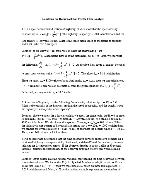
Solutions for Homework for Traffic Flow Analysis1. On a specific westbound section of highway, studies show that the speed-density relationship is: ])(1[5.3jf k k u u -=. The highway’s capacity is 3800 vehicles/hour and the jam density is 140 vehicles/km. What is the space mean speed of the traffic at capacity and what is the free flow speed.Solution: as we know q = ku, thus, we can write the following: q = ku = k*])(1[5.3jf k k u -. When traffic flow is at the maximum, dq/dk = 0. Thus, we can write the following: 0]15.41[5.35.3=⨯-=k k u dk dq jf . As the free-flow speed u f can not be equal to zero, thus, we can write: 0]15.41[5.35.3=⨯-k k j . Therefore, k m = 91.1 vehicles/km.Since we know q m = 3800 vehicles/hour. And again, q m = k m u m , then we can calculate u m= 41.7 km/hour. Then, we can calculate u f from the given equation: ])(1[5.3jf k k u u -=. In the end, we may obtain: u f = 53.5 km/hr.2. A section of highway has the following flow-density relationship: q = 80k – 0.4k 2. What is the capacity of the highway section, the speed at capacity, and the density when the highway is one-quarter of its capacity?Solution: since we know the q-k relationship, we apply the same logic: dq/dk = 0 in order to obtain k m . (dq/dk) = 80-0.8k = 0, thus, k m = 100 vehicles/km. We can also obtain q m = 4000 vehicles/hour. We also know that q = km. Then, u m = q m /k m = 40 km/hour. When the highway is one quarter of its capacity, it means that q = 0.25q m = 1000 vehicles/hour, we can use the given equation: q = 80k – 0.4k 2, to calculate the density when q = (1/4)q m . Thus, k = 186 km/hour or 13.8 km/hour.3. An observer has determined that the time headways between successive vehicles on a section of highway are exponentially distributed, and that 60% of the headways between vehicles are 13 seconds or greater. If the observer decides to count traffic in 30 second intervals, estimate the probability of the observer counting exactly four vehicles in an interval.Solution: let us denote h as the random variable, representing the time headways between successive vehicles. We know that Pr(h ≥ 13) = 0.6. In other words, if we set t = 13, we know that Pr(h ≥ 13) = e -λ*13, then we can calculate λ based on these two equations. λ = 0.039 vehicles/second. Now, let X be the random variable representing the number ofvehicle arrivals during time t, then X is poisson distributed. Pr(X=4) ==⨯=⨯--!4)30039.0(!)(30039.4e x e t t x λλ0.024.4. A vehicle pulls out onto a single-lane highway that has a flow rate of 280 vehicles/hour (poisson distributed). The driver of the vehicle does not look for oncoming traffic. Road conditions and vehicle speeds on the highway are such that it takes 1.5 seconds for an oncoming vehicle to stop once the brakes are applied. Assuming that a standard driver reaction time is 2.5 seconds, what is the probability that the vehicle pulling out will be in an accident with oncoming traffic?Solution: in this case, if the vehicle headways between successive vehicles are greater than 4 seconds, then the driver pulling out will not be in an accident. Or say, if the headways are less than 4 seconds, the driver pulling out will be in an accident.Since q = 280 vehicles/hour, then λ = 0.078 vehicles/second.Pr(h < 4) = 1-e -λt = 1-e -0.078*4 = 0.268.5. Reconsider the problem 4 above, how quick would the driver reaction times of oncoming vehicles have to be to have the probability of an accident equal to 0.15?Solution: let t denote the new driver reaction time. So,Pr[h < (1.5+t)] = 1 – e -0.078*(1.5+t) = 0.15, then, we can obtain t = 0.58.In other words, to reduce the probability of an accident to 0.15, the driver reaction must be less than 0.58 seconds.6. A toll booth on a turnpike is open from 8:00 am to 12 midnight. Vehicles start arriving at 7:45 am at a uniform deterministic rate of 6 per minute until 8:15 am and from then on at 2 per minute. If vehicles are processed at a uniform deterministic rate of 6 per minute, determine when the queue will dissipate, total delay, longest queue length (in vehicles), longest vehicle delay under first-in and first-out rule.Solutions: arrival rate λ1 = 6 vehicles/minute from 7:45 am to 8:15 am. λ2 = 2vehicles/minute from 8:15 am to the rest of the day. Departure rate μ = 2 vehicles/minute.Solution: the time when the queue will dissipate is then the arrival curve intersects with the departure curve. Q1 = 6t; Q2 = 120+2t; Q3 = -90 + 6t, where Q1 is the arrival curve between 7:45 am to 8 am and Q2 is the arrival curve starting from 8:15 am to the rest of the day and Q3 is the departure curve. By setting Q2 = Q3, we can obtain the value for t, the time when the queue dissipates, we obtain that t = 52.5 minutes. In other words, at 8:375 am, the queue completely dissipates.Because Q2 and Q3 are parallel to each other, the long delay happens anywhere on the Q1 curve and it is equal to 15 minutes. This means that every car arriving between 7:45 am to 8:15 am has to wait for 15 minutes in the queue. Also because Q2 and Q3 areparallel, the queue length is uniform between 7:45 am to 8:15 am too. The queue length is equal to 90 vehicles (Q1=6t = 6*15 = 90 vehicles).To calculate the total delay, we simply do the following:8 am 7:45 am 8:15 amTotal delay = ⎰+--⎰++⎰5.52155.5230300)690()2120(6dt t dt t tdt= 5.521525.523023002|)390(|)120(|3t t t t t +--++ = )155.52(*3)155.52(*90)305.52()305.52(*120)030(322222---+-+-+-= 2700 + 2700 + 1856.25 + 3375 – 7953.5 = 3037.5 vehicle-minutes.7. Vehicles begin to arrive at a toll booth at 8:50 am, with an arrival rate of λ(t) = 4.1 + 0.01t (with t in minutes and λ(t) in vehicles per minute). The toll booth opens at 9:00 am and process vehicles at a rate of 12 per minute throughout the day. Assume D/D/1 queuing, when will the queue dissipate and what will be the total vehicle delay? Solution: we follow the same procedure as applied in problem number 6. The arrival curve is equal to λt = 4.1t + 0.01t2 and departure curve is equal to –120 + 12t. Setting the departure curve to be equal to the arrival curve, we obtain that t = 15 minutes or 774 minutes. We take the first value, which is equal to 15 minutes.About the total delay, we integrate the arrival curve and the departure curve and substract the latter from the former, and we obtain:Total delay = 2.05t2|(0,15) + (1/300)t3 (0,15) + 120t|(10,15) – 6t2|(10,15)= 322.5 vehicle-m.。
HIMCM 2014美国中学生数学建模竞赛试题

HIMCM 2014美国中学生数学建模竞赛试题Problem A: Unloading Commuter TrainsTrains arrive often at a central Station, the nexus for many commuter trains from suburbs of larger cities on a “commuter” line. Most trains are long (perhaps 10 or more cars long). The distance a passenger has to walk to exit the train area is quite long. Each train car has only two exits, one near each end so that the cars can carry as many people as possible. Each train car has a center aisle and there are two seats on one side and three seats on the other for each row of seats.To exit a typical station of interest, passengers must exit the car, and then make their way to a stairway to get to the next level to exit the station. Usually these trains are crowded so there is a “fan” of passengers from the train trying to get up the stairway. The stairway could accommodate two columns of people exiting to the top of the stairs.Most commuter train platforms have two tracks adjacent to the platform. In the worst case, if two fully occupied trains arrived at the same time, it might take a long time for all the passengers to get up to the main level of the station.Build a mathematical model to estimate the amount of time for a passenger to reach the street level of the station to exit the complex. Assume there are n cars to a train, each car has length d. The length of the platform is p, and the number of stairs in each staircase is q. Use your model to specifically optimize (minimize) the time traveled to reach street level to exit a station for the following:问题一:通勤列车的负载问题在中央车站,经常有许多的联系从大城市到郊区的通勤列车“通勤”线到达。
2014美国数学建模竞赛赛题翻译
问题A:右行左超规则在美国、中国和大多数除了英国、澳大利亚和一些前英国殖民地的国家,多车道高速公路常常有这样一种规则。
司机必须尽量在最右的车道行使,只有超车时,司机才可以向左移动一个车道来达成目的。
当司机超车完毕后必须回到原车道继续行使。
建立并分析一个数学模型,使得这个模型能够分析这个规则在交通高负荷和低负荷情况下的表现。
你可以从许多角度来思考这个问题,比如车流量和车辆安全之间的权衡,或者一个过快或过慢的车辆限速带来的影响等等。
这个规则可以使我们获得更好的交通流?如果不可以,请提出并分析一个替代方案使得交通流得到优化、安全得到保障、或者其他你认为重要的因素得到实现。
在靠左行使才是规则的国家,论证你的解决方案是否可以通过简单的变换或者通过增加一些新的要求来解决相同的问题。
最后,以上的规则的实行是建立在人们遵守它的基础上的,然而不是所有人都愿意去遵守。
那么现在我们使同一条道(可以只是一段,也可以是全段公路)上的交通车辆都在一个智能系统的严格控制下,这个变化对你之前的分析结果有多大的影响?问题B:体育画刊是一个为体育爱好者们设计的杂志。
这个杂志正在寻找上世纪女性或者男性的“历来最优秀的大学教练”。
建立一个数学模型,从男性或者女性体育教练中选择最好的大学教练(退役或者在役的都可以)。
这些体育教练可以是大学曲棍球、陆上曲棍球、足球、橄榄球、棒球、排球、篮球的教练。
你选择划分的时间会对你的分析有影响吗?也就是说,1913年的教练方式和2013年的会有什么不同吗?清楚的阐述你的评估方式。
讨论你的模型如何通用于两性教练和所有可能的运动项目上。
用你的模型为三项体育项目分别找到五个最佳教练。
再为体育画刊提供一篇1-2页的不涉及技术性问题解释的通俗易懂的文章来解释你们的结果,你们必须保证体育爱好者们能够理解。
2014建模美赛B题
For office use onlyT1________________ T2________________ T3________________ T4________________ Team Control Number27820Problem ChosenBFor office use onlyF1________________F2________________F3________________F4________________ 2014Mathematical Contest in Modeling (MCM/ICM) Summary Sheet(Attach a copy of this page to your solution paper.)Research on Choosing the Best College Coaches Based on Data Envelopment AnalysisSummaryIn order to get the rank of coaches in differ ent sports and look for the ―best all time college coach‖ male or female for the previous century, in this paper, we build a comprehensive evaluation model for choosing the best college coaches based on data envelopment analysis. In the established model, we choose the length of coaching career, the number of participation in the NCAA Games, and the number of coaching session as the input indexes, and choose the victory ratio of games, the number of victory session and the number of equivalent champion as the output indexes. In addition, each coach is regarded as a decision making unit (DMU).First of all, with the example of basketball coaches, the relatively excellent basketball coaches are evaluated by the established model. By using LINGO software, the top 5 coaches are obtained as follows: Joe B. Hall, John Wooden, John Calipari, Adolph Rupp and Hank Iba.Secondly, the year 1938 is chosen as a time set apart to divide the time line into two parts. And then, basketball coaches are still taken as an example to evaluate the top 5 coaches used the constructed model in those two parts, respectively. The evaluated results are shown as: Doc Meanwell, Francis Schmidt, Ralph Jones, E.J. Mather, Harry Fisher before 1938, and Joe B. Hall, John Wooden, John Calipari, Adolph Rupp and Hank Iba after 1938. These results are accordant with those best coaches that were universally acknowledged by public. It suggests that the model is valid and effective. As a consequence, it can be applied in general across both genders and all possible sports.Thirdly, just the same as basketball coaches, football and field hockey coaches are also studied by using the model. After the calculation, the top 5 co aches of football’s results are as follows: Phillip Fulmer, Tom Osborne, Dan Devine, Bobby Bowden and Pat Dye, and field hockey’s are Fred Shero, Mike Babcock, Claude Julien, Joel Quenneville and Ken Hitchcock.Finally, although the top 5 coaches in each of 3 different sports have been chosen, the above-mentioned model failed to sort these coaches. Therefore, the super- efficiency DEA model is introduced to solve the problem. This model not only can evaluate the better coaches but also can rank them. As a result, we can choose the ―best all time college coach‖ from all the coaches easily.Type a summary of your results on this page. Do not includethe name of your school, advisor, or team members on this page.Research on Choosing the Best College Coaches Based on DataEnvelopment AnalysisSummaryI n order to get the rank of coaches in different sports and look for the ―best all time college coach‖ male or female for the previous century, in this paper, we build a comprehensive evaluation model for choosing the best college coaches based on data envelopment analysis. In the established model, we choose the length of coaching career, the number of participation in the NCAA Games, and the number of coaching session as the input indexes, and choose the victory ratio of games, the number of victory session and the number of equivalent champion as the output indexes. In addition, each coach is regarded as a decision making unit (DMU).First of all, with the example of basketball coaches, the relatively excellent basketball coaches are evaluated by the established model. By using LINGO software, the top 5 coaches are obtained as follows: Joe B. Hall, John Wooden, John Calipari, Adolph Rupp and Hank Iba.Secondly, the year 1938 is chosen as a time set apart to divide the time line into two parts. And then, basketball coaches are still taken as an example to evaluate the top 5 coaches used the constructed model in those two parts, respectively. The evaluated results are shown as: Doc Meanwell, Francis Schmidt, Ralph Jones, E.J. Mather, Harry Fisher before 1938, and Joe B. Hall, John Wooden, John Calipari, Adolph Rupp and Hank Iba after 1938. These results are accordant with those best coaches that were universally acknowledged by public. It suggests that the model is valid and effective. As a consequence, it can be applied in general across both genders and all possible sports.Thirdly, just the same as basketball coaches, football and field hockey coaches are also studied by using the model. After the calculation, the top 5 coaches of football’s results are as follows: Phillip Fulmer, Tom Osborne, Dan Devine, Bobby Bowden and Pat Dye, and field hockey’s are Fred Shero, Mike Babcock, Claude Julien, Joel Quenneville and Ken Hitchcock.Finally, although the top 5 coaches in each of 3 different sports have been chosen, the above-mentioned model failed to sort these coaches. Therefore, the super- efficiency DEA model is introduced to solve the problem. This model not only can evaluate the better coaches but also can rank them. As a result, we can choose the ―best all time college coach‖ from all the coaches easily.Key words: college coach;data envelopment analysis; decision making unit; comprehensive evaluationContents1. Introduction (4)2. The Description of Problem (4)3. Models (5)3.1Symbols and Definitions (5)3.2 GeneralAssumptions (6)3.3 Analysis of the Problem (6)3.4 The Foundation of Model (6)3.5 Solution and Result (8)3.6 sensitivity analysis (17)3.7 Analysis of the Result (19)3.8 Strength and Weakness (19)4.Improved Model............................................................................................................................ .. (20)4.1super- efficiency DEA model (20)4.2 Solution and Result (21)4.3Strength and Weakness (25)5. Conclusions (25)5.1 Conclusions of the problem...............................................................................,.25 5.2 Methods used in our models (26)5.3 Applications of our models (26)6.The article for Sports Illustrated (26)7.References (28)I. IntroductionAt present, the scientific evaluation index systems related to college coach abilities are limited, and the evaluation of coach abilities are mostly determined by the sports teams’game results, and it lacks of systematic, scientific and accurate evaluation with large subjectivity and one-sidedness, thus it can not objectively reflect the actual training level of coaches. In recent years, there appear many new performance evaluation methods, which mostly consider the integrity of the evaluation system. Thus they overcome a lot of weaknesses that purely based on the evaluation of game results. However, it is followed by the complexity of evaluation process and index system, as well as the great increase of the implementation cost. Data envelopment analysis is a non-parametric technique for evaluating the relative efficiency of a set of homogeneous decision-making units (DMUs) with multiple inputs and multiple outputs by using a ratio of the weighted sum of outputs to the weighted sum of inputs. Therefore, it not only simplifies the number of indexes, but also avoids the interference of subjective consciousness, thus makes the evaluation system more just and scientific.Based on the investigation and research of the US college basketball coach for the previous century, this paper aims at establishing a scientific and objective evaluation index system to assess their coaching abilities comprehensively. It provides reference for the relating sports management department to evaluate coaches and continuously optimize their coaching abilities. For this purpose, the DEA is successfully introduced into this article to establish a comprehensive evaluation model for choosing the best college coaches. It makes the assessment of the coaches in different time line horizon, different gender and different sports to testify the validity and the effectiveness of this approach.II. The Description of the Problem In order to find out the ―best all time college coach‖ for the previous century, a comprehensive evaluation model is needed to set up. Therefore, a set of scientific and objective evaluation index system should be established, which should meet the following principles or requirements:The principle of sufficiency and comprehensivenessThe index system should be sufficiently representative and comprehensivelycover the main contents of the coaches’ coaching abilities.The principle of independenceEach of the index should be clear and comparatively independent.The principle of operabilityThe data of index system comes from the existing statistics data, thus copying the unrealistic index system is not allowed.The principle of comparabilityThe comparative index should be used as far as possible to be convenientlycompared for each coach.After the establishment of evaluation index system, it requires the detailed model to make assessment and analysis for each coach. Currently, the comprehensive assessment is mostly widely used, but most of them need to be gave a weight. It is more subjective and not very scientific and objective. To avoid fixing the weight, the DEA method is adopted, which can figure out coaches’ rank eventually from the coach’s actual data.For the different time line horizon, the coaches’ rank is inevitably influenced by the team’s l evel and the sports, thus it requires discussion in different time line horizon to get the further results.Finally, the DEA model is applied to all coaches (either male or female) and all possible sports to get the rank, and then the model’s whole assessm ent basis and process should be explained to the readers in understandable words.III. Models3.1 Terms Definitions and Symbols Symbol ExplanationDMU k the k th DMU0DMU the target DMU, which is one of the nevaluated DMUs;ik x the i th input variable consumed0i x the i th input variable consumedjk y the j th output variable produced0j y the j th output variable produced1I The length of coaching career2I The number of taking part in NCAAtournament3I coaching session1Ovictory ratio of game3.2 General AssumptionsThe same level game difficulty in different regions and cities is equal for all teams.The value of the champion in different regions and cities is equal (without regard to team’s number in the region, the power and strength of the teams and other factors).The same game’s value is equal in different years (without regard to the team number in the year and other factors).The college’s level has no influence to the coach’s coaching performance.3.3 Analysis of the ProblemFor the current problem, first of all, a comprehensive evaluation model is needed to set up. Therefore, a set of scientific and objective evaluation index system should be established. The evaluation system of the coaches is comparatively mature, but it mainly based on the people’s subjective consciousness, thus the evaluation system we build requires more data to explain the problem, and it tries to assess each coach in a objective and just way without the interference of subjective factors.Secondly, the evaluation system we used is different due to the different games in different time periods. So the influence of different time periods to the evaluation results should be taken into account when we deal with the problem. Furthermore, it should be discussed in different cases.3.4 The Foundation of ModelData Envelopment Analysis (DEA), initially proposed by Charnes, Cooper and Rhodes [3], is a non-parametric technique for evaluating the relative efficiency of a set of homogeneous decision-making units (DMUs) with multiple inputs and multiple outputs by using a ratio of the weighted sum of outputs to the weighted sum of inputs. 2O the number of victory session3O The number of equivalent champion1Q the number of regular games champion2Q the number of league games champion3Qthe number of NCAA league gameschampionOne of the basic DEA models used to evaluate DMUs efficiency is the input-oriented CCR model, which was introduced by Charnes, Cooper and Rhodes [1]. Suppose that there are n comparatively homogenous DMUs (Here, we look upon each coach as a DMU), each of which consumes the same type of m inputs and produces the same type of s outputs. All inputs and outputs are assumed to be nonnegative, but at least one input and one output are positive.DMU k : the k th DMU, 1,2,,=k n ;0DMU : the target DMU, which is one of the n evaluated DMUs;ik x : the i th input variable consumed by DMU k , 1,2,,=i m ; 0i x : the i th input variable consumed by 0DMU , 1,2,,=i m ;jk y : the j th output variable produced by DMU k , 1,2,,=j s ;0j y : the j th output variable produced by 0DMU , 1,2,,=j s ; i u : the i th input weight, 1,2,,=i m ;In DEA model, the efficiency of 0DMU , which is one of the n DMUs, isobtained by using a ratio of the weighted sum of outputs to the weighted sum of inputs under the condition that the ratio of every entity is not larger than 1. The DEA model is formulated by using fractional programming as follows:()()000111112121,1,2,...,..,,,0,,,0max sr rj r m j i ij i sr rj r m i ij i T m T s j n s t v v v v u u u u y u hv x y u v x =====⎧⎪⎪≤=⎪⎪⎨⎪=≥⎪⎪=≥⎪⎩∑∑∑∑ (2)The above model is a fractional programming model, which is equivalent to the following linear programming model:00111010,1,2,...,..1,0,1,2,..;1,2,...,max s j r rj r sm i ij r rj r i m i ij i ir j n s t i m r sy h y w x w x w μμμ=====⎧-≤=⎪⎪⎪=⎨⎪⎪≥==⎪⎩∑∑∑∑ (3) Turned to another form is:101min ..0,1,2,,nj j j n j j j j x x s t j ny y θλθθλλ==⎧≤⎪⎪⎪⎪≥⎨⎪⎪≥=⎪⎪⎩∑∑无约束 3.5 Solution and Result3.5.1 Establishing the input and output index systemIn the DEA model, it requires defining a set of input index and a set of output index, and all the indexes should be the common data for each coach. Regarding the team as an unit, then the contribution that the coach made to the team can be regarded as input, while the achievement that the team made can be regarded as reward. In the following, we take the basketball coaches of NACC as an example to establish the input and output index system. These input indexes could be chosen as follows:1I :The length of coaching careerThe more game seasons a coach takes part in, the more abundant experience he has. This ki nd of coach’s achievement is easily affirmed by others. As the Figure 1 shows, the famous coach mostly experienced the long-time coaching career.Furthermore, the time the coach has contributed to the team is fundamental if they want to have a good result in the game. Thus the length of coaching career can be regarded as an index to evaluate the coach’s contribution to the team.Figure 1 The relationship between the length of coaching career and the number ofchampionsI: The number of taking part in NCAA tournament2Whether the coach takes the team to a higher level game has a direct influence on the team’s performance, and also it can reflect the coach’s coaching abilities, level and other factors.I: coaching session3For the reason of layers of elimination, the coaching session is not necessarily determined by the length of coaching career. It can be shown in the comparison between Figure 2 and Figure 3. Thus the number of coaching session can also be regarded as an index.Figure 2These output indexes could be chosen as follows:O: victory ratio of game1The index reflects the coach’s ability of command and control, and it a ttaches great importance to the evaluation of coach’s coaching abilities.O: the number of victory session2The case that the number of victory session reflected is different from that of victory ratio, only if get the enough number of victory session in a large number of coaching session, the acquired high victory ratio can reflect the coach’s high coaching level. If the victory occurs in a limited games, this kind of high victory ratio can not reflect the rules. It can be shown in the comparison between Figure 3 and Figure 4.Figure 3Figure 43O :The number of equivalent championThe honor that US college basketball teams acquired can be divided into three types: 1Q : the number of regular games champion; 2Q : the number of league games champion; 3Q : the number of NCAA league games champion. The threechampionship honor has different levels, and their importance is increasing in turn according to the reference. The weight 0.2、0.3、0.5 can be given respectively, and the number of equivalent champion can be figured out and used as an output index, as it shown in Table 1.5.0Q 3.0Q 2.0Q O 3213⨯+⨯+⨯=Table 1 Coach names Number of regular games champion (weight 0.2) Number of league games champion (weight 0.3) Number of NCAA league games championNumber of equivalent championAccording to Internet, the data of input and output are given by Table 2.Table 2(weight 0.5)Phog Allen 24 0 1 5.3 Fred Taylor 7 0 1 1.9 Hank Iba 15 0 2 4 Joe B. Hall 8 1 1 2.4 Billy Donovan 7 3 2 3.3 Steve Fisher 3 4 1 2.6 John Calipari 14 11 1 6.6 Tom Izzo 7 3 1 2.8 Nolan Richardso 9 6 1 3.9 John Wooden 16 0 10 8.2 Rick Pitino 9 11 2 6.1 Jerry Tarkanian 18 8 1 6.5 Adolph Rupp 28 13 4 11.5 John Thompson 7 6 1 3.7 Jim Calhoun 16 12 3 8.3 Denny Crum 15 11 2 7.3 Roy Williams 15 6 2 5.8 Dean Smith 17 13 2 8.3 Bob Knight 11 0 3 3.7 Lute Olson 13 4 1 4.3 Mike Krzyzewski 12 13 4 8.3 Jim Boeheim 11 5 1 4.2 Doc Meanwell 10 0 0 2 Ralph Jones 4 0 0 0.8 Francis Schmidt61.2Coach namesInput indexOutput index1I2I3I1O 2O3ONCAA tourament Thelength of coaching careerCoaching session Win-Lose %WinsNumber of equivalent championPhog Allen 4489780.735 719 5.3 Fred Taylor 5 18 455 0.653 297 1.9 Hank Iba84010850.6937524Since the opening of NACC tournament in 1938, thus the year 1938 is chosen as a time set apart. The finishing time point of coaching before 1938 is a period of time, while after 1938 is another period of time.For the time period before 1938, take the length of coaching career 1I , coaching session 3I as input indexes, and then take W-L %1O , victory session 2O , the number of regular games champion 1Q as output indexes. The results is shown in Table 3 after the data statistics of each index.For the time period after 1938, because they all take part in NACC, the input index and output index are just the same as that of all time period. The data statistics is just as shown in Table 3.Table 3Coach namesInput indexOutput index1I3I1O2O1QThe lengthof coachingcareerCoachingsessionW-L % WinsNumber of regular games championJoe B. Hall 10 16 463 0.721 334 2.4 Billy Donovan 13 20 658 0.714 470 3.3 Steve Fisher 13 24 739 0.658 486 2.6 John Calipari 14 22 756 0.774 585 6.6 Tom Izzo 16 19 639 0.717 458 2.8 Nolan Richardson 16 22 716 0.711 509 3.9 John Wooden 16 29 826 0.804 664 8.2 Rick Pitino 18 28 920 0.74 681 6.1 Jerry Tarkanian 18 30 963 0.79 761 6.5 Adolph Rupp 20 41 1066 0.822 876 11.5 John Thompson 20 27 835 0.714 596 3.7 Jim Calhoun 23 40 1259 0.697 877 8.3 Denny Crum 23 30 970 0.696 675 7.3 Roy Williams 23 26 902 0.793 715 5.8 Dean Smith 27 36 1133 0.776 879 8.3 Bob Knight 28 42 1273 0.706 899 3.7 Lute Olson 28 34 1061 0.731 776 4.3 Mike Krzyzewski 29 39 1277 0.764 975 8.3 Jim Boeheim303812560.759424.2Louis Cooke 27 380 0.654 248 5 Zora Clevenger 15 223 0.677 151 2 Harry Fisher 14 249 0.759 189 3 Ralph Jones 17 245 0.792 194 4 Doc Meanwell 22 381 0.735 280 10 Hugh McDermott 17 291 0.636 185 2 E.J. Mather 14 203 0.675 137 3 Craig Ruby 16 278 0.651 181 4 Francis Schmidt 17 330 0.782 258 6 Doc Stewart 15 291 0.663 193 2 James St. Clair162630.58215323.5.2 Solution and ResultIn this section, take Phog Allen as an example and make calculation as follows:Taking Phog Allen as 0DMU , then the input vector is 0x , the output vector is 0y , while the respective input and output weight vector are:From the Figure 2 it can be inferred thatT x )978,48,4(0= T y )3.5,719,735.0(0=After the calculation by LINGO then the efficiency value h 1 of DMU 1 is0.9999992.For other coaches, their efficiency value is figured out by the above calculation process as shown in Table 4.Table 4Coach namesInput indexOutput indexEfficiency value 1I2I3I1O 2O3ONCAA Tourna ment Thelength of coachin g careerCoachin g session W-L % Wins Number ofequivalent championJoe B. Hall 10 16 463 0.721 334 2.4 1John Wooden 16 29 826 0.804 664 8.2 1John Calipari 14 22 756 0.774 585 6.6 1Adolph Rupp 20 41 1066 0.822 876 11.5 1Hank Iba 8 40 1085 0.693 752 4 1Mike Krzyzewski 29 39 1277 0.764 975 8.3 1Roy Williams 23 26 902 0.793 715 5.8 1Jerry Tarkanian 18 30 963 0.79 761 6.5 0.9999997 Fred Taylor 5 18 455 0.653 297 1.9 0.9999996 Phog Allen 4 48 978 0.735 719 5.3 0.9999992 Tom Izzo 16 19 639 0.717 458 2.8 0.9785362 Dean Smith 27 36 1133 0.776 879 8.3 0.9678561 Jim Boeheim 30 38 1256 0.75 942 4.2 0.941031 Billy Donovan 13 20 658 0.714 470 3.3 0.9405422 Rick Pitino 18 28 920 0.74 681 6.1 0.9401934 Nolan Richardson 16 22 716 0.711 509 3.9 0.920282 Lute Olson 28 34 1061 0.731 776 4.3 0.9114966 John Thompson 20 27 835 0.714 596 3.7 0.8967647 Jim Calhoun 23 40 1259 0.697 877 8.3 0.8842854 Denny Crum 23 30 970 0.696 675 7.3 0.8823837 Bob Knight 28 42 1273 0.706 899 3.7 0.8769902 Steve Fisher 13 24 739 0.658 486 2.6 0.8543039For those coaches in the time period after 1938, the efficiency values, which is shown in Table 5, are figured out from the similar calculation process as Phog Allen.Table 5Coach namesInput index Output indexEfficiencyvalue 1I3I1O2O1QThelengthofcoaching careerCoaching sessionW-L % WinsNumberof regularchampionDoc Meanwell 22 381 0.735 280 10 1Francis Schmidt 17 330 0.782 258 6 1Ralph Jones 17 245 0.792 194 4 1E.J. Mather 14 203 0.675 137 3 0.9999999Harry Fisher 14 249 0.759 189 3 0.999999 Zora Clevenger 15 223 0.677 151 2 0.9328517 Doc Stewart 15 291 0.663 193 2 0.8910155 Craig Ruby 16 278 0.651 181 4 0.859112 Louis Cooke 27 380 0.654 248 5 0.8241993 Hugh McDermott 17 291 0.636 185 2 0.8091489 James St. Clair 16 263 0.582 153 2 0.7468237Choose basketball, football and field hockey and make calculationsThe calculation result statistics of basketball is shown in Table 4.The calculation result statistics of football is shown in Table 6.Table 6Coach NamesInput index Output indexEfficiencyvalue Total ofthe BowlThelength ofcoachingcareerCoachingsessionW-L % WinsNumberofchampionPhillip Fulmer 15 17 204 0.743 151 8 1 Tom Osborne 25 25 307 0.836 255 12 1 Dan Devine 10 22 238 0.742 172 7 1 Bobby Bowden 33 40 485 0.74 357 22 1 Pat Dye 10 19 220 0.707 153 7 1 Bobby Dodd 13 22 237 0.713 165 9 1Bo Schembechler 17 27 307 0.775 234 5 1 Woody Hayes 11 28 276 0.761 205 5 1.000001 Joe Paterno 37 46 548 0.749 409 24 1 Nick Saban 14 18 228 0.748 170 8 0.9999993 Darrell Royal 16 23 249 0.749 184 8 0.9653375 John Vaught 18 25 263 0.745 190 10 0.9648578 Steve Spurrier 19 24 300 0.733 219 9 0.9639218 Bear Bryant 29 38 425 0.78 323 15 0.9623039 LaVell Edwards 22 29 361 0.716 257 7 0.9493463 Terry Donahue 13 20 233 0.665 151 8 0.9485608 John Cooper 14 24 282 0.691 192 5 0.94494 Mack Brown 21 29 356 0.67 238 13 0.9399592 Bill Snyder 15 22 269 0.664 178 7 0.9028372 Ken Hatfield 10 27 312 0.545 168 4 0.9014634 Fisher DeBerry 12 23 279 0.608 169 6 0.9008829 Don James 15 22 257 0.687 175 10 0.8961777Bill Mallory 10 27 301 0.561 167 4 0.8960976 Ralph Jordan 12 25 265 0.674 175 5 0.8906943 Frank Beamer 21 27 335 0.672 224 9 0.8827047 Don Nehlen 13 30 338 0.609 202 4 0.8804766 Vince Dooley 20 25 288 0.715 201 8 0.8744984 Jerry Claiborne 11 28 309 0.592 179 3 0.8731701 Lou Holtz 22 33 388 0.651 249 12 0.8682463 Bill Dooley 10 26 293 0.558 161 3 0.8639017 Jackie Sherrill 14 26 304 0.595 179 8 0.8435327 Bill Yeoman 11 25 276 0.594 160 6 0.8328854 George Welsh 15 28 325 0.588 189 5 0.820513 Johnny Majors 16 29 332 0.572 185 9 0.807564 Hayden Fry 17 37 420 0.56 230 7 0.792591The calculation result statistics of field hockey is shown in Table 7.Table 7Coach namesInput index Output indexEfficiencyvalue Total ofthe BowlThelength ofcoachingcareerCoachingsessionW-L % WinsNumberofchampionFred Shero 110 10 734 0.612 390 2 1 Mike Babcock 131 11 842 0.63 470 1 1 Claude Julien 97 11 749 0.61 411 1 1 Joel Quenneville 163 17 1270 0.617 695 2 1 Ken Hitchcock 136 17 1213 0.602 642 1 1 Marc Crawford 83 15 1151 0.556 549 1 0.9999998 Scotty Bowman 353 30 2141 0.657 1244 9 0.9999996 Hap Day 80 10 546 0.549 259 5 0.9999995 Toe Blake 119 13 914 0.634 500 8 0.9999994 Eddie Gerard 21 11 421 0.486 174 1 0.999999 Art Ross 65 18 758 0.545 368 1 0.9854793 Peter Laviolette 82 12 759 0.57 389 1 0.9832692 Bob Hartley 84 11 754 0.56 369 1 0.9725678 Jacques Lemaire 117 17 1262 0.563 617 1 0.9706553 Glen Sather 127 13 932 0.602 497 4 0.9671556 John Tortorella 89 14 912 0.541 437 1 0.9415468 John Muckler 67 10 648 0.493 276 1 0.9379403 Lester Patrick 65 13 604 0.554 281 2 0.9246999 Mike Keenan 173 20 1386 0.551 672 1 0.8921282 Al Arbour 209 23 1607 0.564 782 4 0.8868355 Frank Boucher 27 11 527 0.422 181 1 0.8860263Pat Burns 149 14 1019 0.573 501 1 0.8803399 Punch Imlach 92 14 889 0.537 402 4 0.8795251Darryl Sutter 139 14 1015 0.559 491 1 0.8754745Dick Irvin 190 27 1449 0.557 692 4 0.8688287Jack Adams 105 20 964 0.512 413 3 0.8202896 Jacques Demers 98 14 1007 0.471 409 1 0.7982191 3.6 sensitivity analysisWhen determining the number of equivalent champion, the weight coefficient is artificially determined. During this process, different people has different confirming method.Consequently, we should consider that when the weight coefficient changes in a certain range, what would happen for the evaluation result?For the next step, we will take the basketball coaches as example to illustrate the above-mentioned case.The weight coefficient changes is given by Table 12. The changes of evaluation results is shown in Table 13.Table 12Coach names Number ofregulargameschampion(weight0.2)Number ofleaguegameschampion(weight 0.4)Number ofNCAA leaguegameschampion(weight0.4)Number ofequivalentchampionPhog Allen 24 0 1 5.2 Fred Taylor 7 0 1 1.8 Hank Iba 15 0 2 3.8 Joe B. Hall 8 1 1 2.4 Billy Donovan 7 3 2 3.4 Steve Fisher 3 4 1 2.9 John Calipari 14 11 1 7.6 Tom Izzo 7 3 1 3 NolanRichardso9 6 1 4.4 John Wooden 16 0 10 7.2 Rick Pitino 9 11 2 7 JerryTarkanian18 8 1 7.2 Adolph Rupp 28 13 4 12.4 JohnThompson7 6 1 4.2 Jim Calhoun 16 12 3 9.2 Denny Crum 15 11 2 8.2 Roy Williams 15 6 2 6.2Dean Smith 17 13 2 9.4 Bob Knight 11 0 3 3.4 Lute Olson 13 4 1 4.6 MikeKrzyzewski12 13 4 9.2 Jim Boeheim 11 5 1 4.6Table 13Coach namesI nput index O utput indexEfficiencyvalue 1I2I3I1O2O3ONCAATournamentThelength ofcoachingCareerCoachingsessionW-L %WinsNumber ofequivalentchampionJohn Wooden 16 29 826 0.804 664 7.2 1.395729 John Calipari 14 22 756 0.774 585 7.6 1.318495 Joe B. Hall 10 16 463 0.721 334 2.4 1.220644 Adolph Rupp 20 41 1066 0.822 876 12.4 1.157105Hank Iba 8 40 1085 0.693 752 3.8 1.078677 Roy Williams 23 26 902 0.793 715 6.2 1.034188 Fred Taylor 5 18 455 0.653 297 1.8 1.013679 Jerry Tarkanian 18 30 963 0.79 761 7.2 1.007097 Phog Allen 4 48 978 0.735 719 5.2 0.999999 Jim Boeheim 30 38 1256 0.75 942 4.6 0.984568Tom Izzo 16 19 639 0.717 458 3 0.978536 Dean Smith 27 36 1133 0.776 879 9.4 0.96963Mike Krzyzewski 29 39 1277 0.764 975 9.2 0.960445 Rick Pitino 18 28 920 0.74 681 7 0.940614 Billy Donovan 13 20 658 0.714 470 3.4 0.940542 Nolan Richardson 16 22 716 0.711 509 4.4 0.920282 Lute Olson 28 34 1061 0.731 776 4.6 0.911496 John Thompson 20 27 835 0.714 596 4.2 0.896765 Jim Calhoun 23 40 1259 0.697 877 9.2 0.884227 Denny Crum 23 30 970 0.696 675 8.2 0.882805 Bob Knight 28 42 1273 0.706 899 3.4 0.87699 Steve Fisher 13 24 739 0.658 486 2.9 0.854304From the Table 13, it can been seen that the top 5 coaches are: John Wooden, John Calipari, Joe B. Hall, Adolph Rupp, Hank Iba. The result is in accordance with。
2014美赛30303
For office use onlyT1 ________________ T2 ________________ T3 ________________ T4 ________________ Team Control Number30303Problem ChosenBFor office use onlyF1 ________________F2 ________________F3 ________________F4 ________________ 2014Mathematical Contest in Modeling (MCM/ICM) Summary Sheet(Attach a copy of this page to your solution paper.)Type a summary of your results on this page. Do not includethe name of your school, advisor, or team members on this page.Sports Illustrated is looking for the "best all time college coach" for the previous century. We synthesize Delphi Method, Analytic Hierarchy Process (AHP) and Principal Component Analysis (PCA) to establish a synthetical evaluation method, DHP.(1) Build a evaluation index system. We improve on Delphi Method to establish a synthetical evaluation index system which includes 4 first-grade indexes (sportsmanship, performance, attitude and abilities) and 16 second-grade indexes(see Table 2) to assess a coach's comprehensive competence and expound the definition of each index and data acquisition.(2) Determine the weight of each index. We adopt AHP and use Y AAHP to calculate the weight of the 4 first-grade indexes:U={U1, U2, U3,U4}={0.1451, 0.4582, 0.1188, 0.2779}. Among those 4 indexes, performance has more influence on comprehensive competence than other three indexes. While abilities comes second and other two indexes has less influence.(3) Establish a synthetical evaluation method. We employ PCA to acquire the synthetical score of each index. Then we determine the comprehensive competence evaluation scores of each coach based on the weight of each index. Considering that performance index is easy to acquire while the other three indexes are difficult to obtain directly (In fact, we can indirectly acquire the data of these three indexes through Expert Decision. Yet there are limits on time and conditions. Also, it is against the rules to seek helps from experts), we might as well assume that each coach has the same indexes of sportsmanship, attitude and abilities. So we use the synthetical evaluation scores of performance index as college coaches' comprehensive competence evaluation scores.(4) The synthetical evaluation of college coaches. We employ PCA only to analyze performance index. We abstract 7 indexes into 4 principle components to acquire comprehensive competence evaluation scores. Taking softball as an example to verify the assumption, we find that the accumulative contribution rate of those 4 principle components accounts for 99.6662%, which means the result is valid. Meanwhile, we rank each coach according to comprehensive competence evaluation score, Z (see Table 7). Also, we assess and rank coaches of basketball and football and list respectively the top 20 college coaches (see Table 8&9). Then we list out respectively the top 5 coaches of those three sports (see Table 10).Looking For the Best College Coaches1.IntroductionSports Illustrated, a magazine for sports enthusiasts, is looking for the "best all time college coach" male or female for the previous century. However, to assess the comprehensive competence of college coaches involves numerous factors, for instance, how a team’s training sessions and games reflect a coach’s comprehensive competence. Therefore, how to make an valid assessment of such competence requires a set of scientific and efficient evaluation methods. In this paper, we are going to build a synthetical evaluation model to assess college coaches' comprehensive competence.Requirement 1: Refer to relevant resources, build a system to evaluate indexes and expound the definition and quantitative approach (sources of data) of each index.Requirement 2: Base on the evaluation index system to establish a synthetical evaluation method which is applicable to male, female and all sports, choose three sports and look for related data, employ the synthetical evaluation method to assess coaches' comprehensive competence and list out the top five college coaches.Requirement 3: Prepare a 1-2 page article for Sports Illustrated that explains the results concluded through the synthetical evaluation method and includes a non-technical explanation of mathematical model that sports fans will understand.2.Symbols and DefinitionsTable 1. Variable DefinitionSymbols DefinitionZ,U Y,U21 G,U22 W,U23comprehensive competence evaluation scoreyears of coachinggameswinsL,U24loses T,U25tiesP,U26 W/Y,U27ijxijxpRwining percentagewins per yearstandardized value of indexvalue of indexthe number of major components correlation coefficient matrixNotes: Those symbols not included here will be given and defined later in this paper.3.Assumptions(1)Neglect the influence of time factor(2)Sex has no effect on the evaluation model(3)The chosen indexes of all sports for evaluation are identical(4)Coaches who have a longer years of coaching are more competent(5)Coaches who coached more games are more competent;(6)Coaches with less losses and ties are more competent;(7)Coaches with higher comprehensive competence evaluation scores are more competent;4. Analysis of the ProblemIt is required to build a mathematical model to choose the best college coach or coaches (past or present) from among either male or female coaches in such sports as college hockey or field hockey, football, baseball or softball, basketball, or soccer. We integrate Delphi, Analytic Hierarchy Process (AHP), Principal Component Analysis (PCA) and establish a synthetical evaluation method, DHP.The following is the detailed methodology of analysis:(1) To improve on Delphi, make it a combination of anonymous questionnaires and group discussion; collect information via consultation and statistics and analyze opinions from experts to establish a synthetical evaluation index system to analyze information.(2) To synthesize experts' judgments to the relative importance of each evaluation criterion and element, adopt AHP to build a index system and determine the weight of each evaluation index.(3) Base on the collected data and employ PCA to calculate the scores of each synthetical evaluation index.(4) Base on scores and weight of each synthetical evaluation index to make a synthetical assessment of each coach.5.Model 1: Determine evaluation index system - Delphi MethodDelphi Method, which relies on personal judgments and panels of experts, now develops as a new visual forecasting method. It is, in essence, an investigation through questionnaires and with feedbacks. In other words, there will be several rounds of questionnaires to a panel of experts. Their answers and questions will be aggregated and sent as anonymous feedbacks to those experts after each round. The experts are allowed to adjust their answers in subsequent rounds. After several rounds of questions and feedbacks, since each member of the panel agrees on what the group thinks as a whole, the Delphi Method could reach arelatively "correct" response through consensus[1].Delphi Method has three notable features:(1)Anonymity. All participants remain anonymous in the process. Therefore, it allows free expression of opinions and encourages open critique.(2) Feedbacks. All participants might make new judgments according to the feedbacks, which prevents or decreases the influence brought by the drawbacks of face-to-face meetings.(3) The statistical feature of predictions. Quantitative analysis is one crucial feature of Delphi Method. By analyzing predictions and assessing answers via statistical approach, the whole panel’s opinions and opinion deviation can be acquired.Since Delphi Method is based on subjective judgments of experts, it is especially applicable to long-term forecast which lacks objective materials or data and technical forecast which difficult to proceed through other methods. Besides, Delphi Method can estimate probability on possible prospect and expected prospect. This provides more options for decision makers to choose while any other methods can not acquire such crucial and probabilistic answers.To improve on Delphi Method, make it a combination of anonymous questionnaires and group discussion; collect information via consultation and statistics and analyze opinions from experts to establish a synthetical evaluation index system to analyze information. The details are as followings[2]:1)Facilitator sends questionnaires to experts on the basis of the issue in question.Meanwhile, experts are allowed to propose new opinions.2)Each expert finishes the questionnaire independently.3)Facilitator aggregates and summaries those answers to the questionnaires.4)Send the result of the first round and a new questionnaire to each experts.5)On the basis of the feedbacks, experts revise their own opinions. The result might lead tonew ideas, or improve the original plan. In the meantime, experts finish the questionnaire of the second round.6)Facilitator synthesizes the experts' opinions and propose several tentative ideas based onthose efforts.7)Model those tentative ideas and analyzes in a quantitative way. Also, the model will berevised time and again according to experts' opinions.8)Compare the quantitative results, integrate experts' opinions and put forward a solutionwith consensus.Index set: U=﹛U1,U2,…,U n﹜According to Delphi Method, together with the findings in article[3], we find that, under the influence of certain environmental elements, college coaches’ comprehensive competence is reflected by four elements, namely sportsmanship, performance, attitude and ability (see Table 2), the analysis is presented as followings:5.1 SportsmanshipSportsmanship is reflected by two indexes, fair competition and respect for referees. In a world with rapid development and diversification of society, politics, culture and economics, excellent professional ethics are the prerequisite of all the other abilities.(1) Fair competitionSports value fair, equal and rational competition. All actions, which involve relying on illegal means such as intentional injury, bias and taking illicit drugs to win game, are by no means moral and fair. Such actions ought to be condemned and punished.(2)Respect for refereesOne should respect for the referee's decisions, not to insult or assault referees, not to interfere with the referee’s ability to make fair decisions.5.2 PerformanceAs competitive sports is getting more and more commercialized, performance becomes a vital index to assess coaches' competence. (Because those evaluation indexes are clear to all, there is no need to further elaborate. ) Indexes are listed as followings:(1)Years of coaching(2)Games coached(3)Wins(4)Loses(5)Ties(6)Wining percentage(7)Wins per year5.3 AttitudeThis is manifested by the respect and love for a job, being responsible, accountable and eager to make progress. Here attitude is reflected by two indexes, enthusiasm and dedication, diligence.(1) Enthusiasm and dedicationIt is the prerequisite for any other jobs. Enthusiasm can promote initiatives and further generate great power and courage to overcome difficulties.(2) DiligenceDiligence is a manifestation of a coach's professional ethics and a fundamental premise for reaching the top level. To realize one’s career dream not only needs enthusiasm, but also needs diligence to learn various relevant knowledges, to lead the whole team to practice hard and to keep exploring the rules and methods of certain sports fixture.5.4 Abilities(1) Knowledge structureA coach's knowledge structure can reflect the degree to which one receives formal education, which is one of the factors that measure one’s knowledge level. Meanwhile, it is also an index to predict a coach’s potentials to lead training sessions and conduct scientific research.(2)Organize training sessionsIt is at the core of the ability structure and is one of the most fundamental ability of a coach.(3) Management abilitySince each athletic team features different characteristics and each athlete varies in psychological, physical and technical conditions, a coach should make full use of the knowledge from managerial theory to conduct comprehensive management in order to promote training and competitiveness.(4) Scientific research and creativityCreativity, which is a synthetical ability based on other abilities, is the core ability of a coach.(5) Ability to command gamesHow to command games well is a must for excellent coaches. A coach's excellent command of the game can help athletes to reach a better condition. Moreover, the command techniques play a decisive role in winning the game.This model adopts improved Delphi Method, integrates the existing results, choose 4 first-grade indexes, 16 second-grade indexes and build an evaluation index system to assess a coach's comprehensive competence.Table 2. An evaluation index system of coaches' comprehensive competence[3]First-grade index Second-grade indexComprehensive competence(U) Sportsmanship(U1)Fair competition (U11)Respect for referees (U12)Performance(U2)Years of coaching(U21)Games coached (U22)Wins (U23)Loses (U24)Ties (U25)Winning percentage (U26)Wins per year (U27) Attitude(U3)Enthusiasm and dedication(U31)Diligence (U32)Abilities(U4)Knowledge structure (U41)Organize training sessions(U42)Management ability (U43)Scientific research andcreativity (U44)Ability to command games(U45)It is easy to quantify performance index on the basis of game statistics which can be acquired via internet. As for other three first-grade indexes and their corresponding second-grade indexes, it is easy to do qualitative analysis instead of quantitative analysis. If we need to quantify those indexes, Expert Decision is usually adopted. Yet this method is time-consuming with certain subjectivity. If time and other conditions are allowed, this method can be adopted to acquire relevant data of those three indexes.6. Model 2: Determine the weight of each index-AHP Method[4]In system analysis of scientific management, people often confront with a complicated system which consists of various correlative and interactive factors and usually lacks quantitative data. While Analytic Hierarchy Process (AHP) provides us with a new, simple and practical way of modeling, especially applicable to those problems that are difficult to be analyzed fully quantitatively.We combine the conclusion from model 1 with the experts' judgments of relative importance of each index, adopt AHP to establish a weight matrix for comparison and judgment, which is the weighted fuzzy subset on U: the following data is all calculated through YAAHP software.In general, there are four steps to employ AHP to model.6.1 Establish hierarchical structure and its featuresWhen adopting AHP to analyze problems and make decisions, firstly we need to methodize the problem and make it stratified in order to establish a structure model with hierarchies. In this model, complicated problem is separated into several elements which form certain hierarchies according to attributes and their relations. Elements in the higher hierarchy serve as the rule and dominate relevant elements in the lower hierarchy.These hierarchies can be classified into three categories:(i)The highest hierarchy: there is only one element in this hierarchy. Generally speaking, it is the predetermined aim or ideal result of problem analysis. It is also called the target hierarchy.(ii)The intermediate hierarchy:this hierarchy includes intermediate links to realize the aim. It consists of several hierarchies, including rules that need attention, sub-rules. Therefore, it is called the rule hierarchy.(iii)The bottom hierarchy:this hierarchy includes alternative measures or options in order to realize one's aim. So it is also called the measure hierarchy or the option hierarchy.The hierarchies in hierarchical structure is associated with the problem's complexity and the detailedness in analysis. Generally, hierarchies are unrestricted in which dominated elements are no more than 9. This is because too many elements will bring difficulties in comparing indexes two by two.Set U as index set and establish a hierarchical structure model, as shown in figure 1.UFigure 1 Hierarchical Structure6.2 Establish a judgment matrixHierarchical structure reflets the relations between elements. Yet the rules in the rule hierarchy account for different proportion in measuring aims. In decision makers' mind, each rule takes up certain proportion.When we determine the proportion of several factors that influence certain element to this element, we frequently confront with difficulties that such proportion is not easy to quantify. Moreover, when a element is influenced by too many factors, if we directly consider the degree to which those factors influence this element, usually we will attend to one thing and lose another. This will lead to discrepancy in importance between the proposed data and what the decision maker actually thinks. The decision maker might even present a set of data with implicit contradiction. In order to see clearly, we could make the following assumptions: First smash a stone which weighs 1 kg into n parts. You can accurately weigh their weight and make their weight as w 1,…,w n . Now, ask someone to estimate the proportion of the weight of the n pieces of stone to the total weight (make sure that he does not know the weight of each stone). This person not only will have difficulties in giving an accurate answer, but also will give self-contradictory data for he might attend to one stone and lose another.Assume that we need to compare the degree to which n factors influence element Z ,{}n x x x X ,,,21⋅⋅⋅=,in what way can the comparison provide us with valid data? Saaty andothers advise one to compare factors two by two and establish a pairwise comparison matrix. That is to say, take two factors x i and x j each time and make a ij equal to the ratio of the degree to which x i influence Z to the degree to which x j influence Z . All the results through comparison are presented by a matrix A =(a ij )n ×n , called A as the pairwise comparison matrix for judgment (judgment matrix for short) between X and Z . Clearly, if the ratio is a ij , than the ratio of the degree to which x j influence Z to the degree to which x i influence Z equalsa a ijji 1=. Definition 1 if a matrix A =(a ij )n ×n meets the following condition,(i )0>ij a , (ii) a a ij ji 1= ()n j i ,,2,1,⋅⋅⋅=It is called reciprocal matrix (it is easy to find that a ii =1, i =1,2,…,n ).As for how to determine the value of a ij , Saaty advise to use number 1 to 9 and their reciprocal as scales. Table 3 lists out the meaning of scales1 to 9:Table 3. Meaning of scalesU 32 U 3 U 2 U 1 U 31 U 11 U 12 U 22 U 23 U 24 U 25 U 21 U 26 U 27 U 42 U 43 U 44 U 45U 41 U 4ScaleMeaning 1Two factors has the same importance 3The former is a little bit more important than the latter 5The former is obviously more important than the latter 7The former is obviously more important than the latter 9The former is extremely more important than the latter 2,4,6,8Represent the median of the judgments aboveReciprocal If the ratio of the importance of factor i to that of factor j equals j i a , then the ratio of the importance of factor j tothat of factor i equals ij ji a a 1=From a psychological perspective, too many hierarchies are beyond people's judgment ability. It not only adds difficulties in making judgments, but also is prone to provide false data. Saaty and others also tried experimental method to compare the validity of people's judgments under different scales. The experiment showed that adopting scales 1 to 9 is the most appropriate.Based on the theory above, we choose proper scales and establish a judgment matrix of 4 first-grade index:UU 1 U 2 U 3 U 4 U 11 1/62 1/5 U 26 17 5 U 31/2 1/7 1 1/6 U 4 5 1/5 6 16.3 Determine weight and check consistencyWe can decide whether matrix A is consistent or not by examining whether the judgment matrix's largest eigenvalue max λequals to the amount of indexes, n. Since the largest eigenvalue continuously relies on ij a , max λis much bigger than n , and the consistency of A is more serious, so the standardized eigenvector corresponding to max λreflects less truly the proportion of the degree to which {}n x x X ,...,1= influence element Z . Thus, we need to check consistency of the judgment matrix provided by the decision maker to decide whether we can accept it.Steps to check consistency are as following:(i )calculate the index of consistency CI1max --=n n CI λ(ii )look up the corresponding mean and random index of consistency RI .Setting 9,,1⋅⋅⋅=n , Saaty gives values to RI which is shown in table 4. Table 4. The value of RIn1 2 3 4 5 6 7 8 9 RI 0 0 0.58 0.90 1.12 1.24 1.32 1.41 1.45 The value of RI is calculated in this way. Establish 500 sample matrices in a random way: choose one number randomly from 1 to 9 and their reciprocals to establish reciprocal matrices and calculate the mean of the standardized eigenvector 'max λ, and then define:1'max --=n nRI λ (iii )Calculate consistency ratio RI CI CR =When 10.0<CR , we consider the consistency of judgment matrix as acceptable, otherwise we will revise the judgment matrix.To calculate the data above in YAAHP software, we can get the largest eigenvalue max λ which equals to 4.0507, then the index of consistency:1440507.41max --=--=n nCI λ=0.0169 In order to make sure whether the judgment matrix has the satisfactory consistency, we need to compare CI with the mean and random index of consistency RI. The mean and random index of consistency of the 4-order matrix is 0.90 (table 4), so:01877.09.00169.0===RI CI CR <0.10 So the judgment matrix has satisfactory consistency. Then we employ AHP and acquire the weight of each first-grade index in this evaluation system.U ={U 1, U 2, U 3, U 4}={0.1451,0.4582,0.1188,0.2779}Which is:U =0.1451U 1+0.4582U 2+0.1188U 3+0.2779U 4We can see from the result above that, in four first-grade indexes, performance index has the biggest proportion, 45.82%. Ability index ranks second with the proportion of 27.79%. While the other two indexes have smaller proportions, which are 14.51% and 11.88% respectively.6. Model 3: Synthetical evaluation-PCA Method[4]Based on the way to acquire data introduced in model 1, we can easily find detailed data of performance index via internet. While there is no direct way to obtain data of the other three indexes. That is to say, no quantified data is available on the internet. (In fact, we can indirectly acquire the data of these three indexes through Expert Decision. Yet there are limits on time and conditions. Also, it is against the rules to seek helps from experts.) Therefore, we might as well first assume that each coach has the same indexes of sportsmanship, attitude and abilities. In other words, we only take the influence of performance index into consideration and set aside the other three indexes. We use the synthetical evaluation scores of performance index as college coaches' comprehensive competence evaluation scores. (Surely, if we can acquire quantified data of the other three indexes, we are also able to get the synthetical scores of each index by employing PCA and then determine thecomprehensive competence evaluation scores according to the weight calculated in Model 2.) Principal Component Analysis (PCA) was first introduced by Pearson in 1901 to deal with non-random variables. Hotelling popularized this method in 1933 to the realm of random variables. PCA, which is based on strict mathematical theory, differs a lot from cluster analysis.The major aim of PCA is to use less variables to explain most variations in the original data. Also, PCA will transform variables with high relevance into variables that are mutually independent or irrelevant. Usually, we choose several new variables which are less than original variables in number and can explain most variations in the original data. These new variables are also called principle components which serve as synthetical indexes to explain data. This shows that PCA is actually a way to reduce dimensions.Steps in Principal Component Analysis 7.1 Standardization of Raw DataSuppose m is the number of the index variable for Principal Component Analysis12,,,m x x x ⋅⋅⋅. The total number of the evaluation objects is n . The value of the j th index of the i th evaluation object is ij x .Standardize all the index values into ij x :,(1,2,,;1,2,,)ij jij jx x x i n j m s -==⋅⋅⋅=⋅⋅⋅in which ()()m j x x n s x n x ni j ij j n i ij j ,,2,111,121121⋅⋅⋅=⎥⎦⎤⎢⎣⎡--==∑∑==That is,j x and j s are the sample mean and sample standard deviation of the j th index.,(1,2,,)i ii jx x x i m s -==⋅⋅⋅is the standardized index variate. 7.2 Standardization of Raw Data Standardization of Raw Data Correlation Coefficient Matrix()ij m mR r ⨯=j1,(,1,2,,)1nkik k ij xx r i j m n =⨯==⋅⋅⋅-∑in which ii r =1,ij r =ji r ,and ij r is the correlation coefficient of the i th index and the j th index.7.3 Standardization of Raw Data Standardization of Raw Data Calculate the Eigenvalue of R , the Correlation Coefficient Matrix120m λλλ≥≥⋅⋅⋅≥≥ , and the corresponding eigenvectors 12,,,m u u u ⋅⋅⋅, in which12(,,,)T j j j nj u u u u =⋅⋅⋅ and the corresponding eigenvectors, in which m , the number of indexvalues composed of the eigenvectors, is11112121212122221122n n n nmm m nm n y u x u x u x y u x u x u x y u x u x u x⎧=++⋅⋅⋅+⎪=++⋅⋅⋅+⎪⎨⋅⋅⋅⋅⋅⋅⎪⎪=++⋅⋅⋅+⎩ in which 1y is the first major component, 2y is the second … and m y is the m th .7.4 Select p (p m ≤) number of major components to calculate the Comprehensive index.1)Calculate the information contribution ratio and accumulated contribution ration of Eigenvalue (1,1,,)j j m λ=⋅⋅⋅. Call1(1,2,,)jj mkk b j m λλ===⋅⋅⋅∑the information contribution ratio of major component i y ;call11pkk p mkk λαλ===∑∑the accumulated contribution ration of major components . When 0.85,0.90,0.95p α= approaches 1, select the first p index variables 12,,p y y y ⋅⋅⋅ as p major components,replacethe original m index variables, and in this way conduct a comprehensive analysis of p components.2)Calculate the Integrate Score.Definition: Z is comprehensive competence evaluation score, which represents college coaches' comprehensive competence and is identical to U 's definition.1pj j j Z b y ==∑Take the data of softball for example. We select 3 or 4 major components, and let p =3 or p =4. A major component analysis is conducted with MATLAB on the m elements, and the first a few characteristic roots and their contribution ratio of the correlation coefficient matrix are listed in Table 5. (Appendix 1 is the program code )Table 5. The Results of Major Components AnalysisNumber Characteristic Roots ContributionRatio Accumulated Contribution Ratio1 4.0577 57.9675 57.96752 1.4338 19.1971 77.16463 0.8969 12.8123 89.97694 0.6782 9.6893 99.66625 0.0121 0.1724 99.8386 6 70.0113 0.00000.1615 0.0000100.0001 100.0001From table 5 we can see that the former four principle components' accumulative contribution is 99.6662%, so we select 4 major components to evaluate comprehensively. Table 6 shows the eigenvectors of the first five characteristic roots. i thTable 6. The Eigenvectors Of the First Four Characteristic Roots of the StandardizedThe 1stEigenvector The 2nd Eigenvector The 3rdEigenvector The 4th Eigenvector 1 -0.4350 0.1311 -0.3719 -0.3400 2 -0.4950 0.0162 -0.0559 0.0364 3-0.4930-0.0706-0.0487-0.0321。
2014美国数学建模-B题paper-30680
A Networks and Machine Learning Approach toDetermine the Best College Coaches of the20th-21st CenturiesTian-Shun Allan Jiang,Zachary T Polizzi,Christopher Qian YuanMentor:Dr.Dan TeagueThe North Carolina School of Science and Mathematics∗February10,2014Team#30680Page2of18Contents1Problem Statement3 2Planned Approach3 3Assumptions3 4Data Sources and Collection44.1College Football (5)4.2Men’s College Basketball (5)4.3College Baseball (5)5Network-based Model for Team Ranking65.1Building the Network (6)5.2Analyzing the Network (6)5.2.1Degree Centrality (6)5.2.2Betweenness and Closeness Centrality (7)5.2.3Eigenvector Centrality (8)6Separating the Coach Effect106.1When is Coach Skill Important? (11)6.2Margin of Win Probability (12)6.3Optimizing the Probability Function (13)6.3.1Genetic Algorithm (13)6.3.2Nelder-Mead Method (14)6.3.3Powell’s Method (14)7Ranking Coaches157.1Top Coaches of the Last100Years (15)8Testing our Model158.1Sensitivity Analysis (15)8.2Strengths (16)8.3Weaknesses (16)9Conclusions17 10Acknowledgments172Team#30680Page3of181Problem StatementCollege sport coaches often achieve widespread recognition.Coaches like Nick Saban in football and Mike Krzyzewski in basketball repeatedly lead their schools to national championships.Because coaches influence both the per-formance and reputation of the teams they lead,a question of great concern to universities,players,and fans alike is:Who is the best coach in a given sport? Sports Illustrated,a magazine for sports enthusiasts,has asked us tofind the best all-time college coaches for the previous century.We are tasked with creat-ing a model that can be applied in general across both genders and all possible sports at the college-level.The solution proposed within this paper will offer an insight to these problems and will objectively determine the topfive coaches of all time in the sports of baseball,men’s basketball,and football.2Planned ApproachOur objective is to rank the top5coaches in each of3different college-level sports.We need to determine which metrics reflect most accurately the ranking of coaches within the last100years.To determine the most effective ranking system,we will proceed as follows:1.Create a network-based model to visualize all college sports teams,theteams won/lost against,and the margin of win/loss.Each network de-scribes the games of one sport over a single year.2.Analyze various properties of the network in order to calculate the skill ofeach team.3.Develop a means by which to decouple the effect of the coach from theteam performance.4.Create a model that,given the player and coach skills for every team,canpredict the probability of the occurrence of a specific network of a)wins and losses and b)the point margin with which a win or loss occurred.5.Utilize an optimization algorithm to maximize the probability that thecoach skill matrix,once plugged into our model,generates the network of wins/losses and margins described in(1).6.Analyze the results of the optimization algorithm for each year to deter-mine an overall ranking for all coaches across history.3AssumptionsDue to limited data about the coaching habits of all coaches at all teams over the last century in various collegiate sports,we use the following assumptions to3Team#30680Page4of18 complete our model.These simplifying assumptions will be used in our report and can be replaced with more reliable data when it becomes available.•The skill level of a coach is ultimately expressed through his/her team’s wins over another and the margin by which they win.This assumes thata team must win to a certain degree for their coach to be good.Even ifthe coach significantly amplifies the skills of his/her players,he/she still cannot be considered“good”if the team wins no games.•The skills of teams are constant throughout any given year(ex:No players are injured in the middle of a season).This assumption will allow us to compare a team’s games from any point in the season to any other point in the season.In reality,changing player skills throughout the season make it more difficult to determine the effect of the coach on a game.•Winning k games against a good team improves team skill more than winning k games against an average team.This assumption is intuitive and allows us to use the eigenvector centrality metric as a measure of total team skill.•The skill of a team is a function of the skill of the players and the skill of the coach.We assume that the skill of a coach is multiplicative over the skill of the players.That is:T s=C s·P s where T s is the skill of the team,C s is the skill of the coach,and P s is a measure of the skill of the players.Making coach skill multiplicative over player skill assumes that the coach has the same effect on each player.This assumption is important because it simplifies the relationship between player and coach skill to a point where we can easily optimize coach skill vectors.•The effect of coach skill is only large when the difference between player skill is small.For example,if team A has the best players in the conference and team B has the worst,it is likely that even the best coach would not be able to,in the short run,bring about wins over team A.However, if two teams are similarly matched in players,a more-skilled coach will make advantageous plays that lead to his/her team winning more often than not.•When player skills between two teams are similarly matched,coach skill is the only factor that determines the team that wins and the margin by which they win by.By making this assumption,we do not have to account for any other factors.4Data Sources and CollectionSince our model requires as an input the results of all the games played in a season of a particular sport,wefirst set out to collect this data.Since we were unable to identify a single resource that had all of the data that we required,we4Team#30680Page5of18 found a number of different websites,each with a portion of the requisite data. For each of these websites,we created a customized program to scrape the data from the relevant webpages.Once we gathered all the data from our sources,we processed it to standardize the formatting.We then aimed to merge the data gathered from each source into a useable format.For example,we gathered basketball game results from one source,and data identifying team coaches from another.To merge them and show the game data for a specific coach,we attempted to match on commonfields(ex.“Team Name”).Often,however,the data from each source did not match exactly(ex.“Florida State”vs“Florida St.”).In these situations,we had to manually create a matching table that would allow our program to merge the data sources.Although we are seeking to identify the best college coach for each sport of interest for the last century,it should be noted that many current college sports did not exist a century ago.The National Collegiate Athletic Association (NCAA),the current managing body for nearly all college athletics,was only officially established in1906and thefirst NCAA national championship took place in1921,7years short of a century ago.Although some college sports were independently managed before being brought into the NCAA,it is often difficult to gather accurate data for this time.4.1College FootballOne of the earliest college sports,College Football has been popular since its inception in the1800’s.The data that we collected ranges from1869to the present,and includes the results andfinal scores of every game played between Division1men’s college football teams(or the equivalent before the inception of NCAA)[2].Additionally,we have gathered data listing the coach of each team for every year we have collected game data[4],and combined the data in order to match the coach with his/her complete game record for every year that data was available.4.2Men’s College BasketballThe data that we gathered for Men’s College Basketball ranges from the sea-son of thefirst NCAA Men’s Basketball championship in1939to the present. Similarly to College Football,we gathered data on the result andfinal scores of each game in the season and infinals[2].Combining this with another source of coach names for each team and year generated the game record for each coach for each season[4].4.3College BaseballAlthough College Baseball has historically had limited popularity,interest in the sport has grown greatly in the past decades with improved media coverage and collegiate spending on the sport.The game result data that we collected5Team#30680Page6of18 ranges from1949to the present,and was merged with coach data for the same time period.5Network-based Model for Team Ranking Through examination of all games played for a specific year we can accurately rank teams for that year.By creating a network of teams and games played, we can not only analyze the number of wins and losses each team had,but can also break down each win/loss with regard to the opponent’s skill.5.1Building the NetworkWe made use of a weighted digraph to represent all games played in a single year.Each node in the graph represents a single college sports team.If team A wins over team B,a directed edge with a weight of1will be drawn from A pointing towards B.Each additional time A wins over B,the weight of the edge will be increased by1.If B beats A,an edge with the same information is drawn in the opposing direction.Additionally,a list containing the margin of win/loss for each game is associated with the edge.For example,if A beat B twice with score:64−60,55−40,an edge with weight two is constructed and the winning margin list4,15is associated with the edge.Since each graph represents a single season of a specific sport,and we are interested in analyzing a century of data about three different sports,we have created a program to automate the creation of the nearly300graphs used to model this system.The program Gephi was used to visualize and manipulate the generated graphs. 5.2Analyzing the NetworkWe are next interested in calculating the skill of each team based on the graphs generated in the previous section.To do this,we will use the concept of central-ity to investigate the properties of the nodes and their connections.Centrality is a measure of the relative importance of a specific node on a graph based on the connections to and from that node.There are a number of ways to calculate centrality,but the four main measures of centrality are degree,betweenness, closeness,and eigenvector centrality.5.2.1Degree CentralityDegree centrality is the simplest centrality measure,and is simply the total number of edges connecting to a specific node.For a directional graph,indegree is the number of edges directed into the node,while outdegree is the number of edges directed away from the node.Since in our network,edges directed inward are losses and edges directed outwards are wins,indegree represents the total number of losses and outdegree measures the total number of wins.Logically,therefore,outdegreeeindegreee represents the winlossratio of the team.This ratiois often used as a metric of the skill of a team;however,there are several6Team#30680Page7of18Figure1:A complete network for the2009-2010NCAA Div.I basketball season. Each node represents a team,and each edge represents a game between the two teams.Note that,since teams play other teams in their conference most often, many teams have clustered into one of the32NCAA Div.1Conferences. weaknesses to this metric.The most prominent of these weaknesses arises from the fact that,since not every team plays every other team over the course of the season,some teams will naturally play more difficult teams while others will play less difficult teams.This is exaggerated by the fact that many college sports are arranged into conferences,with some conferences containing mostly highly-ranked teams and others containing mostly low-ranked teams.Therefore, win/loss percentage often exaggerates the skill of teams in weaker conferences while failing to highlight teams in more difficult conferences.5.2.2Betweenness and Closeness CentralityBetweenness centrality is defined as a measure of how often a specific node acts as a bridge along the shortest path between two other nodes in the graph. Although a very useful metric in,for example,social networks,betweenness centrality is less relevant in our graphs as the distance between nodes is based on the game schedule and conference layout,and not on team skill.Similarly, closeness centrality is a measure of the average distance of a specific node to7Team#30680Page8of18 another node in the graph-also not particularly relevant in our graphs because distance between nodes is not related to team skills.5.2.3Eigenvector CentralityEigenvector centrality is a measure of the influence of a node in a network based on its connections to other nodes.However,instead of each connection to another node having afixed contribution to the centrality rating(e.g.de-gree centrality),the contribution of each connection in eigenvector centrality is proportional to the eigenvector centrality of the node being connected to. Therefore,connections to high-ranked nodes will have a greater influence on the ranking of a node than connections to low-ranking nodes.When applied to our graph,the metric of eigenvector centrality will assign a higher ranking to teams that win over other high-ranking teams,while winning over lower-ranking nodes has a lesser contribution.This is important because it addresses the main limitation over degree centrality or win/loss percentage,where winning over many low-ranked teams can give a team a high rank.If we let G represent a graph with nodes N,and let A=(a n,t)be an adjacency matrix where a n,t=1if node n is connected to node t and a n,t=0 otherwise.If we define x a as the eigenvector centrality score of node a,then the eigenvector centrality score of node n is given by:x n=1λt∈M(n)x t=1λt∈Ga n,t x t(1)whereλrepresents a constant and M(n)represents the set of neighbors of node n.If we convert this equation into vector notation,wefind that this equation is identical to the eigenvector equation:Ax=λx(2) If we place the restriction that the ranking of each node must be positive, wefind that there is a unique solution for the eigenvector x,where the n th component of x represents the ranking of node n.There are multiple different methods of calculating x;most of them are iterative methods that converge on a final value of x after numerous iterations.One interesting and intuitive method of calculating the eigenvector x is highlighted below.It has been shown that the eigenvector x is proportional to the row sums of a matrix S formed by the following equation[6,9]:S=A+λ−1A2+λ−2A3+...+λn−1A n+ (3)where A is the adjacency matrix of the network andλis a constant(the principle eigenvalue).We know that the powers of an adjacency matrix describe the number of walks of a certain length from node to node.The power of the eigenvalue(x)describes some function of length.Therefore,S and the8Team#30680Page9of18 eigenvector centrality matrix both describe the number of walks of all lengths weighted inversely by the length of the walk.This explanation is an intuitive way to describe the eigenvector centrality metric.We utilized NetworkX(a Python library)to calculate the eigenvector centrality measure for our sports game networks.We can apply eigenvector centrality in the context of this problem because it takes into account both the number of wins and losses and whether those wins and losses were against“good”or“bad”teams.If we have the following graph:A→B→C and know that C is a good team,it follows that A is also a good team because they beat a team who then went on to beat C.This is an example of the kind of interaction that the metric of eigenvector centrality takes into account.Calculating this metric over the entire yearly graph,we can create a list of teams ranked by eigenvector centrality that is quite accurate. Below is a table of top ranks from eigenvector centrality compared to the AP and USA Today polls for a random sample of our data,the2009-2010NCAA Division I Mens Basketball season.It shows that eigenvector centrality creates an accurate ranking of college basketball teams.The italicized entries are ones that appear in the top ten of both eigenvector centrality ranking and one of the AP and USA Today polls.Rank Eigenvector Centrality AP Poll USA Today Poll 1Duke Kansas Kansas2West Virginia Michigan St.Michigan St.3Kansas Texas Texas4Syracuse Kentucky North Carolina5Purdue Villanova Kentucky6Georgetown North Carolina Villanova7Ohio St.Purdue Purdue8Washington West Virginia Duke9Kentucky Duke West Virginia10Kansas St.Tennessee ButlerAs seen in the table above,six out of the top ten teams as determined by eigenvector centrality are also found on the top ten rankings list of popular polls such as AP and USA Today.We can see that the metric we have created using a networks-based model creates results that affirms the results of commonly-accepted rankings.Our team-ranking model has a clear,easy-to-understand basis in networks-based centrality measures and gives reasonably accurate re-sults.It should be noted that we chose this approach to ranking teams over a much simpler approach such as simply gathering the AP rankings for vari-ous reasons,one of which is that there are not reliable sources of college sport ranking data that cover the entire history of the sports we are interested in. Therefore,by calculating the rankings ourselves,we can analyze a wider range of historical data.Below is a graph that visualizes the eigenvector centrality values for all games played in the2010-2011NCAA Division I Mens Football tournament.9Team#30680Page10of18 Larger and darker nodes represent teams that have high eigenvector centrality values,while smaller and lighter nodes represent teams that have low eigenvector centrality values.The large nodes therefore represent the best teams in the 2010-2011season.Figure2:A complete network for the2012-2013NCAA Div.I Men’s Basketball season.The size and darkness of each nodes represents its relative eigenvector centrality value.Again,note the clustering of teams into NCAA conferences. 6Separating the Coach EffectThe model we created in the previous section works well forfinding the relative skills of teams for any given year.However,in order to rank the coaches,it is necessary to decouple the coach skill from the overall team skill.Let us assume that the overall team skill is a function of two main factors,coach skill and player skill.Specifically,if C s is the coach skill,P s is the player skill,and T s is10Team #30680Page 11of 18the team skill,we hypothesize thatT s =C s ·P s ,(4)as C s of any particular team could be thought of as a multiplier on the player skill P s ,which results in team skill T s .Although the relationship between these factors may be more complex in real life,this relationship gives us reasonable results and works well with our model.6.1When is Coach Skill Important?We will now make a key assumption regarding player skill and coach skill.In order to separate the effects of these two factors on the overall team skill,we must define some difference in effect between the two.That is,the player skill will influence the team skill in some fundamentally different way from the coach skill.Think again to a game played between two arbitrary teams A and B .There are two main cases to be considered:Case one:Player skills differ significantly:Without loss of generality,assume that P (A )>>P (B ),where P (x )is a function returning the player skills of any given team x .It is clear that A winning the game is a likely outcome.We can draw a plot approximating the probability of winning by a certain margin,which is shown in Figure 3.Margin of WinProbabilityFigure 3:A has a high chance of winning when its players are more skilled.Because the player skills are very imbalanced,the coach skill will likely not change the outcome of the game.Even if B has an excellent coach,the effect of the coach’s skill will not be enough to make B ’s win likely.Case two:Player skills approximately equal:If the player skills of the two teams are approximately evenly matched,the coach skill has a much higher likelihood of impacting the outcome of the game.When the player skills are11Team #30680Page 12of 18similar for both teams,the Gaussian curve looks like the one shown in Figure 4.In this situation,the coach has a much greater influene on the outcome of the game -crucial calls of time-outs,player substitutions,and strategies can make or break an otherwise evenly matched game.Therefore,if the coach skills are unequal,causing the Gaussian curve is shifted even slightly,one team will have a higher chance of winning (even if the margin of win will likely be small).Margin of WinProbabilityFigure 4:Neither A nor B are more likely to win when player skills are the same (if player skill is the only factor considered).With the assumptions regarding the effect of coach skill given a difference in player skills,we can say that the effect of a coach can be expressed as:(C A −C B )· 11+α|P A −P B |(5)Where C A is the coach skill of team A ,C B is the coach skill of team B ,P A is the player skill of team A ,P B is the player skill of team B ,and αis some scalar constant.With this expression,the coach effect is diminished if the difference in player skills is large,and coach effect is fully present when players have equal skill.6.2Margin of Win ProbabilityNow we wish to use the coach effect expression to create a function giving the probability that team A will beat team B by a margin of x points.A negative value of x means that team B beat team A .The probability that A beats B by x points is:K ·e −1E (C ·player effect +D ·coach effect −margin ) 2(6)where C,D,E are constant weights,player effect is P A −P B ,coach effect is given by Equation 5,and margin is x .12Team#30680Page13of18This probability is maximized whenC·player effect+D·coach effect=margin.This accurately models our situation,as it is more likely that team A wins by a margin equal to their combined coach and team effects over team B.Since team skill is comprised of player skill and coach skill,we may calculate a given team’s player skill using their team skill and coach skill.Thus,the probability that team A beats team B by margin x can be determined solely using the coach skills of the respective teams and their eigenvector centrality measures.6.3Optimizing the Probability FunctionWe want to assign all the coaches various skill levels to maximize the likelihood that the given historical game data occurred.To do this,we maximize the probability function described in Equation6over all games from historical data byfinding an optimal value for the coach skill vectors C A and C B.Formally, the probability that the historical data occurred in a given year isall games K·e−1E(C·player effect+D·coach effect−margin)2.(7)After some algebra,we notice that maximizing this value is equivalent to minimizing the value of the cost function J,whereJ(C s)=all games(C·player effect+D·coach effect−margin)2(8)Because P(A beats B by x)is a nonlinear function of four variables for each edge in our network,and because we must iterate over all edges,calculus and linear algebra techniques are not applicable.We will investigate three techniques (Genetic Algorithm,Nelder-Mead Search,and Powell Search)tofind the global maximum of our probability function.6.3.1Genetic AlgorithmAtfirst,our team set out to implement a Genetic Algorithm to create the coach skill and player skill vectors that would maximize the probability of the win/loss margins occurring.We created a program that would initialize1000random coach skill and player skill vectors.The probability function was calculated for each pair of vectors,and then the steps of the Genetic Algorithm were ran (carry over the“mostfit”solution to the next generation,cross random elements of the coach skill vectors with each other,and mutate a certain percentage of the data randomly).However,our genetic algorithm took a very long time to converge and did not produce the optimal values.Therefore,we decided to forgo optimization with genetic algorithm methods.13Team#30680Page14of186.3.2Nelder-Mead MethodWe wanted to attempt optimization with a technique that would iterate over the function instead of mutating and crossing over.The Nelder-Mead method starts with a randomly initialized coach skills vector C s and uses a simplex to tweak the values of C s to improve the value of a function for the next iteration[7]. However,running Nelder-Mead found local extrema which barely increased the probability of the historical data occurring,so we excluded it from this report.6.3.3Powell’s MethodA more efficient method offinding minima is Powell’s Method.This algorithm works by initializing a random coach skills vector C s,and uses bi-directional search methods along several search vectors tofind the optimal coach skills.A detailed explanation of the mathematical basis for Powell’s method can be found in Powell’s paper on the algorithm[8].We found that Powell’s method was several times faster than the Nelder-Mead Method and produced reasonable results for the minimization of our probability function.Therefore,our team decided to use Powell’s method as the main algorithm to determine the coach skills vector.We implemented this algorithm in Python and ran it across every edge in our network for each year that we had data.It significantly lowered our cost function J over several thousand iterations.Rank1962200020051John Wooden Lute Olson Jim Boeheim2Forrest Twogood John Wooden Roy Williams3LaDell Anderson Jerry Dunn Thad Matta The table above shows the results of running Powell’s method until the probability function shown in Equation6is optimized,for three widely separated arbitrary years.We have chosen to show the top three coaches per year for the purposes of conciseness.We will additionally highlight the performance of our top three three outstanding coaches.John Wooden-UCLA:John Wooden built one of the’greatest dynasties in all of sports at UCLA’,winning10NCAA Division I Basketball tournaments and leading an unmatched streak of seven tournaments in a row from1967to 1973[1].He won88straight games during one stretchJim Boeheim-Syracuse:Boeheim has led Syracuse to the NCAA Tour-nament28of the37years that he has been coaching the team[3].He is second only to Mike Krzyzewsky of Duke in total wins.He consistently performs even when his players vary-he is the only head coach in NCAA history to lead a school to fourfinal four appearances in four separate decades.Roy Williams-North Carolina:Williams is currently the head of the basketball program at North Carolina where he is sixth all-time in the NCAA for winning percentage[5].He performs impressively no matter who his players are-he is one of two coaches in history to have led two different teams to the Final Four at least three times each.14Team#30680Page15of187Ranking CoachesKnowing that we are only concerned withfinding the topfive coaches per sport, we decided to only consider thefive highest-ranked coaches for each year.To calculate the overall ranking of a coach over all possible years,we considered the number of years coached and the frequency which the coach appeared in the yearly topfive list.That is:C v=N aN c(9)Where C v is the overall value assigned to a certain coach,N a is the number of times a coach appears in yearly topfive coach lists,and N c is the number of years that the coach has been active.This method of measuring overall coach skill is especially strong because we can account for instances where coaches change teams.7.1Top Coaches of the Last100YearsAfter optimizing the coach skill vectors for each year,taking the topfive,and ranking the coaches based on the number of times they appeared in the topfive list,we arrived at the following table.This is our definitive ranking of the top five coaches for the last100years,and their associated career-history ranking: Rank Mens Basketball Mens Football Mens Baseball 1John Wooden-0.28Glenn Warner-0.24Mark Marquess-0.27 2Lute Olson-0.26Bobby Bowden-0.23Augie Garrido-0.24 3Jim Boeheim-0.24Jim Grobe-0.18Tom Chandler-0.22 4Gregg Marshall-.23Bob Stoops-0.17Richard Jones-0.19 5Jamie Dixon-.21Bill Peterson-0.16Bill Walkenbach-0.168Testing our Model8.1Sensitivity AnalysisA requirement of any good model is that it must be tolerant to a small amount of error in its inputs.In our model,possible sources of error could include im-properly recorded game results,incorrectfinal scores,or entirely missing games. These sources of error could cause a badly written algorithm to return incorrect results.To test the sensitivity of our model to these sources of error,we decided to create intentional small sources of error in the data and compare the results to the original,unmodified results.Thefirst intentional source of error that we incorporated into our model was the deletion of a game,specifically a regular-season win for Alabama(the team with the top-ranked coach in1975)over Providence with a score of67to 60.We expected that the skill value of the coach of the Alabama team would15。
2014年北美数学建模联赛A题一等奖论文
Key words: overtaking model
computer simulation
multi-lane cellular automata model Sensitivity Analysis
Coriolis Force
1
Team 29135 Contents
page 2 of 33
Summary………………………………………………………………….. ……………1 Introduction……………………………………………………………… …………….3 Restatement and Description of problem…………………………………………..3 Notations and Definitions……………………………………………………………. 4 Basic Assumptions……………………………………………………………………..5 Modeling ………………………………………………………………………………..5 Problem 1……………………………………………………………………………….5
A
For office use only F1 ________________ F2 ________________ F3 ________________ F4 ________________
2014 Mathematical Contest in Modeling (MCM/ICM) Summary Sheet (Attach a copy of this page to your solution paper.)
Problem 2……………………………………………………………………………..14
Introduction………………………………………………………………………….14 New Driving Rule……………………………………………………………………15 Modeling to Prove the Reasonability………………………………………………..15 Computer Simulation and Numerical Analysis………………………………………17 Evaluation of New Rule………………………………………………………………19
- 1、下载文档前请自行甄别文档内容的完整性,平台不提供额外的编辑、内容补充、找答案等附加服务。
- 2、"仅部分预览"的文档,不可在线预览部分如存在完整性等问题,可反馈申请退款(可完整预览的文档不适用该条件!)。
- 3、如文档侵犯您的权益,请联系客服反馈,我们会尽快为您处理(人工客服工作时间:9:00-18:30)。
PROBLEM A: The Keep-Right-Except-To-Pass Rule
In countries where driving automobiles on the right is the rule (that is, US A, China and most other countries except for Great Britain, Australia, and some former British colonies), multi-lane(车道) freeways(快车道) often employ a rule that requires drivers to drive in the right-most lane unless they are passing another vehicle, in which case they mov e one lane to the left, pass, and return to their former travel lane.
Build and analyze a mathematical model to analyze the performance of th is rule in light and heavy traffic. You may wish to examine tradeoffs(权衡) between traffic flow and safety, the role of under- or over-posted speed limits (that is, speed limits that are too low or too high), and/ or other factors that may not be explicitly(明确地) called out in this problem statement. Is this rule effective in promotin g better traffic flow? If not, suggest and analyze alternatives (to include p ossibly no rule of this kind at all) that might promote greater traffic flow, safety, and/or other factors that you deem(认为) important.
In countries where driving automobiles on the left is the norm, argue whe ther or not your solution can be carried over with a simple change of orie ntation(方向), or would additional requirements be needed.
Lastly, the rule as stated above relies upon human judgment for complian ce( 服从). If vehicle transportation on the same roadway was fully under the co ntrol of an intelligent system – either part of the road network or imbedde d(把……嵌入) in the design of all vehicles using the roadway – to what extent would this change the results of your earlier analysis?
PROBLEM B: College Coaching Legends
Sports Illustrated, a magazine for sports enthusiasts, is looking for the “be st all time college coach” male or female for the previous century. Build a mathematical model to choose the best college coach or coaches (past or present) from among either male or female coaches in such sports as colle ge hockey(冰球) or field hockey(曲棍球), football, baseball or softball(垒球), basketball, or soccer(英式足球). Does it make a difference which time line horizon that you use in yo ur analysis, i.e., does coaching in 1913 differ from coaching in 2013? Cle
arly articulate(善于表达的) your metrics(韵律学) for assessment. Discuss how your model can be applied in general acr oss both genders (性别) and all possible sports. Present your model’s top 5 coaches in each of 3 different sports.
In addition to the MCM format and requirements, prepare a 1-
2 page article(文章) for Sports Illustrated that explains your results and includes a non-technical explanation of your mathematical model that sports fans will un derstand。