2014年数学建模美赛题目原文及翻译
2014年美赛C题翻译
This will take some skilled data extraction and modeling efforts to obtain the correct set of nodes (the Erdös coauthors) and their links (connections with one another as coauthors). 这需要熟练数据提取 并 在建模上下功夫, 以便得到正确的节点和边
Once built, analyze the properties of this network. 建完后分析网络性能(Again, do not include Erdös --- he is the most infnodes in the network. In this case, it’s co-authorship with him that builds the network, but he is not part of the network or the analysis.)
One of the techniques to determine influence of academic research is to build and measure properties of citation or co-author networks.
学术研究的技术来确定影响之一是构建和引文或合著网络的度量属性。
Google Scholar is also a good data tool to use for network influence or impact data collection and analysis.
谷歌学术搜索也是一个好的数据工具用于网络数据收集和分析影响或影响。
2014 数学建模美赛B题
PROBLEM B: College Coaching LegendsSports Illustrated, a magazine for sports enthusiasts, is looking for the “best all time college coach”male or female for the previous century. Build a mathematical model to choosethe best college coach or coaches (past or present) from among either male or female coaches in such sports as college hockey or field hockey, football, baseball or softball, basketball, or soccer. Does it make a difference which time line horizon that you use in your analysis, i.e., does coaching in 1913 differ from coaching in 2013? Clearly articulate your metrics for assessment. Discuss how your model can be applied in general across both genders and all possible sports. Present your model’s top 5 coaches in each of 3 different sports.In addition to the MCM format and requirements, prepare a 1-2 page article for Sports Illustrated that explains your results and includes a non-technical explanation of your mathematical model that sports fans will understand.问题B:大学教练的故事体育画报,为运动爱好者杂志,正在寻找上个世纪堪称“史上最优秀大学教练”的男性或女性。
美国大学生数学建模比赛2014年B题

Team # 26254
Page 2 oon ............................................................................................................................................................. 3 2. The AHP .................................................................................................................................................................. 3 2.1 The hierarchical structure establishment ....................................................................................................... 4 2.2 Constructing the AHP pair-wise comparison matrix...................................................................................... 4 2.3 Calculate the eigenvalues and eigenvectors and check consistency .............................................................. 5 2.4 Calculate the combination weights vector ..................................................................................................... 6 3. Choosing Best All Time Baseball College Coach via AHP and Fuzzy Comprehensive Evaluation ....................... 6 3.1 Factor analysis and hierarchy relation construction....................................................................................... 7 3.2 Fuzzy comprehensive evaluation ................................................................................................................... 8 3.3 calculating the eigenvectors and eigenvalues ................................................................................................ 9 3.3.1 Construct the pair-wise comparison matrix ........................................................................................ 9 3.3.2 Construct the comparison matrix of the alternatives to the criteria hierarchy .................................. 10 3.4 Ranking the coaches .....................................................................................................................................11 4. Evaluate the performance of other two sports coaches, basketball and football.................................................... 13 5. Discuss the generality of the proposed method for Choosing Best All Time College Coach ................................ 14 6. The strengths and weaknesses of the proposed method to solve the problem ....................................................... 14 7. Conclusions ........................................................................................................................................................... 15
2014年美国大学生数学建模MCM-B题O奖论文
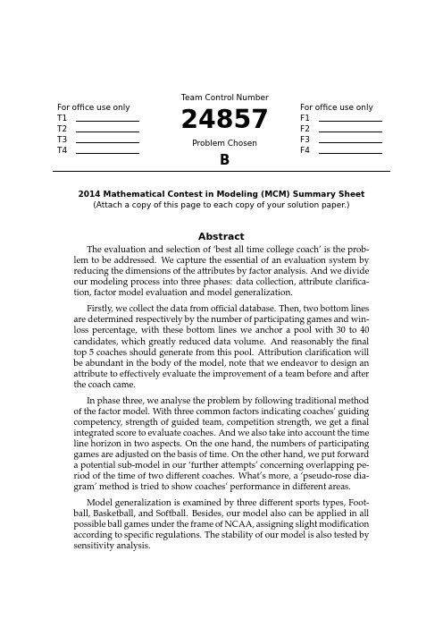
For office use only T1T2T3T4T eam Control Number24857Problem ChosenBFor office use onlyF1F2F3F42014Mathematical Contest in Modeling(MCM)Summary Sheet (Attach a copy of this page to each copy of your solution paper.)AbstractThe evaluation and selection of‘best all time college coach’is the prob-lem to be addressed.We capture the essential of an evaluation system by reducing the dimensions of the attributes by factor analysis.And we divide our modeling process into three phases:data collection,attribute clarifica-tion,factor model evaluation and model generalization.Firstly,we collect the data from official database.Then,two bottom lines are determined respectively by the number of participating games and win-loss percentage,with these bottom lines we anchor a pool with30to40 candidates,which greatly reduced data volume.And reasonably thefinal top5coaches should generate from this pool.Attribution clarification will be abundant in the body of the model,note that we endeavor to design an attribute to effectively evaluate the improvement of a team before and after the coach came.In phase three,we analyse the problem by following traditional method of the factor model.With three common factors indicating coaches’guiding competency,strength of guided team,competition strength,we get afinal integrated score to evaluate coaches.And we also take into account the time line horizon in two aspects.On the one hand,the numbers of participating games are adjusted on the basis of time.On the other hand,we put forward a potential sub-model in our‘further attempts’concerning overlapping pe-riod of the time of two different coaches.What’s more,a‘pseudo-rose dia-gram’method is tried to show coaches’performance in different areas.Model generalization is examined by three different sports types,Foot-ball,Basketball,and Softball.Besides,our model also can be applied in all possible ball games under the frame of NCAA,assigning slight modification according to specific regulations.The stability of our model is also tested by sensitivity analysis.Who’s who in College Coaching Legends—–A generalized Factor Analysis approach2Contents1Introduction41.1Restatement of the problem (4)1.2NCAA Background and its coaches (4)1.3Previous models (4)2Assumptions5 3Analysis of the Problem5 4Thefirst round of sample selection6 5Attributes for evaluating coaches86Factor analysis model106.1A brief introduction to factor analysis (10)6.2Steps of Factor analysis by SPSS (12)6.3Result of the model (14)7Model generalization15 8Sensitivity analysis189Strength and Weaknesses199.1Strengths (19)9.2Weaknesses (19)10Further attempts20 Appendices22 Appendix A An article for Sports Illustrated221Introduction1.1Restatement of the problemThe‘best all time college coach’is to be selected by Sports Illustrated,a magazine for sports enthusiasts.This is an open-ended problem—-no limitation in method of performance appraisal,gender,or sports types.The following research points should be noted:•whether the time line horizon that we use in our analysis make a difference;•the metrics for assessment are to be articulated;•discuss how the model can be applied in general across both genders and all possible sports;•we need to present our model’s Top5coaches in each of3different sports.1.2NCAA Background and its coachesNational Collegiate Athletic Association(NCAA),an association of1281institution-s,conferences,organizations,and individuals that organizes the athletic programs of many colleges and universities in the United States and Canada.1In our model,only coaches in NCAA are considered and ranked.So,why evaluate the Coaching performance?As the identity of a college football program is shaped by its head coach.Given their impacts,it’s no wonder high profile athletic departments are shelling out millions of dollars per season for the services of coaches.Nick Saban’s2013total pay was$5,395,852and in the same year Coach K earned$7,233,976in total23.Indeed,every athletic director wants to hire the next legendary coach.1.3Previous modelsTraditionally,evaluation in athletics has been based on the single criterion of wins and losses.Years later,in order to reasonably evaluate coaches,many reseachers have implemented the coaching evaluation model.Such as7criteria proposed by Adams:[1] (1)the coach in the profession,(2)knowledge of and practice of medical aspects of coaching,(3)the coach as a person,(4)the coach as an organizer and administrator,(5) knowledge of the sport,(6)public relations,and(7)application of kinesiological and physiological principles.1Wikipedia:/wiki/National_Collegiate_Athletic_ Association#NCAA_sponsored_sports2USAToday:/sports/college/salaries/ncaaf/coach/ 3USAToday:/sports/college/salaries/ncaab/coach/Such models relatively focused more on some subjective and difficult-to-quantify attributes to evaluate coaches,which is quite hard for sports fans to judge coaches. Therefore,we established an objective and quantified model to make a list of‘best all time college coach’.2Assumptions•The sample for our model is restricted within the scale of NCAA sports.That is to say,the coaches we discuss refers to those service for NCAA alone;•We do not take into account the talent born varying from one player to another, in this case,we mean the teams’wins or losses purely associate with the coach;•The difference of games between different Divisions in NCAA is ignored;•Take no account of the errors/amendments of the NCAA game records.3Analysis of the ProblemOur main goal is to build and analyze a mathematical model to choose the‘best all time college coach’for the previous century,i.e.from1913to2013.Objectively,it requires numerous attributes to judge and specify whether a coach is‘the best’,while many of the indicators are deemed hard to quantify.However,to put it in thefirst place, we consider a‘best coach’is,and supposed to be in line with several basic condition-s,which are the prerequisites.Those prerequisites incorporate attributes such as the number of games the coach has participated ever and the win-loss percentage of the total.For instance,under the conditions that either the number of participating games is below100,or the win-loss percentage is less than0.5,we assume this coach cannot be credited as the‘best’,ignoring his/her other facets.Therefore,an attempt was made to screen out the coaches we want,thus to narrow the range in ourfirst stage.At the very beginning,we ignore those whose guiding ses-sions or win-loss percentage is less than a certain level,and then we determine a can-didate pool for‘the best coach’of30-40in scale,according to merely two indicators—-participating games and win-loss percentage.It should be reasonably reliable to draw the top5best coaches from this candidate pool,regardless of any other aspects.One point worth mentioning is that,we take time line horizon as one of the inputs because the number of participating games is changing all the time in the previous century.Hence,it would be unfair to treat this problem by using absolute values, especially for those coaches who lived in the earlier ages when sports were less popular and games were sparse comparatively.4Thefirst round of sample selectionCollege Football is thefirst item in our research.We obtain data concerning all possible coaches since it was initiated,of which the coaches’tenures,participating games and win-loss percentage etc.are included.As a result,we get a sample of2053in scale.Thefirst10candidates’respective information is as below:Table1:Thefirst10candidates’information,here Pct means win-loss percentageCoach From To Years Games Wins Losses Ties PctEli Abbott19021902184400.5Earl Abell19281930328141220.536Earl Able1923192421810620.611 George Adams1890189233634200.944Hobbs Adams1940194632742120.185Steve Addazio20112013337201700.541Alex Agase1964197613135508320.378Phil Ahwesh19491949193600.333Jim Aiken19461950550282200.56Fred Akers19751990161861087530.589 ...........................Firstly,we employ Excel to rule out those who begun their coaching career earlier than1913.Next,considering the impact of time line horizon mentioned in the problem statement,we import our raw data into MATLAB,with an attempt to calculate the coaches’average games every year versus time,as delineated in the Figure1below.Figure1:Diagram of the coaches’average sessions every year versus time It can be drawn from thefigure above,clearly,that the number of each coach’s average games is related with the participating time.With the passing of time and the increasing popularity of sports,coaches’participating games yearly ascends from8to 12or so,that is,the maximum exceed the minimum for50%around.To further refinethe evaluation method,we make the following adjustment for coaches’participating games,and we define it as each coach’s adjusted participating games.Gi =max(G i)G mi×G iWhere•G i is each coach’s participating games;•G im is the average participating games yearly in his/her career;and•max(G i)is the max value in previous century as coaches’average participating games yearlySubsequently,we output the adjusted data,and return it to the Excel table.Obviously,directly using all this data would cause our research a mass,and also the economy of description is hard to achieved.Logically,we propose to employ the following method to narrow the sample range.In general,the most essential attributes to evaluate a coach are his/her guiding ex-perience(which can be shown by participating games)and guiding results(shown by win-loss percentage).Fortunately,these two factors are the ones that can be quantified thus provide feasibility for our modeling.Based on our common sense and select-ed information from sports magazines and associated programs,wefind the winning coaches almost all bear the same characteristics—-at high level in both the partici-pating games and the win-loss percentage.Thus we may arbitrarily enact two bottom line for these two essential attributes,so as to nail down a pool of30to40candidates. Those who do not meet our prerequisites should not be credited as the best in any case.Logically,we expect the model to yield insight into how bottom lines are deter-mined.The matter is,sports types are varying thus the corresponding features are dif-ferent.However,it should be reasonably reliable to the sports fans and commentators’perceptual intuition.Take football as an example,win-loss percentage that exceeds0.75 should be viewed as rather high,and college football coaches of all time who meet this standard are specifically listed in Wikipedia.4Consequently,we are able tofix upon a rational pool of candidate according to those enacted bottom lines and meanwhile, may tender the conditions according to the total scale of the coaches.Still we use Football to further articulate,to determine a pool of candidates for the best coaches,wefirst plot thefigure below to present the distributions of all the coaches.From thefigure2,wefind that once the games number exceeds200or win-loss percentage exceeds0.7,the distribution of the coaches drops significantly.We can thus view this group of coaches as outstanding comparatively,meeting the prerequisites to be the best coaches.4Wikipedia:/wiki/List_of_college_football_coaches_ with_a_.750_winning_percentageFigure2:Hist of the football coaches’number of games versus and average games every year versus games and win-loss percentageHence,we nail down the bottom lines for both the games number and the win-loss percentage,that is,0.7for the former and200for the latter.And these two bottom lines are used as the measure for ourfirst round selection.After round one,merely35 coaches are qualified to remain in the pool of candidates.Since it’s thefirst round sifting,rather than direct and ultimate determination,we hence believe the subjectivity to some extent in the opt of bottom lines will not cloud thefinal results of the best coaches.5Attributes for evaluating coachesThen anchored upon the35candidate selected,we will elaborate our coach evaluation system based on8attributes.In the indicator-select process,we endeavor to examine tradeoffs among the availability for data and difficulty for data quantification.Coaches’pay,for example,though serves as the measure for coaching evaluation,the corre-sponding data are limited.Situations are similar for attributes such as the number of sportsmen the coach ever cultivated for the higher-level tournaments.Ultimately,we determine the8attributes shown in the table below:Further explanation:•Yrs:guiding years of a coach in his/her whole career•G’:Gi =max(G i)G mi×G i see it at last section•Pct:pct=wins+ties/2wins+losses+ties•SRS:a rating that takes into account average point differential and strength of schedule.The rating is denominated in points above/below average,where zeroTable2:symbols and attributessymbol attributeYrs yearsG’adjusted overall gamesPct win-lose percentageP’Adjusted percentage ratioSRS Simple Rating SystemSOS Strength of ScheduleBlp’adjusted Bowls participatedBlw’adjusted Bowls wonis the average.Note that,the bigger for this value,the stronger for the team performance.•SOS:a rating of strength of schedule.The rating is denominated in points above/below average,where zero is the average.Noted that the bigger for this value,the more powerful for the team’s rival,namely the competition is more fierce.Sports-reference provides official statistics for SRS and SOS.5•P’is a new attribute designed in our model.It is the result of Win-loss in the coach’s whole career divided by the average of win-loss percentage(weighted by the number of games in different colleges the coach ever in).We bear in mind that the function of a great coach is not merely manifested in the pure win-loss percentage of the team,it is even more crucial to consider the improvement of the team’s win-loss record with the coach’s participation,or say,the gap between‘af-ter’and‘before’period of this team.(between‘after’and‘before’the dividing line is the day the coach take office)It is because a coach who build a comparative-ly weak team into a much more competitive team would definitely receive more respect and honor from sports fans.To measure and specify this attribute,we col-lect the key official data from sports-reference,which included the independent win-loss percentage for each candidate and each college time when he/she was in the team and,the weighted average of all time win-loss percentage of all the college teams the coach ever in—-regardless of whether the coach is in the team or not.To articulate this attribute,here goes a simple physical example.Ike Armstrong (placedfirst when sorted by alphabetical order),of which the data can be ob-tained from website of sports-reference6.We can easily get the records we need, namely141wins,55losses,15ties,and0.704for win-losses percentage.Fur-ther,specific wins,losses,ties for the team he ever in(Utab college)can also be gained,respectively they are602,419,30,0.587.Consequently,the P’value of Ike Armstrong should be0.704/0.587=1.199,according to our definition.•Bowl games is a special event in thefield of Football games.In North America,a bowl game is one of a number of post-season college football games that are5sports-reference:/cfb/coaches/6sports-reference:/cfb/coaches/ike-armstrong-1.htmlprimarily played by teams from the Division I Football Bowl Subdivision.The times for one coach to eparticipate Bowl games are important indicators to eval-uate a coach.However,noted that the total number of Bowl games held each year is changing from year to year,which should be taken into consideration in the model.Other sports events such as NCAA basketball tournament is also ex-panding.For this reason,it is irrational to use the absolute value of the times for entering the Bowl games (or NCAA basketball tournament etc.)and the times for winning as the evaluation measurement.Whereas the development history and regulations for different sports items vary from one to another (actually the differentiation can be fairly large),we here are incapable to find a generalized method to eliminate this discrepancy ,instead,in-dependent method for each item provide a way out.Due to the time limitation for our research and the need of model generalization,we here only do root extract of blp and blw to debilitate the differentiation,i.e.Blp =√Blp Blw =√Blw For different sports items,we use the same attributes,except Blp’and Blw’,we may change it according to specific sports.For instance,we can use CREG (Number of regular season conference championship won)and FF (Number of NCAA Final Four appearance)to replace Blp and Blw in basketball games.With all the attributes determined,we organized data and show them in the table 3:In addition,before forward analysis there is a need to preprocess the data,owing to the diverse dimensions between these indicators.Methods for data preprocessing are a lot,here we adopt standard score (Z score)method.In statistics,the standard score is the (signed)number of standard deviations an observation or datum is above the mean.Thus,a positive standard score represents a datum above the mean,while a negative standard score represents a datum below the mean.It is a dimensionless quantity obtained by subtracting the population mean from an individual raw score and then dividing the difference by the population standard deviation.7The standard score of a raw score x is:z =x −µσIt is easy to complete this process by statistical software SPSS.6Factor analysis model 6.1A brief introduction to factor analysisFactor analysis is a statistical method used to describe variability among observed,correlated variables in terms of a potentially lower number of unobserved variables called factors.For example,it is possible that variations in four observed variables mainly reflect the variations in two unobserved variables.Factor analysis searches for 7Wikipedia:/wiki/Standard_scoreTable3:summarized data for best college football coaches’candidatesCoach From To Yrs G’Pct Blp’Blw’P’SRS SOS Ike Armstrong19251949252810.70411 1.199 4.15-4.18 Dana Bible19151946313860.7152 1.73 1.0789.88 1.48 Bernie Bierman19251950242780.71110 1.29514.36 6.29 Red Blaik19341958252940.75900 1.28213.57 2.34 Bobby Bowden19702009405230.74 5.74 4.69 1.10314.25 4.62 Frank Broyles19571976202570.7 3.162 1.18813.29 5.59 Bear Bryant19451982385080.78 5.39 3.87 1.1816.77 6.12 Fritz Crisler19301947182080.76811 1.08317.15 6.67 Bob Devaney19571972162080.806 3.16 2.65 1.25513.13 2.28 Dan Devine19551980222800.742 3.16 2.65 1.22613.61 4.69 Gilmour Dobie19161938222370.70900 1.27.66-2.09 Bobby Dodd19451966222960.713 3.613 1.18414.25 6.6 Vince Dooley19641988253250.715 4.47 2.83 1.09714.537.12 Gus Dorais19221942192320.71910 1.2296-3.21 Pat Dye19741992192400.707 3.16 2.65 1.1929.68 1.51 LaVell Edwards19722000293920.716 4.69 2.65 1.2437.66-0.66 Phillip Fulmer19922008172150.743 3.87 2.83 1.08313.42 4.95 Woody Hayes19511978283290.761 3.32 2.24 1.03117.418.09 Frank Kush19581979222710.764 2.65 2.45 1.238.21-2.07 John McKay19601975162070.7493 2.45 1.05817.298.59 Bob Neyland19261952212860.829 2.65 1.41 1.20815.53 3.17 Tom Osborne19731997253340.8365 3.46 1.18119.7 5.49 Ara Parseghian19561974192250.71 2.24 1.73 1.15317.228.86 Joe Paterno19662011465950.749 6.08 4.9 1.08914.01 5.01 Darrell Royal19541976232970.7494 2.83 1.08916.457.09 Nick Saban19902013182390.748 3.74 2.83 1.12313.41 3.86 Bo Schembechler19631989273460.775 4.12 2.24 1.10414.86 3.37 Francis Schmidt19221942212670.70800 1.1928.490.16 Steve Spurrier19872013243160.733 4.363 1.29313.53 4.64 Bob Stoops19992013152070.804 3.74 2.65 1.11716.66 4.74 Jock Sutherland19191938202550.81221 1.37613.88 1.68 Barry Switzer19731988162090.837 3.61 2.83 1.16320.08 6.63 John Vaught19471973253210.745 4.24 3.16 1.33814.7 5.26 Wallace Wade19231950243070.765 2.24 1.41 1.34913.53 3.15 Bud Wilkinson19471963172220.826 2.83 2.45 1.14717.54 4.94 such joint variations in response to unobserved latent variables.The observed vari-ables are modelled as linear combinations of the potential factors,plus‘error’terms. The information gained about the interdependencies between observed variables can be used later to reduce the set of variables in a putationally this technique is equivalent to low rank approximation of the matrix of observed variables.8 Why carry out factor analyses?If we can summarise a multitude of measure-8Wikipedia:/wiki/Factor_analysisments with a smaller number of factors without losing too much information,we have achieved some economy of description,which is one of the goals of scientific investi-gation.It is also possible that factor analysis will allow us to test theories involving variables which are hard to measure directly.Finally,at a more prosaic level,factor analysis can help us establish that sets of questionnaire items(observed variables)are in fact all measuring the same underlying factor(perhaps with varying reliability)and so can be combined to form a more reliable measure of that factor.6.2Steps of Factor analysis by SPSSFirst we import the decided datasets of8attributes into SPSS,and the results can be obtained below after the software processing.[2-3]Figure3:Table of total variance explainedFigure4:Scree PlotThefirst table and scree plot shows the eigenvalues and the amount of variance explained by each successive factor.The remaining5factors have small eigenvalues value.Once the top3factors are extracted,it adds up to84.3%,meaning a great as the explanatory ability for the original information.To reflect the quantitative analysis of the model,we obtain the following factor loading matrix,actually the loadings are in corresponding to the weight(α1,α2 (i)the set ofx i=αi1f1+αi2f2+...+αim f j+εiAnd the relative strength of the common factors and the original attribute can also be manifested.Figure5:Rotated Component MatrixThen,with Rotated Component Matrix above,wefind the common factor F1main-ly expresses four attributes they are:G,Yrs,P,SRS,and logically,we define the com-mon factor generated from those four attributes as the guiding competency of the coach;similarly,the common factor F2mainly expresses two attributes,and they are: Pct and Blp,which can be de defined as the integrated strength of the guided team; while the common factor F3,mainly expresses two attributes:SOS and Blw,which can be summarized into a‘latent attribute’named competition strength.In order to obtain the quantitative relation,we get the following Component Score Coefficient Matrix processed by SPSS.Further,the function of common factors and the original attributes is listed as bel-low:F1=0.300x1+0.312x2+0.023x3+0.256x4+0.251x5+0.060x6−0.035x7−0.053x8F2=−0.107x1−0,054x2+0.572x3+0.103x4+0.081x5+0.280x6+0.372x7+0.142x8 F3=−0.076x1−0,098x2−0.349x3+0.004x4+0.027x5−0.656x6+0.160x7+0.400x8 Finally we calculate out the integrated factor scores,which should be the average score weighted by the corresponding proportion of variance contribution of each com-mon factor in the total variance contribution.And the function set should be:F=0.477F1+0.284F2+0.239F3Figure6:Component Score Coefficient Matrix6.3Result of the modelwe rank all the coaches in the candidate pool by integrated score represented by F.Seetable4:Table4:Integrated scores for best college football coach(show15data due to the limi-tation of space)Rank coaches F1F2F3Integrated factor1Joe Paterno 3.178-0.3150.421 1.3622Bobby Bowden 2.51-0.2810.502 1.1113Bear Bryant 2.1420.718-0.142 1.0994Tom Osborne0.623 1.969-0.2390.8205Woody Hayes0.140.009 1.6130.4846Barry Switzer-0.705 2.0360.2470.4037Darrell Royal0.0460.161 1.2680.4018Vince Dooley0.361-0.442 1.3730.3749Bo Schembechler0.4810.1430.3040.32910John Vaught0.6060.748-0.870.26511Steve Spurrier0.5180.326-0.5380.18212Bob Stoops-0.718 1.0850.5230.17113Bud Wilkinson-0.718 1.4130.1050.16514Bobby Dodd0.08-0.2080.7390.16215John McKay-0.9620.228 1.870.151Based on this model,we can make a scientific rank list for US college football coach-es,the Top5coaches of our model is Joe Paterno,Bobby Bowden,Bear Bryant,TomOsborne,Woody Hayes.In order to confirm our result,we get a official list of bestcollege football coaches from Bleacherreport99Bleacherreport:/articles/890705-college-football-the-top-50-coTable5:The result of our model in football,the last column is official college basketball ranking from bleacherreportRank Our model Integrated scores bleacherreport1Joe Paterno 1.362Bear Bryant2Bobby Bowden 1.111Knute Rockne3Bear Bryant 1.099Tom Osborne4Tom Osborne0.820Joe Paterno5Woody Hayes0.484Bobby Bowden By comparing thoes two ranking list,wefind that four of our Top5coaches ap-peared in the offical Top5list,which shows that our model is reasonable and effective.7Model generalizationOur coach evaluation system model,of which the feasibility of generalization is sat-isfying,can be accommodated to any possible NCAA sports concourses by assigning slight modification concerning specific regulations.Besides,this method has nothing to do with the coach’s gender,or say,both male and female coaches can be rationally evaluated by this system.And therefore we would like to generalize this model into softball.Further,we take into account the time line horizon,making corresponding adjust-ment for the indicator of number of participating games so as to stipulate that the evaluation measure for1913and2013would be the same.To further generalize the model,first let’s have a test in basketball,of which the data available is adequate enough as football.And the specific steps are as following:1.Obtain data from sports-reference10and rule out the coaches who begun theircoaching career earlier than1913.2.Calculate each coach’s adjusted number of participating games,and adjust theattribute—-FF(Number of NCAA Final Four appearance).3.Determine the bottom lines for thefirst round selection to get a pool of candidatesaccording to the coaches’participating games and win-loss percentage,and the ideal volumn of the pool should be from30to40.Hist diagrams are as below: We determine800as the bottom line for the adjusted participating games and0.7 for the win-loss percentage.Coincidently,we get a candidate pool of35in scale.4.Next,we collect the corresponding data of candidate coaches(P’,SRS,SOS etc.),as presented in the table6:5.Processed by z score method and factor analysis based on the8attributes anddata above,we get three common factors andfinal integrated scores.And among 10sports-reference:/cbb/coaches/Figure7:Hist of the basketball coaches’number of games versus and average gamesevery year versus games and win-loss percentagethe top5candidates,Mike Krzyzewski,Adolph Rupp,Dean SmithˇcˇnBob Knightare the same with the official statistics from bleacherreport.11We can say theeffectiveness of the model is pretty good.See table5.We also apply similar approach into college softball.Maybe it is because the popularity of the softball is not that high,the data avail-able is not adequate to employ ourfirst model.How can our model function in suchsituation?First and foremost,specialized magazines like Sports Illustrated,its com-mentators there would have more internal and confidential databases,which are notexposed publicly.On the one hand,as long as the data is adequate enough,we can saythe original model is completely feasible.While under the situation that there is datadeficit,we can reasonably simplify the model.The derivation of the softball data is NCAA’s official websites,here we only extractdata from All-Division part.12Softball is a comparatively young sports,hence we may arbitrarily neglect the re-stricted condition of‘100years’.Subsequently,because of the data deficit it is hard toadjust the number of participating games.We may as well determine10as the bottomline for participating games and0.74for win-loss percentage,producing a candidatepool of33in scaleAttributed to the inadequacy of the data for attributes,it is not convenient to furtheruse the factor analysis similarly as the assessment model.Therefore,here we employsolely two of the most important attributes to evaluate a coach and they are:partic-ipating games and win-loss percentage in the coach’s whole career.Specifically,wefirst adopt z score to normalize all the data because of the differentiation of various dimensions,and then the integrated score of the coach can be reached by the weighted11bleacherreport:/articles/1341064-10-greatest-coaches-in-ncaa-b 12NCAA softball Coaching Record:/Docs/stats/SB_Records/2012/coaches.pdf。
2014年美赛数模B题-Finalist

24270 T4 ________________ F4 ________________Team Control NumberFor office use only For office use only T1 ________________ F1 ________________ T2 ________________ F2 ________________ T3 ________________ F3 ________________ Problem Chosen B2014 Mathematical Contest in Modeling (MCM) Summary SheetSummaryIn order to estimate the excellence of different sports coaches and to give a ranking result, two distinct models are developed. The first model is a comprehensive evaluation method. And the second model is a ranking algorithm analogous to the Journal Influence Algorithm . In the first model, we take into account a variety of metrics, and divide them into twocategories: Objective Metrics and Subjective Metrics . In the Objective Metrics , we consider four factors, the number of wins, winning percentage, champions and final fours. All these factors have contributions to the excellence of a coach. We deem that the total number of games in a year could affect the number of wins, and the unevenness of team quality could affect the winning percentage. By employing statistical regression method to process collected data, we establish two functions of influence coefficient to eliminate thediscrepancy caused by the two kinds of effect. In the Subjective Metrics : we consider two factors, media popularity and tenure. We employ Fuzzy Analysis Method to quantify these two subjective factors. We further incorporate Analytic Hierarchy Process (AHP) and Gray Relational Analysis Grade Method (GRAP) to determine the weight allocation to different metrics. The final ranking gives a comprehensive result by weighing results returned by these two methods. Using data from Sports Reference and other websites, the rankings in basketball, football and baseball accord with previous media commentaries.In the second model, we deem that the excellence of a certain coach can be reflected from the media impact over the span of history and that the interactions between two coaches can reflect the disparity of skill level between them. We use search results returned by Google to quantify the impact of one coach on another. Based on the search results, we build a cross-reference matrix to represent relationships between coaches. In view that the different time periods that two coaches were in may largely affect the interaction between them, and the personal reputation may influence the number of search results, we develop a weight function of two variables to compensate the influence of time and to rule out the redundant information.In consideration of the similarity between personal influence and journal influence, we refer to the Journal Influence Algorithm introduced by Eigenfactor and establish a new ranking algorithm. The basic idea of the algorithm is subtle: using weight function to modify the cross-reference matrix , and taking into consideration of individual influence, the algorithm gives an evaluation vector to rank different coaches. To test the validity of this algorithm, we apply the algorithm into basketball, football and baseball. The algorithm gives a result that is similar to the result obtained in the first model. The ranking also agrees withprevious media commentaries. Furthermore, by slightly adjusting the coefficients, we can apply the algorithm into various sports.“Dream Team” of College Coaches# Team 24270Team # 24270 Page 2 of 26Contents1. Introduction (3)1.1. Restatement of the Problem (3)1.2. Model Overview (3)2. Assumptions (3)3. ModelⅠ (4)3.1. Additional assumptions (4)3.2. Notations (4)3.3. Evaluation System (5)3.3.1. The influence of time on the total number of wins (6)3.3.2. The influence of time on the winning-percentage (6)3.3.3. Fuzzy Analysis (7)3.3.4. Nondimensionalization process (8)3.3.5. Final result (8)3.4. Solutions to ModelⅠ (10)3.4.1. Basketball (10)3.4.2. Football (11)3.4.3. Baseball (12)3.4.4. Sensitivity analysis (13)4. ModelⅡ (13)4.1. Additional assumptions (14)4.2. Notations (14)4.3. The Individual Influence Vector (14)4.3.1. Original data (15)4.3.2. The influence coefficient of time (15)4.3.3. The influence coefficient of reputation (16)4.3.3. The individual influence vector (16)4.4. The Cross-Reference Matrix (16)4.4.1. The weight function (17)4.4.2. The final cross-reference matrix (17)4.5. The Evaluation Vector (18)4.6. Solutions to Model II (18)4.6.1. Basketball (18)4.6.2. Football (19)4.6.3. Baseball (19)4.6.4. Sensitivity analysis (19)5. Applicability (20)6. Strengths and Limitations (21)6.1. ModelⅠ (21)6.2. Model II (21)7. Conclusions (21)8. The Article for Sports Illustrated (22)References (23)Appendix (24)Team # 24270 Page 3 of 261. Introduction1.1. Restatement of the ProblemSports, by definition, is all forms of usually competitive physical activity which aim to usephysical ability while providing entertainment to participants and spectators [1]. No wonder theword “sports” gives us a first impression of fierce competition, agitated spectators, sweating on the running track, combined with a joy of victory. It is the uncertainty that makes the sports game so intriguing. However, where there is competition, there will always be victory, defeat, and ranking. Loyal sport fans could debate day and night over the question who is thebest player or coach. These debates have called forth a need for certain criterion of sports coaches and players. The criterion has to be: (1) all-encompassing to take into consideration a variety of factors; (2) applicable to various sports; (3) robust enough to remain unaffected by fluctuation.1.2. Model Overview● Model Ⅰ The evaluation method in Model Ⅰis based on a comprehensive method sophistically combining Analytic Hierarchy Process(AHP) and Gray Relational Analysis GradeMethod(GRAP). In the evaluation process, we take into consideration the influence of time horizon, and incorporate Fuzzy Analysis Method, which make it feasible to compare diverse factors on the same level. The ranking results in three different sports accord with previous media report, which attest the validity of this method.● Model ⅡIn model II, we assume that the excellence of a certain coach can be reflected from the media impact over the span of history and thus can be gauged by the impact on another coach within or without the same period of time. We use Google search results to quantify the impact of one coach on another. The relationship between coaches can be established as a cross-reference matrix. By further taking into account the influence of time, influence of reputation, and a modification to rule out the redundant information, we obtain a finalevaluation vector. The final ranking result is roughly approximate to the result in model I. To sum up, we only need the search results returned by Google search engine to estimate the excellence of certain coach with high accuracy.2. Assumptions● We assume that the competition rules of each sport do not change.Although sports are developing, we do not take into account of time in the competition rules in order to compare the coaches of different years more fairly.● We neglect tied competitions since they have the same effect on the two comparedteams.● We only take the Division I into consideration.x , x , x ’’, x *Evaluation index matrix Team # 24270 Page 4 of 26Competitions are divided into three parts: Division I, II and III according to the level of sport strengths of different colleges. Since Division I always concludes top coaches, we only take Division I into consideration.● The selected data are valid.● Additional assumptions are made to simplify analysis for individual sections. Theseassumptions will be discussed at the appropriate sections.3. Model Ⅰ3.1. Additional assumptions● The evaluation system includes two parts: Objective Metrics(OM) and SubjectiveMetrics (SM).● We assume that OM include four specific indexes: the total number of wins, the winning-percentage, the number of final fours and the number of champions.● Tenure and media popularity are considered in SM.In the subjective metrics of ranking coaches, some factors are hard to investigate qualitatively and quantitatively due to lacking data, such as, his or her influence to players, range of knowledge, studying ability, team spirits, searching talents, acting in competitions, salary and so on. Therefore, we neglect these indexes in SM.● Time only makes a difference in the total number of wins, and the winningpercentage.In fact, the numbers of final fours and champions have no effect on the other two in OM, since the number of teams which are able to enter into final fours and even achievechampions is fixed. And we neglect the influence of time on media popularity in order to simplify the model.3.2. NotationsTable 1: Notations and DescriptionsNotations DescriptionsS i Evaluation objectx j Evaluation indexn The number of evaluation objectsm The number of evaluation indexes’ t Timep i , q i Influence coefficients of timeW (t ) The total number of competitions in ts (t ) The standard deviation of all winning-percentage in tM j Maximum of x ijm j Minimum of x ij, Grey relational coefficient ∆�� Absolute difference [ ] ( )1 2, , m x x =x . , 1x m >[ ]= 1 2 3 4 5 6x x , , , , ,x x x x x Team # 24270 Page 5 of 26 Notations Descriptionsf (x ) Subordinate functionA Pairwise comparison matrixλ The largest eigenvaluew Weight vectorCI Consistency indexRI Random consistency indexCR Consistency ratioB Evaluation vector of AHP (0)���Δmin Minimum differenceΔmax Maximum differencer Relation degree vectorC Evaluation vector of Grey Relation Degreeα , β Partial coefficientU Ultimate evaluation vector3.3. Evaluation SystemWe define n as the number of evaluation objects, and S 1, S 2,…, S n (n >1) are the evaluation objects. m is the number of evaluation indexes, and x 1, x 2,…, x m are the evaluation indexes. Evaluation index vector isTThe total evaluation indexes include OM: the total number of wins, the winning-percentage(pct.), the number of final fours and the number of champions and SM: tenure and media popularity. So m = 6 ,TWhere: ● x 1 — the total number of wins vector.● x 2 — the winning-percentage vector.● x 3 — the number of final fours vector.● x 4 — the number of champions vector.● x 5 — tenure vector.● x 6 — media popularity vector.i p = ' Team # 24270 Page 6 of 26 Figure 1: Flow chart of model I Undoubtedly, time plays an important role in evaluating top coaches. According to the assumptions, time only makes a difference in the total number of wins, the winning- percentage.3.3.1. The influence of time on the total number of winsWith the development of sports, the competition is getting relatively fiercer than ever, which means the disparity between teams become wider. The total number of games also increases with time going on. Therefore, when evaluating coaches in the previous century, the later certain coach begin his coaching career, the more likely he will get more wins. So we should put less weight on the coaches active in a later time period. And we can get a fairer evaluation of coaches within different time periods.In order to compensate the influence of t , we establish Influence Coefficients of Time (ICT) p i (i = 1,2, , n ) . We assume that the total number of competitions in t is W (t ) . W (t ) canbe obtained by statistical regression and simulating and curve fitting of selected data. So we define:1 W (t mi )where t mi is the middle year of tenure of S i . And then x 1i = x 1i ⋅ p i (i = 1,2, , n ) .3.3.2. The influence of time on the winning-percentageAs for the winning-percentage, sports were underdeveloped at an earlier time, and the quality disparity between teams is comparatively narrow. Therefore, the standard deviation of winning-percentage of each coach is closer to zero. Thus we should put less weight on the coaches active in a “mediocre” time period. We define ICT here as q i (i=1,2,…,n ), we assume that the standard deviation of all winning-percentage in t is s (t ) . s (t ) can be obtained by statistical regression and simulating and curve fitting of selected data. So we define:i q = ,1 3x ⎤ ≤ ≤⎪⎣ ⎦( ) 121 a x b --⎧⎡ + - ,1 3x ⎤ ≤ ≤⎪⎣ ⎦ ( ) 121 2.8049 0.4417x --⎧⎡ + - ' Team # 24270 Page 7 of 261 s (t mi )and x 2i = x 2i ⋅ q i (i = 1,2, , n ) .3.3.3. Fuzzy AnalysisAs for SM indexes, we assume that they can be divided into five levels: “ Excellent, Very Good, Good, Not Good, Bad”. And we correspond the five levels into 5,4,3,2,1 successively For continuous quantification, we assume:As for “Excellent”, we suppose f (5) = 1.As for “Very Good”, f (3) = 0.7 .As for “Bad”, f (1) = 0.1 .We employ partial large Cauchy distribution and the logarithmic function as the subordinate function [2]: f (x ) = ⎨⎩⎪c ln x + d , 3 ≤ x ≤ 5where a , b , c , d stands for undetermined constants. We use the initial conditions above to define their values. And solution of the subordinate function( Figure 2) is:f ( x ) = ⎨ (1) ⎪⎩0.5873ln x + 0.0548, 3 ≤ x ≤ 5Figure 2: Trend of f (x )Media popularity is measured by the number of search results via Google. The impact of duplication of names can be neglected by means of adding search keywords in order to rule out the redundant information.We map x j ( j =5,6) into interval [1,5], through function (1),we can obtain:( )4 ji j x m ⎛ ⎫-1x f ⎪=+()12 5,6i n j == (2)⎝ ⎭ =( )1, 2, ,6j =and ' ' ' ' '1 2 3, , , , j j j j n x x x x ⎡ ⎤= ⎣ ⎦x , , , , ,⎡ ⎤= ⎣ ⎦* '' '' '' '' '' ''1 2 3 4 5 6x x x x x x x(4) 1⎢ 2 ⎥⎢ ⎥1⎢ 5 3 ⎥1 3⎢ 5 3 ⎥3 1 5⎢ 3 ⎥⎥⎢ 2⎢ 3 1 ⎥⎥[ ]0.1248,0.1469,0.4593,0.8125,0.0775,0.2928=w 1≤ ≤1≤i ≤ n 1≤ ≤1≤i ≤ n ⎣ Team # 24270 Page 8 of 26M j - m j ⎪where M j = max {x ij } , m j = min {x ij} ( j = 5,6) .As for x 3 and x 4, we define that x 3’= x 3, x 4’= x 4.we use x 'j ( j = 1, 2, ,6) to proceed the following calculation.3.3.4. Nondimensionalization processWe employ extreme difference method to nondimensionalize the different indexes so that we can compare them [2]on the same level. The method is as follows:x 'ji - m jM j - m jTwhere M j = max {x ij } , m j = min {x ij } ( j = 1, 2, ,6) .and then we obtain the final evaluation index matrix:T3.3.5. Final resultBy using AHP as the subjective evaluation method and GRAP as the objective method, the final represents a comprehensive evaluation combined the merits of these two methods. Analytic Hierarchy Process [3] (AHP)By comparing the effect of two indexes x 'j ,the weights of the two method w ( x 'j )(j =1,2,…,m )are given. Then we construct the pairwise comparison matrix A .1 53 7 1 1⎢ 3 5 ⎥ 1A =⎢ 6 ⎥ ⎢ ⎥15 5 7 1 1 1 ⎢ 3 3 5 ⎦ We can obtain the largest eigenvalue of A :λ=6.0496 and its weight vector :Tn λ - CR = 0.008 0.1= <()(){ }( )1,2, ,x i n = =x( ) ( ) ( )ji i r x x = m m ρ∆ +∆( )0 max ji ρ∆ + ∆(ji i i x ∆ x = - ● —absolute difference.( )min min min i ∆ = ∆ —minimum difference of all indexes data.● ( )max max max i ∆ = ∆ —maximum difference of all indexes data.● 1w =∑(i i i w x = ∑ ( ) (,j r r x x = )j ( ) ,r x )j(6) Team # 24270 Page 9 of 26 After that, we must check the consistency of matrix A . The consistency index is calculated as follows:CI = = 9.92 ⨯10-3n -1From Table 2, the random consistency index RI =1.24Table 2: The Quantitative Values of RI [2]n 1 2 3 4 5 6 7 8 9 10 11 RI 0 0 0.58 0.90 1.12 1.24 1.32 1.41 1.45 1.49 1.51 Then, we can obtain consistency ratio: CIRI Therefore, we can safely draw the conclusion that the inconsistent degree of matrix A is in a tolerable range, and we can take its eigenvector as weight vector w [3].We define B as the evaluation vector of AHP, and B can be calculated as follows:B = x ' ⋅ w (5)In evaluation vector, the greater B i is, the higher ranking S i is.● Gray Relational Analysis Grade Method [4] (GRAP)We use integral grey relational degree to analyze the metrics data. And we take the total number of wins as the reference sequence:0 0and then we can obtain the gray relational coefficient [4]:, i = 1, 2, , n , j = 1,2, ,6Where:(0) (0)j ) jj i jj i ● ρ —resolution ration.For every coach S i , we determine its weight as w i , which should satisfy the requirements:n0 ≤ w i ≤ 1, ii =1 After determining the weight, we can obtain the relational degree [4]:ni =1And then we construct the relation degree vector [ ]1 2 3 4 5 6r r r = , where 1 1r = . , , , , ,r r r rTWe define C as the evaluation vector of AHP, and C can be calculated as follows::C = x ' ⋅ w (7)In evaluation vector, the greater C i is, the higher ranking S i is.● Combination of AHP and GRAPAt first, we employ extreme difference method to nondimensionalize the two evaluation vector B and C . And then, we construct an ultimate evaluation vector: U = α B + β C (8) where α , β respectively stands for the weight of AHP and GRAP, which should satisfy the requirements of α + β =1. Finally, we sort the value of U i (i =1,2,…,n ), and S i that corresponds to the top 5 of U i are top five coaches. 3.4. Solutions to Model ⅠWe choose three sports to verify our model and get the results, which include basketball, football and baseball.3.4.1. Basketball● Searching and selecting data We search and select data through the Internet [5][6][7]. For example, first, we search 100 coaches and their evaluation index data. Secondly, we rank them by comprehensively considering the total number of wins and the winning-percentage, so we can get top 40coaches. And then, we consider other metrics and rank top 20 coaches. Finally, the evaluation system is based on the selected 20 data. Table A1 in Appendix show the selected coaches and their evaluation index data.● Determining the final evaluation index matrixAt first, we determine vector x ’. For x 1, via the data in Table A2, we use W (t i )=Num 2, where Num represents the total number of teams in t i . We utilize software MATLAB to plot the graph of W (1)(t ) by simulating and curve fitting of data (Figure 3). So we can get p i for each S i , and then we obtain the vector x 1’.Figure 3: Trend of W (1)(x ) Figure 4: Trend of s (1)(x ) For x 2, via the data in Table A3, we also plot the graph of s (1)(t ) by simulating and curve fitting of data (Figure 4). So we can get q i for each S i , and then we obtain the vector x 2’.感谢作者分享]0.130 0.318 0.243 0, , , .482,1.761,0.138( ) [ ]19,14,8,12,9,7,18,11,3,5,16,10,1,2,17,4,13,6,20,15=1Rank ]1.000 0.316 0.151 0, , , .047, 0.392,0.052 For x 5 and x 4, from (1)(2), we can obtain x 5’ and x 6’.Secondly, from (3), we can obtain x ''j ( j = 1,2, ,6) . Finally, from (4), we can obtain x * .We list the quantitative value of x * in Table A4.● Obtaining the result via ultimate evaluation vectorAt first, from (5), we use AHP and get B . Secondly, we use GRAP and define that ρ=0.3and w i =0.05(i =1,2,…,n ). From (6), we can get the relation degree vector r . And then, from (7), we can obtain C . Finally, from (8), by defining α = 0.6, β = 0.4 , we can obtain the ultimate evaluation vector:U = [0.293,0.288,0.468,0.241,0.422,0.160,0.521,0.868,0.713,0.311,0.481,0.836,0.168,0.998, TBy sorting the value of U i (i =1,2,…,n ), we can obtain the ranking result of S i . And the ranking vector is: TTherefore, we list top five coaches of basketball in the previous century in Table 3:Table 3: Top 5 Coaches of Basketball No.1 No.2 No.3 No.4 No.5S 19 S 14 S 8 S 12 S 9John Wooden Dean Smith Mike Krzyzewski Adolph Rupp Bob KnightThis result is largely agreement with the widely accepted result [8][9].3.4.2. Football● Searching and selecting dataLike what we do in basketball, we search and select data through the Internet [5][10][11]. However, we calculate that the number of final fours is the sum number of times that teams can enter into Super Bowl.● Determining the final evaluation index matrixAt first, we determine vector x ’. For x 1, we use W (t i )=Num 2, where Num represents the total number of teams in t i .We can obtain W (2)(t ) by simulating and curve fitting of data. So we can get p i for each S i , and then we obtain the vector x 1’.For x 2, we also obtain s (1)(t ) by simulating and curve fitting of data. So we can get q i and the vector x 2’.Finally, from (4), we can obtain x * . We list the quantitative value of x * .● Obtaining the result via ultimate evaluation vectorLike what we do in Basketball, we can obtain the ultimate evaluation vector:U = [0.234,0.879,0.738,0.106,0.359,0.296,0.383,0.193,0.291,0.453,0.494,0.248,0.180,0.615,TBy sorting the value of U i (i =1,2,…,n ), we can obtain the ranking result of S i . And the ranking vector is: 感谢作者分享( ) [ ],2,3, ,11,10, ,7,5,16, ,9,12,1,8,1315 14 1 ,17,49 6 ,20,18=2Rank ''m t = 5t + ]0.022,0.044,0.232,0.225, 0.138,0.118( ) [ ],3,10,1,9,6, 2,17,18, 4,13,7,5,11,8,19, 20,161 ,12 ,15 4=3RankTTherefore, we list top five coaches of basketball in the previous century in Table 4:Table 4: Top 5 Coaches of Football No.1 No.2 No.3 No.4 No.5S 15 S 2 S 3 S 14 S 11 Joe Paterno Bobby Bowden Bear Bryant Tom Osborne Don JamesThis result is largely agreement with the widely accepted result [12].3.4.3. Baseball● Searching and selecting dataLike what we do in basketball, we search and select data through the Internet [13][14]. But in this sport, we assume that the number of final fours is the number of champions of NCAA competitions that teams can achieve. And we assume that the number of champions is the number of champions of National competitions that teams can get.● Determining the final evaluation index matrixAt first, we determine x ’. For x 1, due to scarcity of the data, we can only search a little information of several years [9]. We use W (t i )=Num 2, where Num represents the total number of competitions of champion in t i .We can obtain W (3)(t ) by simulating and curve fitting of data. So we can get p i for each S i , and then we obtain the vector x 1’.For x 2, due to lacking the standard difference of winning-percentage in every ten year, we choose another approach to get x 2’. Considering the influence of time, first, we employ extreme difference method to nondimensionalize t m into t m’, where t mi is the middle year of tenure of S i . Then, we define1'mand then we define x 2' i = x 2i ⋅ t mi '' . So from (3), we obtain x ''2 .Finally, from (4), we can obtain x *. We list the quantitative value of x *.● Obtaining the result via ultimate evaluation vectorLike what we do in Basketball, we can obtain the ultimate evaluation vector:U = [0.353,0.278,0.587,0.223,0.205,0.302,0.208,0.189,0.314,0.494,0.203,1.000,0.214,0,TBy sorting the value of U i (i =1,2,…,n ), we can obtain the ranking result of S i . And the ranking vector is:TTherefore, we list top five coaches of basketball in the previous century in Table 5:Table 5: Top 5 Coaches of Baseball感谢作者分享Team # 24270 Page 13 of 26No.1 No.2 No.3 No.4 No.5S15S2S3S14S11 John Barry Mike Martin Rod Dedeaux Augie Garrido Jim MorrisThis result is largely agreement with the widely accepted result[15].3.4.4. Sensitivity analysisBy changing the weight of AHP and GRAP in equation (8), we analyze the changing result of basketball. For example, we define α = 0.5, β = 0.5 , and the result is listed in Table 6.The coaches who rank top 5 do not change:Table 6: Top 5 Coaches of BasketballNo.1 No.2 No.3 No.4 No.5S19S12S14S8S9 John Wooden Adolph Rupp Dean Smith Mike Krzyzewski Bob KnightWhen defined α = 0.4, β = 0.6 , the result changes, which is listed in Table 7. The coaches who rank top five change:Table 7: Top 5 Coaches of BasketballNo.1 No.2 No.3 No.4 No.5S19S12S14S7S8 John Wooden Adolph Rupp Dean Smith Hank Iba Mike KrzyzewskiWhen defined α = 0.7, β = 0.3 , the result is listed in Table 8. The coaches who rank top five do not change:Table 8: Top 5 Coaches of BasketballNo.1 No.2 No.3 No.4 No.5S19S14S12S8S9 John Wooden Dean Smith Adolph Rupp Mike Krzyzewski Bob KnightAs can be seen from above, when there is a slight change of weights, the result do not change. But with a relatively greater change, weights have an effect on the result.4. ModelⅡHow could one’s reputation affect another’s? One way is to follow the implication in the saying: “You wouldn’t mention A and B in the same breath.” It means if the differencebetween two people is too wide, it would be unlikely for most of individuals to mention them in a same talk. The same holds true for the sports coaches. That means, if two coaches areabsolutely not on the same level, more likely than not, there will be few reports on these two coaches. On the other hand, if two of them are top coaches, there will be a plethora of reports: such as “The Greatest Coaches Ever” “Basketball Hall of Fame”, on the two coaches.Informed by this natural law, we may find an innovative approach to estimate a coach’s level of excellence and popularity. The working flow is shown as follows:感谢作者分享Team # 24270 Page 14 of 26Figure 5: Flow chart of model II4.1. Additional assumptions● The excellence of a coach and association between two coaches can be accuratelyreflected by the mass media.● The attention that the mass media have on certain coach is related to the search results onGoogle, in terms of number of pages, report orientation and report time.● The media attention is related to time and the excellence of certain coach. The influenceof time and excellence on the media attention remains unchanged to different kinds ofpeople.4.2. NotationsTable 9: Notations and DescriptionsNotations Descriptions��The number of search results of coach ik, b Coefficient of the function through linear regression��Characteristic year of coach iu The number of search results about sports careerICT Influence coefficient of timeICR Influence coefficient of reputationl Individual influence vectorZ Original cross-reference matrixWF Weight functionW Weighted cross-reference matrixα,βPartial coefficient4.3. The Individual Influence VectorBy our hypotheses, the excellence of a coach can be accurately reflected by the mass media.There are several ways to evaluate the media attention on a celebrity. One of the most simple and direct way is to record the number of search results on Google. However, the searchresults can be influenced by a variety of factors, such as time periods, tenure, etc. Bysimulating and curve fitting of sorted data, we evaluate the impact of such factors separately.Finally, we obtain a normalized individual influence vector.感谢作者分享( ) 1, 2, ,i n = (influence coefficient of time)=i ICT Team # 24270 Page 15 of 264.3.1. Original dataHere we define t i as the characteristic year , the average of the year that the coach i start coaching and the year of his or her retirement. (If the coach i is still active, then t is theaverage of the year that the coach i start coaching and this year, that is, 2014)The search results vector a is the original data we use to estimate the individual influence, where a i is the number of search results of coach i . Particularly, the coaches here are sorted bycharacteristic year in a descend order. This can be a great convenience to our later discussionabout time factor.4.3.2. The influence coefficient of timeAccording to the growth law of web information [16], the information aiming at a certainfield is similar to an exponent increase. To test this hypothesis and better apply it to sports, we entered the Google website. Using “1910 basketball”, “1920 basketball” , and “1930 basketball” as the “exact keywords”[17] respectively. The numbers of search results are shownin Table 10:Table 10: The Numbers of Search ResultsYear 1910 1920 1930 1940 1950 1960 1970 1980 1990 2000 2010Results 2750 5160 7440 11700 16200 26400 40200 25800 27000 67700 326000Assuming that this is an exponential function: y 1 = c ⋅ e dt . We use the least squared methodto obtain the unknown numbers in the function. See Figure 6.Figure 6: Trend of exponential function y 1 Figure 7: Trend of linear function y 2The result gives a satisfying simulation to the numbers of search results. However, thedistinction between 2000s and 1900s is too large. In our observation, the search results of coaches at different period of time is almost of the same magnitude of as each other. So, here we use the natural logarithm of the search results. Again we obtain a linear function y 2 as showed in Figure 7.The difference between maximum and minimum is about half of the minimum value. This is a modest value that we can safely put into use to estimate ICT . Common sense told us that the greater number of total reports is, the more “valuable” the search result is, the greater weight the search result will get. So, we define ICT as1 kt i + b 感谢作者分享。
2014数模美赛A
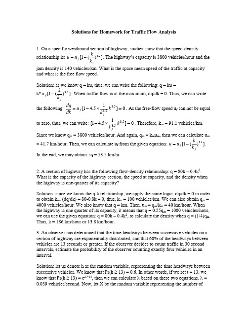
Solutions for Homework for Traffic Flow Analysis1. On a specific westbound section of highway, studies show that the speed-density relationship is: ])(1[5.3jf k k u u -=. The highway’s capacity is 3800 vehicles/hour and the jam density is 140 vehicles/km. What is the space mean speed of the traffic at capacity and what is the free flow speed.Solution: as we know q = ku, thus, we can write the following: q = ku = k*])(1[5.3jf k k u -. When traffic flow is at the maximum, dq/dk = 0. Thus, we can write the following: 0]15.41[5.35.3=⨯-=k k u dk dq jf . As the free-flow speed u f can not be equal to zero, thus, we can write: 0]15.41[5.35.3=⨯-k k j . Therefore, k m = 91.1 vehicles/km.Since we know q m = 3800 vehicles/hour. And again, q m = k m u m , then we can calculate u m= 41.7 km/hour. Then, we can calculate u f from the given equation: ])(1[5.3jf k k u u -=. In the end, we may obtain: u f = 53.5 km/hr.2. A section of highway has the following flow-density relationship: q = 80k – 0.4k 2. What is the capacity of the highway section, the speed at capacity, and the density when the highway is one-quarter of its capacity?Solution: since we know the q-k relationship, we apply the same logic: dq/dk = 0 in order to obtain k m . (dq/dk) = 80-0.8k = 0, thus, k m = 100 vehicles/km. We can also obtain q m = 4000 vehicles/hour. We also know that q = km. Then, u m = q m /k m = 40 km/hour. When the highway is one quarter of its capacity, it means that q = 0.25q m = 1000 vehicles/hour, we can use the given equation: q = 80k – 0.4k 2, to calculate the density when q = (1/4)q m . Thus, k = 186 km/hour or 13.8 km/hour.3. An observer has determined that the time headways between successive vehicles on a section of highway are exponentially distributed, and that 60% of the headways between vehicles are 13 seconds or greater. If the observer decides to count traffic in 30 second intervals, estimate the probability of the observer counting exactly four vehicles in an interval.Solution: let us denote h as the random variable, representing the time headways between successive vehicles. We know that Pr(h ≥ 13) = 0.6. In other words, if we set t = 13, we know that Pr(h ≥ 13) = e -λ*13, then we can calculate λ based on these two equations. λ = 0.039 vehicles/second. Now, let X be the random variable representing the number ofvehicle arrivals during time t, then X is poisson distributed. Pr(X=4) ==⨯=⨯--!4)30039.0(!)(30039.4e x e t t x λλ0.024.4. A vehicle pulls out onto a single-lane highway that has a flow rate of 280 vehicles/hour (poisson distributed). The driver of the vehicle does not look for oncoming traffic. Road conditions and vehicle speeds on the highway are such that it takes 1.5 seconds for an oncoming vehicle to stop once the brakes are applied. Assuming that a standard driver reaction time is 2.5 seconds, what is the probability that the vehicle pulling out will be in an accident with oncoming traffic?Solution: in this case, if the vehicle headways between successive vehicles are greater than 4 seconds, then the driver pulling out will not be in an accident. Or say, if the headways are less than 4 seconds, the driver pulling out will be in an accident.Since q = 280 vehicles/hour, then λ = 0.078 vehicles/second.Pr(h < 4) = 1-e -λt = 1-e -0.078*4 = 0.268.5. Reconsider the problem 4 above, how quick would the driver reaction times of oncoming vehicles have to be to have the probability of an accident equal to 0.15?Solution: let t denote the new driver reaction time. So,Pr[h < (1.5+t)] = 1 – e -0.078*(1.5+t) = 0.15, then, we can obtain t = 0.58.In other words, to reduce the probability of an accident to 0.15, the driver reaction must be less than 0.58 seconds.6. A toll booth on a turnpike is open from 8:00 am to 12 midnight. Vehicles start arriving at 7:45 am at a uniform deterministic rate of 6 per minute until 8:15 am and from then on at 2 per minute. If vehicles are processed at a uniform deterministic rate of 6 per minute, determine when the queue will dissipate, total delay, longest queue length (in vehicles), longest vehicle delay under first-in and first-out rule.Solutions: arrival rate λ1 = 6 vehicles/minute from 7:45 am to 8:15 am. λ2 = 2vehicles/minute from 8:15 am to the rest of the day. Departure rate μ = 2 vehicles/minute.Solution: the time when the queue will dissipate is then the arrival curve intersects with the departure curve. Q1 = 6t; Q2 = 120+2t; Q3 = -90 + 6t, where Q1 is the arrival curve between 7:45 am to 8 am and Q2 is the arrival curve starting from 8:15 am to the rest of the day and Q3 is the departure curve. By setting Q2 = Q3, we can obtain the value for t, the time when the queue dissipates, we obtain that t = 52.5 minutes. In other words, at 8:375 am, the queue completely dissipates.Because Q2 and Q3 are parallel to each other, the long delay happens anywhere on the Q1 curve and it is equal to 15 minutes. This means that every car arriving between 7:45 am to 8:15 am has to wait for 15 minutes in the queue. Also because Q2 and Q3 areparallel, the queue length is uniform between 7:45 am to 8:15 am too. The queue length is equal to 90 vehicles (Q1=6t = 6*15 = 90 vehicles).To calculate the total delay, we simply do the following:8 am 7:45 am 8:15 amTotal delay = ⎰+--⎰++⎰5.52155.5230300)690()2120(6dt t dt t tdt= 5.521525.523023002|)390(|)120(|3t t t t t +--++ = )155.52(*3)155.52(*90)305.52()305.52(*120)030(322222---+-+-+-= 2700 + 2700 + 1856.25 + 3375 – 7953.5 = 3037.5 vehicle-minutes.7. Vehicles begin to arrive at a toll booth at 8:50 am, with an arrival rate of λ(t) = 4.1 + 0.01t (with t in minutes and λ(t) in vehicles per minute). The toll booth opens at 9:00 am and process vehicles at a rate of 12 per minute throughout the day. Assume D/D/1 queuing, when will the queue dissipate and what will be the total vehicle delay? Solution: we follow the same procedure as applied in problem number 6. The arrival curve is equal to λt = 4.1t + 0.01t2 and departure curve is equal to –120 + 12t. Setting the departure curve to be equal to the arrival curve, we obtain that t = 15 minutes or 774 minutes. We take the first value, which is equal to 15 minutes.About the total delay, we integrate the arrival curve and the departure curve and substract the latter from the former, and we obtain:Total delay = 2.05t2|(0,15) + (1/300)t3 (0,15) + 120t|(10,15) – 6t2|(10,15)= 322.5 vehicle-m.。
2014美赛ICM翻译
2014 ICM ProblemUsing Networks to Measure Influence and Impact One of the techniques to determine influence of academic research is to build and measure properties of citation or co-author networks. Co-authoring a manuscript usually connotes a strong influential connection between researchers. One of the most famous academic co-authors was the 20th-century mathematician Paul Erdös who had over 500co-authors and published over 1400 technical research papers. It is ironic, or perhapsnot, that Erdös is also one of the influencers in building the foundation for the emerging interdisciplinary science of networks, particularly, through his publication with AlfredRényi of the paper “On Random Graphs” in 1959. Erdös’s role as a collaborator was sosignificant in the field of mathematics that mathematicians often measure their closeness to Erdös through analysis of Erdös’s amazingly large and robust co-authornetwork (see the website /enp/ ). The unusual and fascinatingstory of Paul Erdös as a gifted mathematician, talented problem solver, and mastercollaborator is provided in many books and on-line websites(e.g.,/Biographies/Erd os.html). Perhaps his itinerantlifestyle, frequently staying with or residing with his collaborators, and giving much of hismoney to students as prizes for solving problems, enabled his co-authorships to flourishand helped build his astounding network of influence in several areas of mathematics.In order to measure such influence as Erdös produced, there are network-basedevaluation tools that use co-author and citation data to determine impact factor ofresearchers, publications, and journals. Some of these are Science Citation Index, Hfactor,Impact factor, Eigenfactor, etc. Google Scholar is also a good data tool to use fornetwork influence or impact data collection and analysis. Your team’s goal for ICM2014 is to analyze influence and impact in research networks and other areas of society. Your tasks to do this include:1) Build the co-author network of the Erdos1 authors (you can use the file from thewebsitehttps:///users/grossman/enp/Erdos1. html or the one weinclude at Erdos1.htm ). You should build a co-author network of theapproximately 510 researchers from the file Erdos1, who coauthored a paperwith Erdös, but do not include Erdös. This will take some skilled data extractionand modeling efforts to obtain the correct set of nodes (the Erdös coauthors) andtheir links (connections with one another as coauthors). There are over 18,000lines of raw data in Erdos1 file, but many of them will not be used since they arelinks to people outside the Erdos1 network. If necessary, you can limit the size ofyour network to analyze in order to calibrate your influence measurementalgorithm. Once built, analyze the properties of this network. (Again, do notinclude Erdös --- he is the most influential and would be connected to all nodes inthe network. In this case, it’s co-authorship with him that builds the network, buthe is not part of the network or the analysis.)2) Develop influence measure(s) to determine who in this Erdos1 network hassignificant influence within the network. Consider who has published importantworks or connects important researchers within Erdos1. Again, assume Erdös isnot there to play these roles.3) Another type of influence measure might be to compare the significance of aresearch paper by analyzing the important works that follow from its publication.Choose some set of foundational papers in the emerging field of network scienceeither from the attached list (NetSciFoundation.pdf) or papers you discover.Use these papers to analyze and develop a model to determine their relativeinfluence. Build the influence (coauthor or citation) networks and calculateappropriate measures for your analysis. Which of the papers in your set do youconsider is the most influential in network science and why? Is there a similarway to determine the role or influence measure of an individual networkresearcher? Consider how you would measure the role, influence, or impact of aspecific university, department, or a journal in network science? Discussmethodology to develop such measures and the data that would need to becollected.4) Implement your algorithm on a completely different set of network influence data--- for instance, influential songwriters, music bands, performers, movie actors,directors, movies, TV shows, columnists, journalists, newspapers, magazines,novelists, novels, bloggers, tweeters, or any data set you care to analyze. Youmay wish to restrict the network to a specific genre or geographic location orpredetermined size.5) Finally, discuss the science, understanding and utility of modeling influence andimpact within networks. Could individuals, organizations, nations, and society useinfluence methodology to improve relationships, conduct business, and makewise decisions? For instance, at the individual level, describe how you could useyour measures and algorithms to choose who to try to co-author with in order toboost your mathematical influence as rapidly as possible. Or how can you useyour models and results to help decide on a graduate school or thesis advisor toselect for your future academic work?6) Write a report explaining your modeling methodology, your network-basedinfluence and impact measures, and your progress and results for the previousfive tasks. The report must not exceed 20 pages (not including your summarysheet) and should present solid analysis of your network data; strengths,weaknesses, and sensitivity of your methodology; and the power of modelingthese phenomena using network science.*Your submission should consist of a 1 page Summary Sheet and your solution cannotexceed 20 pages for a maximum of 21 pages.This is a listing of possible papers that could be included in a foundational set ofinfluential publications in network science. Network science is a new, emerging, diverse, interdisciplinary field so there is no large, concentrated set of journals that are easy touse to find network papers even though several new journals were recently establishedand new academic programs in network science are beginning to be offered inuniversities throughout the world. You can use some of these papers or others of yourown choice for your team’s set to analyze and compare for influence or impact innetwork science for task #3.Erdös, P. and Rényi, A., On Random Graphs, Publicationes Mathematicae, 6: 290-297,1959.Albert, R. and Barabási, A-L. Statistical mechanics of complex networks. Reviews ofModern Physics, 74:47-97, 2002.Bonacich, P.F., Power and Centrality: A family of measures, Am J. Sociology. 92: 1170-1182, 1987.Barabási, A-L, and Albert, R. Emergence of scaling in random networks. Science, 286:509-512, 1999.Borgatti, S. Identifying sets of key players in a network. Computational andMathematical Organization Theory, 12: 21-34, 2006. Borgatti, S. and Everett, M. Models of core/periphery structures. Social Networks, 21:375-395, October 2000Graham, R. On properties of a well-known graph, or, What is your Ramseynumber? Annals of the New York Academy of Sciences, 328:166-172, June 1979.Kleinberg, J. Navigation in a small world. Nature, 406: 845, 2000.Newman, M. Scientific collaboration networks: II. Shortest paths, weightednetworks, and centrality. Physical Review E, 64:016132, 2001.Newman, M. The structure of scientific collaboration networks. Proc. Natl.Acad. Sci. USA, 98: 404-409, January 2001. Newman, M. The structure and function of complex networks. SIAM Review,45:167-256, 2003.Watts, D. and Dodds, P. Networks, influence, and public opinion formation. Journal ofConsumer Research, 34: 441-458, 2007.Watts, D., Dodds, P., and Newman, M. Identity and search in social networks. Science,296:1302-1305, May 2002.Watts, D. and Strogatz, S. Collective dynamics of `small-world' networks. Nature, 393:440-442, 1998.Snijders, T. Statistical models for social networks. Annual Review of Sociology, 37:131–153, 2011.Valente, T. Social network thresholds in the diffusion of innovations, Social Networks,18: 69-89, 1996.Erdos1, V ersion 2010, October 20, 2010This is a list of the 511 coauthors of Paul Erdos, together with their coauthors listed beneath them. The date of first joint paper with Erdos is given, followed by the number of joint publications (ifit is more than one). An asterisk following the name indicates that this Erdos coauthor is known to be deceased; additional information about the status of Erdos coauthors would be most welcomed. (This convention is not used for those with Erdos number 2, as to do so would involve too much work.) Numbers preceded by carets follow the convention used by Mathematical Reviews in MathSciNet to distinguish people with the same names.Please send corrections and comments to grossman@The Erdos Number Project Web site can be found at the following URL:/enpABBOTT, HARVEY LESLIE 1974Aull, Charles E.Brown, Ezra A.Dierker, Paul F.Exoo, GeoffreyGardner, BenHANSON, DENISHare, Donovan R. Katchalski, MeirLiu, Andy C. F.MEIR, AMRAMMOON, JOHN W.MOSER, LEO*Pareek, Chandra MohanRiddell, JamesSAUER, NORBERT W.SIMMONS, GUSTA VUS J.Smuga-Otto, M. J.SUBBARAO, MA TUKUMALLI VENKATA* Suryanarayana, D.Toft, BjarneWang, Edward Tzu HsiaWilliams, Emlyn R.Zhou, BingACZEL, JANOS D. 1965Abbas, Ali E.Aczel, S.Alsina Catala, ClaudiBaker, John A.Beckenbach, Edwin F.Beda, GyulaBelousov, Valentin DanilovichBenz, WalterBerg, LotharBoros, ZoltanChudziak, JacekDaroczy, ZoltanDhombres, Jean G.Djokovic, Dragomir Z.Egervary, Jeno2014 ICM问题使用网络来测量的影响和冲击其中一项技术来确定学术研究的影响力是建立和测量引文或合著者网络的性能。
2014美赛题目
PROBLEM A: The Keep-Right-Except-To-Pass RuleIn countries where driving automobiles on the right is the rule (that is, USA, China and most other countries except for Great Britain, Australia, and some former British colonies), multi-lane freeways often employ a rule that requires drivers to drive in the right-most lane unless they are passing another vehicle, in which case they move one lane to the left, pass, and return to their former travel lane.Build and analyze a mathematical model to analyze the performance of this rule in light and heavy traffic. You may wish to examine tradeoffs between traffic flow and safety, the role of under- orover-posted speed limits (that is, speed limits that are too low or too high), and/or other factors that may not be explicitly called out in this problem statement. Is this rule effective in promoting better traffic flow? If not, suggest and analyze alternatives (to include possibly no rule of this kind at all) that might promote greater traffic flow, safety, and/or other factors that you deem important.In countries where driving automobiles on the left is the norm, argue whether or not your solution can be carried over with a simple change of orientation, or would additional requirements be needed.Lastly, the rule as stated above relies upon human judgment for compliance. If vehicle transportation on the same roadway was fully under the control of an intelligent system –either part of the road network or imbedded in the design of all vehicles using the roadway –to what extent would this change the results of your earlier analysis?PROBLEM B: College Coaching LegendsSports Illustrated, a magazine for sports enthusiasts, is looking for the “best all time college coach”male or female for the previous century. Build a mathematical model to choose the best college coach or coaches (past or present) from among either male or female coaches in such sports as college hockey or field hockey, football, baseball or softball, basketball, or soccer.Does it make a difference which time line horizon that you use in your analysis, i.e., does coaching in 1913 differ from coaching in 2013? Clearly articulate your metrics for assessment. Discuss how your model can be applied in general across both genders and all possible sports. Present your model’s top 5 coaches in each of 3 different sports.In addition to the MCM format and requirements, prepare a 1-2 page article for Sports Illustrated that explains your results and includes a non-technical explanation of your mathematical model that sports fans will understand.。
2014美国数学建模竞赛赛题翻译
问题A:右行左超规则在美国、中国和大多数除了英国、澳大利亚和一些前英国殖民地的国家,多车道高速公路常常有这样一种规则。
司机必须尽量在最右的车道行使,只有超车时,司机才可以向左移动一个车道来达成目的。
当司机超车完毕后必须回到原车道继续行使。
建立并分析一个数学模型,使得这个模型能够分析这个规则在交通高负荷和低负荷情况下的表现。
你可以从许多角度来思考这个问题,比如车流量和车辆安全之间的权衡,或者一个过快或过慢的车辆限速带来的影响等等。
这个规则可以使我们获得更好的交通流?如果不可以,请提出并分析一个替代方案使得交通流得到优化、安全得到保障、或者其他你认为重要的因素得到实现。
在靠左行使才是规则的国家,论证你的解决方案是否可以通过简单的变换或者通过增加一些新的要求来解决相同的问题。
最后,以上的规则的实行是建立在人们遵守它的基础上的,然而不是所有人都愿意去遵守。
那么现在我们使同一条道(可以只是一段,也可以是全段公路)上的交通车辆都在一个智能系统的严格控制下,这个变化对你之前的分析结果有多大的影响?问题B:体育画刊是一个为体育爱好者们设计的杂志。
这个杂志正在寻找上世纪女性或者男性的“历来最优秀的大学教练”。
建立一个数学模型,从男性或者女性体育教练中选择最好的大学教练(退役或者在役的都可以)。
这些体育教练可以是大学曲棍球、陆上曲棍球、足球、橄榄球、棒球、排球、篮球的教练。
你选择划分的时间会对你的分析有影响吗?也就是说,1913年的教练方式和2013年的会有什么不同吗?清楚的阐述你的评估方式。
讨论你的模型如何通用于两性教练和所有可能的运动项目上。
用你的模型为三项体育项目分别找到五个最佳教练。
再为体育画刊提供一篇1-2页的不涉及技术性问题解释的通俗易懂的文章来解释你们的结果,你们必须保证体育爱好者们能够理解。
美国赛第一次训练题2014 (修复的) (6)
2.模型假设
1.所有驶入交通岛的车辆都遵守交通法规。
2.在环形岛中没有事故的发生,或者事故发生对交通流量的影响很小。
3.经过的车辆都严格按照指示牌及信号灯的指示行驶。
4.进入岛行驶的车辆都严格按照逆时针方向行驶,依次驶出环岛转盘。
5.驶入环内车辆的速度不得大于规定的车速。
3.变量说明
符号符号说明
一段交织段上设计通行能力(pcu/h)。
--------一条车道的理论通行能力 )。
---------交织区构型修正系数对Ⅰ类取0.95,对Ⅱ类取1.0。
---------交织区车数修正系数对具有2、3、4、5、车道饿交织区分别取1.8、2.6、3.4和4。
----------交织区长度修正系数用告示,计算公式: 0.128 0.181。
一段交织区通行能力 )。
每辆车的平均延误时间。
相位的绿信比。
一辆车驶入第 种环道上的概率( )。
为从第 个路口进入,从第 个路口驶出的车流量期望值(即为平均值)。
最佳周期
每个周期总的损失时间;
叉口交通流量比。
4.问题分析
从国内交通情况来看,一般的交通环形道有四个入岛路口,所以本文就从较简单的四个入岛路口的交通环形岛进行讨论分析。
式中的 是一段交织段的通行能力,若有 段交织段,乘以 即可,如下式:
- 1、下载文档前请自行甄别文档内容的完整性,平台不提供额外的编辑、内容补充、找答案等附加服务。
- 2、"仅部分预览"的文档,不可在线预览部分如存在完整性等问题,可反馈申请退款(可完整预览的文档不适用该条件!)。
- 3、如文档侵犯您的权益,请联系客服反馈,我们会尽快为您处理(人工客服工作时间:9:00-18:30)。
2014年数学建模美赛题目原文及翻译作者:Ternence Zhang转载注明出处:/zhangtengyuan23MCM原题PDF:/detail/zhangty0223/6901271PROBLEM A: The Keep-Right-Except-To-Pass RuleIn countries where driving automobiles on the right is the rule (that is, USA, China and most other countries except for Great Britain, Australia, and some former British colonies), multi-lane freeways often employ a rule that requires drivers to drive in the right-most lane unless they are passing another vehicle, in which case they move one lane to the left, pass, and return to their former travel lane.Build and analyze a mathematical model to analyze the performance of this rule in light and heavy traffic. You may wish to examine tradeoffs between traffic flow and safety, the role of under- or over-posted speed limits (that is, speed limits that are too low or too high), and/or other factors that may not beexplicitly called out in this problem statement. Is this rule effective in promoting better traffic flow? If not, suggest and analyze alternatives (to include possibly no rule of this kind at all) that might promote greater traffic flow, safety, and/or other factors that you deem important.In countries where driving automobiles on the left is the norm, argue whether or not your solution can be carried over with a simple change of orientation, or would additional requirements be needed.Lastly, the rule as stated above relies upon human judgment for compliance. If vehicle transportation on the same roadway was fully under the control of an intelligent system –either part of the road network or imbedded in the design of all vehicles using the roadway –to what extent would this change the results of your earlier analysis?问题A:车辆右行在一些规定汽车靠右行驶的国家(即美国,中国和其他大多数国家,除了英国,澳大利亚和一些前英国殖民地),多车道的高速公路经常使用这样一条规则:要求司机开车时在最右侧车道行驶,除了在超车的情况下,他们应移动到左侧相邻的车道,超车,然后恢复到原来的行驶车道(即最右车道)。
建立和分析一个数学模型,来分析这一规则在轻型和重型交通中的性能(即车辆较少和交通较拥堵时)。
你可以研究交通流量和安全二者间的平衡,最高或最低车速限制的作用(即,过低或过高的车速限制),和/或其它在这个问题陈述中没有明确说明的影响因素。
这条规则能否有效地提升交通流量?如果不能,请分析并建议一个替代方案(可能和上述规则的类型完全不同),这个方案可以提升交通流量,安全性,和/或您认为重要的其他因素。
在规定汽车靠左行驶的国家,证明您的解决方案能否简单地改变方向就可应用在这些国家,或是否要考虑额外的要求。
最后,如上所述的规则依赖于人的行为标准(即人们是否遵守这样的交通规则)。
如果相同的交通情况完全在一个智能系统的控制之下——无论是道路网的部分或是行驶在道路上的车辆都嵌入了这个系统——在何种程度上,这会改变你刚才分析的结果?文献:机动车方向盘右置右行方案对安全的影响:/s/1qWPOnUW全球化和汽车左行的制度:/s/1jG7d9qQ 我国高速行驶汽车右行的力学分析_朱耀淮:/s/1gdIEZ8f交通流模型的建立:/s/1viB5kModern_Freeway_Traffic_Flow_Models: http://pan.baidu.co m/s/1dDuw7pn汽车超车安全辅助判断系统的研究_许颖:/s/1viBBw京津塘高速公路通行能力研究:/s/1eQgNxdC考虑超车换道:/s/1bnvM6HD基于超车行为的双车道公路通行能力分析:/s/1i3kKYUT多车道交通流控制模型研究与稳定性分析:/s/1ntM66u9Patent.System_to_Aid_a_Driver_Whether_to_Change_Lanes:/s/1mgDfg16换车道模型研究:/s/1qWAVgeg美国加州高速公路管理法规:/s/1qWtuncK 美国道路交通管理特点:/s/1qWLK2ny路段通行能力的理论探讨:/s/1bnpGT47驾驶员车道变换行为模拟分析_魏丽英:/s/1o6GyTq6基于元胞自动机的交通流模型研究_邹杰:/s/1sjJaB7J高速公路智能汽车自动超车控制算法仿真研究:/s/1bnpaWAb基于仿真分析的高速公路车辆当量换算系数研究:/s/1nt8txot基于仿真分析的高速公路车辆当量换算系数研究_金双泉:/s/1eQA97ay基于不同限速条件下的超车模型研究_柏伟:/s/1i3JWPSD一种改进的超车模型_唐铁桥:/s/1kTzAbcF 车辆跟驰模型:/s/1kTMAC3l基于超车率的双车道公路服务水平量化研究_刘江:/s/1d7JqA高速公路车流量预测方法的研究_张琛:/s/1ntiAWR3智能车辆自动换道与自动超车控制方法的研究_游峰:/s/1kTLUEBP基于Agent的智能交通控制的研究_申徐洲:/s/1hqj1hje基于驾驶行为的车道变换模型研究及仿真:/s/1qWjkNEk交通流元胞自动机仿真平台V3.0:/detail/zhangty0223/6902335思路:首先没有数据,找数据尽量去数据库网站直接下载或者有其他方法,数据!元胞自动机,蒙特卡洛算法等等应该可以高端解A题可能是众多参赛着稍有把握的一道题目,题目背景比较简单,比较接地气,首先题目告诉我们的是什么?一个规则,什么规则?除非。
否则。
充分?必要?你对这个规则了解多少?其次这个规则的运行情况,低负荷和高负荷?你如何界定?这时交通路况的表现如何?在下面他给了提示,流量、安全、车速等等,但提到的这三个因素想必是比较重要的因素吧。
那么分析的关键点是什么呢?这条规则在提升车流量方面是否有效?同时尽量兼顾安全问题。
如果以上的因素不足以支持或者解决提升车流量问题,请提出个替代因素并分析。
ok,到这里左驾右行的暂时告一段落。
其次,让我们探讨右驾左行的模式下,规则的试用情况如何?最后就是发散性问题了,智能控制?部分网络还是...? 对你的结果有什么影响呢?也就是说你的结果的试用极限测试,有什么问题。
可以建立数学模型来分析这条规则在低负荷和高负荷状态下的交通路况的表现。
你不妨考察一下流量和安全的权衡问题,车速过高过低的限制,或者这个问题陈述中可能出现的其他因素。
这条规则在提升车流量的方面是否有效?如果不是,提出能够提升车流量、安全系数或其他因素的替代品(包括完全没有这种规律)并加以分析。
在一些国家,汽车靠左形式是常态,探讨你的解决方案是否稍作修改即可适用,或者需要一些额外的需要。
要考虑流量和安全的权衡、限速的作用,以及那些题目中没有明确提出的因数,我觉得反应时间、车速、车辆型号和安全都有直接关系,还比如说醉酒驾驶,疲劳驾驶之类的影响判断的因素(这些如果没时间没必要做,意义不是很大),重点考虑:堵车安全,把单次超车模型完善好,去思考单次超车对整个车辆流(分车道车辆流)的影响..然后再整体考虑美国交通网:/bts/国外一个相关问题详见:/sdmb/showthread.php?t=6 98589"Slower traffic keep right" vs "keep right except to pass"You see these signs often on multi-lane highways, and I have always assumed that they mean the same thing to me as a driver: drive in the (non-turning) lane furthest to the right unless passing someone else or preparing to turn left.However, a few people that I have spoken to seem to think that "slower traffic keep right" only applies to people doing less than the speed limit. They also seem to think that doing the speed limit actually obligates them to keep left, but that's probably a topic for the pit!So is there any real difference in what the signs are commanding me to do?“慢交通靠右”与“靠右,除了通过”你看到这些迹象往往在多车道公路,我一直以为他们意味着同样的事情对我来说是一个驱动程序:驱动器中(非转机)车道最远的权利,除非经过别人或准备左转。