概率统计习题 5.2

合集下载

14级--GZ《概率与统计》_第12讲_5.1大数定律_5.2中心极限定理

§2 中心极限定理
5.2 中心极限定理
简介
中心极限定理是研究在什么条件下，独立随机变量序列部分和的极限分布为正态分布的一系列定理的总称。在自然界与生产中，一些现象受到许多相互独立的随机因素的影响，如果每个因素所产生的影响都很微小时，总的影响可以看作是服从正态分布的。中心极限定理就是从数学上证明了这一现象。它是近两个世纪概率论研究的中心问题，因此这些定理称为中心极限定理。
P(120000 aX 60000 ) 0.9，即 P( X
由棣莫弗 - 拉普拉斯定理知，
60000 ) 0.9. a
60000 X 60 60000 a 60 P( X ) P( ) 0 . 9. a 60 9.4% 60 9.4%
5.2 中心极限定理
定理1：独立同分布中心极限定理（变形）
P( k 1
n
X
n
k
n
当n 时 x) ( x)
n
k
X
式中
k 1
n
n
X n n 1 X X
分子分母同时除以n n k 1

k
X 近似 ~ N (0,1) 故： n
或
X ~ N (,
为什么会有这种规律性？这是由于大量试验过程中，随
机因素相互抵消、相互补偿的结果。
用极限方法来研究大量独立（包括微弱相关）随机试验
的规律性的一系列定律称为大数定律。
5.1 大数定律
弱大数定理（辛钦大数定理）
设随机变量序列 X1, X2, … 独立同分布，具有有限的数学期望 E(Xk)=μ, k=1, 2, …，则对任给 ε >0 ，有
棣莫弗 – 拉普拉斯定理 (针对二项分布)

概率与数据统计5.2极大似然法

设总体X分布函数为F(x;θ),θ为未知参数,
一次抽样中,得观测值(x1,x2,…,xn),则认为 (x1,x2,…,xn)出现的可能性最大,为了估计θ，
选取估计值 ,使ˆ得(x1,x2,…,xn)出现的可能
性最大.
最大似然估计就是通过样本值 (x1, , xn )来
求得总体的分布参数,使得(X1, , Xn ) 取值
只写有出一方个程待：d估dln参L 数 0时
ln L
2
0
ln L
m
0
4.求解似然方程（组）得最大似然估计值
ˆi ˆi (x1, x2,..., xn )并写出最大似然估计量
ˆi ˆi (X1, X2,..., Xn )
例1 求参数为p的0-1分布的最大似然估计.
解 P(X=0)=1-p P(X=1)=p
大似然估计.
( 1)x ,0 x 1, 1
例4
设总体X～
f (x)
0
, 其他
其中是未知参数.(X1, , Xn )是来自总体的
一个容量为n 的简单随机样本,求的最大似
然估计量 ˆ及E(e1nˆ ).
解
L( 当
x由01 ,所题x2x以,意.i..,得x1n:;E( i)(e11,n02iˆn,1)..(.,nE)(1X)1x1时iX，2 in01其lXnn它nxX)i
,m ),
P{X1 x1, X 2 x2 ,..., X n xn}
n
n
P{Xi xi} f (xi ;1,2, ,m )
i 1
i 1
似然函数：
n
L(1,2, ,m ) f (xi;1,2, ,m ) i 1
3 最大似然估计法(连续型)

概率论与数理统计习题集及答案_5

概率论与数理统计习题集及答案－－－－－－－－－－－－－－－－－－－－－－－－－－－－－－－－－－－－－－－《概率论与数理统计》作业集及答案第1章概率论的基本概念§1 .1 随机试验及随机事件1. (1) 一枚硬币连丢3次，观察正面H ﹑反面T 出现的情形. 样本空间是：S= ；(2) 一枚硬币连丢3次，观察出现正面的次数. 样本空间是：S= ；2.(1) 丢一颗骰子. A ：出现奇数点，则A= ；B ：数点大于2，则B= .(2) 一枚硬币连丢2次， A ：第一次出现正面，则A= ；B ：两次出现同一面，则= ；C ：至少有一次出现正面，则C= .§1 .2 随机事件的运算1. 设A 、B 、C 为三事件，用A 、B 、C 的运算关系表示下列各事件：(1)A 、B 、C 都不发生表示为：.(2)A 与B 都发生,而C 不发生表示为：.(3)A 与B 都不发生,而C 发生表示为：.(4)A 、B 、C 中最多二个发生表示为：.(5)A 、B 、C 中至少二个发生表示为：.(6)A 、B 、C 中不多于一个发生表示为：.2. 设}42:{},31:{},50:{≤（1）=⋃B A ，（2）=AB ，（3）=BA ，（4）B A ⋃= ，（5）B A = 。

§1 .3 概率的定义和性质1. 已知6.0)(,5.0)(,8.0)(===⋃B P A P B A P ，则(1) =)(AB P , (2)()(B A P )= , (3))(B A P ⋃= .2. 已知,3.0)(,7.0)(==AB P A P 则)(B A P = .§1 .4 古典概型1. 某班有30个同学,其中8个女同学, 随机地选10个,求:(1)正好有2个女同学的概率,(2)最多有2个女同学的概率,(3) 至少有2个女同学的概率.2. 将3个不同的球随机地投入到4个盒子中,求有三个盒子各一球的概率.§1 .5 条件概率与乘法公式1．丢甲、乙两颗均匀的骰子，已知点数之和为7, 则其中一颗为1的概率是。

概率论与数理统计(英文) 第五章

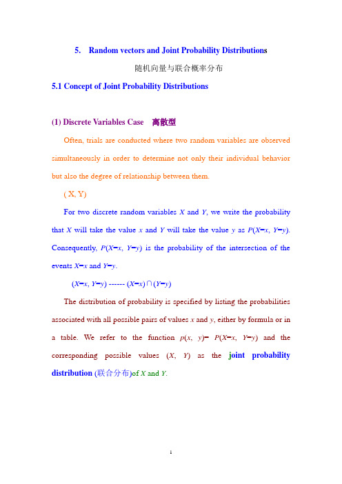
5. Random vectors and Joint Probability Distribution s随机向量与联合概率分布5.1 Concept of Joint Probability Distributions(1) Discrete Variables Case 离散型Often, trials are conducted where two random variables are observed simultaneously in order to determine not only their individual behavior but also the degree of relationship between them.( X, Y)For two discrete random variables X and Y, we write the probability that X will take the value x and Y will take the value y as P(X=x, Y=y). Consequently, P(X=x, Y=y) is the probability of the intersection of the events X=x and Y=y.(X=x, Y=y) ------ (X=x)∩(Y=y)The distribution of probability is specified by listing the probabilities associated with all possible pairs of values x and y, either by formula or in a table. We refer to the function p(x, y)=P(X=x, Y=y) and the corresponding possible values (X, Y) as the j oint probability distribution (联合分布)of X and Y.They satisfy(,)0, (,)1xyp x y p x y ≥=∑∑,where the sum is over all possible values of the variable.Example 5.1.1 Calculating probabilities from a discrete joint probability distributionLet X and Y have the joint probability distribution.(a) Find (1)P X Y +>;(b) Find the probability distribution ()()X p x P X x == of the individualrandom variable X . Solution(a) The event 1X Y +>is composed of the pairs of values (l,1), (2,0), and (2,l). Adding their corresponding probabilities(1)(1,1)(2,0)(2,1)0.20.100.3.P X Y p p p +>=++=++=(b) Since the event X =0 is composed of the two pairs of values (0,0) and (0,1), we add their corresponding probabilities to obtain(0)(0,0)(0,1)0.10.20.3P X p p ==+=+=.Continuing, we obtain (1)(1,0)(1,1)0.40.20.6P X p p ==+=+= and(2)(2,0)(2,1)0.100.1P X p p ==+=+=.In summary, (0)0.3X p =, (1)0.6X p = and (2)0.1X p =is the probabilitydistribution of X . Note that the probability distribution ()X p x of appears in the lower margin of this enlarged table. The probability distribution ()Y p y of Y appears in the right-hand margin of the table. Consequently, the individual distributions are called marginal probability distributions .（边缘分布）From the example, we see that for each fixed value of x , the marginalprobability distribution is obtained as()()(,)X yP X x p x p x y ===∑,where the sum is over all possible values of the second variable. Continuing, we obtain()()(,)Y xP Y y p y p x y ===∑.Example 3.5.3Suppose the number X of patent applications （专利申请）submitted by a company during a 1-year period is a random variable having thePoisson distribution with mean λ, (()!n e P X n n λλ-==)and the variousapplications independently have probability (0,1)p ∈ of eventually being approved.Determine the distribution of the number of patent applications during the 1-year period that are eventually approved.先求联合分布密度，再求边缘分布Solution Let Y be the number of patent application being eventually approved during 1-year period. Then the event {}Y k = is the union of mutually exclusive events {,}X n Y k == ()n k ≥.If X n =, then the random variable S has the binomial distribution with parameter n and p :(|)(1)k k n k n P Y k X n C p p -===-. (0)n k ≥≥ Thus(,)()(|)P X n Y k P X n P Y k X n ====== (1)!nk kn k n e C p p n λλ--=⋅⋅-when k>n, P(X=n, Y=k)=0,Hence the distribution of Y is()(,)(,)n n kP Y k P X n Y k P X n Y k ∞∞=========∑∑(1)!nk kn k n n ke C p p n λλ∞--==⋅⋅-∑!(1)!!()!nk n k n k n e p p n k n k λλ∞--==⋅⋅--∑(1)!()!kn kkn k n ke p p k n k λλλ-∞--==⋅⋅--∑()(1)(1)()()!!!mk k p m p p p e e ek m k λλλλλλ∞---=-==∑ ()!k pp e k λλ-= Thus, Y has the Poisson distribution of mean p λ. exercise从1，2，3，4，5五个数中不放回随机的接连地取3个，然后按大小排成123X X X <<，试求13(,)X X 的联合分布，x1,x3 独立吗？Homework Chap 5 1,(2) Continuous Variables Case 连续型随机向量There are many situations in which we describe an outcome by giving the values of several continuous random variables. For instance, we may measure the weight and the hardness of a rock, the pressure and the temperature of a gas. Suppose that X and Y are two continuous random variables. A function (,)f x y is called the joint probability density of these random variables, if the probability that , a X b c Y d ≤≤≤≤ is given by the multiple integral(, )(,)b da cP a X b c Y d f x y dxdy ≤≤≤≤=⎰⎰Thus, a function (,)f x y can serve as a joint probability density if all of the following hold:for all values of x and y , f is integrable on R 2 andTo extend the concept of a cumulative distribution function to the two variables case, we can define F (x , y )(, )(, )F x y P X x Y y =≤≤,and we refer to the corresponding function F as the joint cumulative distribution function of the two random variables.Example 5.1.2If the joint probability density of two random variables is given by236 for 0,0(,)0 elsewherex y e x y f x y --⎧>>=⎨⎩ Find the joint distribution function, and use it to find the probability(2,4)P X Y ≤≤.Solution By definition,23006 for 0, 0(,)(,)0 elsewhere y x yu vxe du e dv x y F x yf u v dudv ---∞-∞⎧>>⎪==⎨⎪⎩⎰⎰⎰⎰Thus,23(1)(1) for >0, >0(,)0 elsewhere x y e e x y F x y --⎧--=⎨⎩.Hence,412(2, 4)(2, 4)(1)(1)0.9817P X Y F e e --≤≤==--=.ExampleIf the joint probability density of two random variables is given by2,1,01(,)0,kxy x y x f x y ⎧≤≤≤≤=⎨⎩其他(a)find the k; (b)find the probability2((,)),{(,)|,01}P X Y D D x y x y x x ∈=≤≤≤≤solutionsince(,)1f x y dxdy ∞∞-∞-∞=⎰⎰24111001(,)()226x x kf x y dxdy dx kxydy k x dx ∞∞-∞-∞==-=⎰⎰⎰⎰⎰ hence k=6.21124001((,))663()4xx DP X Y D xydxdy dx xydy x x x dx ∈===-=⎰⎰⎰⎰⎰joint marginal densities 边缘密度Given the joint probability density of two random variables, the probability density of the X or Y can be obtained by integrating out another variable,The functions f X and f Y respectively are called the marginal density （边缘密度）of X and Y .,ExampleThe joint probability density of two random variables is given by26,1,01(,)0,xy x y x f x y ⎧≤≤≤≤=⎨⎩其他find the marginal density from the joint density when [0,1]x ∈，215()(,)633X xf x f x v dv xydy x x +∞-∞====-⎰⎰[0,1]x ∉，()0X f x =，hence 533,01()0,X x x x f x elsewhere ⎧-≤≤=⎨⎩23,01()0,Y y y f x elsewhere ⎧≤≤=⎨⎩exercises求服从B 上均匀分布的随机向量（X,Y ）的分布密度及分布函数。

概率与概率分布

第5章概率与概率分布一、思考题5.1、频率与概率有什么关系？5.2、独立性与互斥性有什么关系？5.3、根据自己的经验体会举几个服从泊松分布的随机变量的实例。

5.4、根据自己的经验体会举几个服从正态分布的随机变量的实例。

二、练习题5.1、写出下列随机试验的样本空间：（1）记录某班一次统计学测试的平均分数。

（2）某人在公路上骑自行车，观察该骑车人在遇到第一个红灯停下来以前遇到的绿灯次数。

（3）生产产品，直到有10件正品为止，记录生产产品的总件数。

5.2、某市有50%的住户订阅日报，有65%的住户订阅晚报，有85%的住户至少订两种报纸中的一种，求同时订这两种报纸的住户的百分比。

5.3、设A 与B 是两个随机事件，已知A 与B 至少有个发生的概率是31，A 发生且B 不发生的概率是91，求B 发现的概率。

5.4、设A 与B 是两个随机事件，已知P(A)=P(B)=31，P(A ｜B)= 61，求P(A ｜B ) 5.5、有甲、乙两批种子，发芽率分别是0.8和0.7。

在两批种子中各随机取一粒，试求：（1）两粒都发芽的概率。

（2）至少有一粒发芽的概率。

（3）恰有一粒发芽的概率。

5.6、某厂产品的合格率为96%，合格品中一级品率为75%，从产品中任取一件为一级品的概率是多少？5.7、某种品牌的电视机用到5000小时未坏的概率为43，用到10000小时未坏的概率为21。

现在有一台这种品牌的电视机已经用了5000小时未坏，它能用到10000小时的概率是多少？5.8、某厂职工中，小学文化程度的有10%，初中文化程度的有50%，高中及高中以上文化程度的有40%，25岁以下青年在小学、初中、高中及高中以上文化程度各组中的比例分别为20%，50%，70%。

从该厂随机抽取一名职工，发现年龄不到25岁，他具有小学、初中、高中及高中以上文化程度的概率各为多少？5.9、某厂有A ，B ，C ，D 四个车间生产同种产品，日产量分别占全厂产量的30%，27%，25%，18%。

概率统计c 5_2

11
Covariance
That is, since X – X and Y – Y are the deviations of the two variables from their respective mean values, the covariance is the expected product of deviations. Note that Cov(X, X) = E[(X – X)2] = V(X) V(X + Y) = V(X) + V(Y) + 2Cov(X,Y) The rationale for the definition is as follows.
13
Covariance
For a strong negative relationship, the signs of (x – X) and (y – Y) will tend to be opposite, yielding a negative product. Thus for a strong negative relationship, Cov(X, Y) should be quite negative. If X and Y are not strongly related, positive and negative products will tend to cancel one another, yielding a covariance near 0.
Where
X EX Y EY X and Y are V (X ) V (Y )

standardized rv of X and Y, respectively.
19
Example 17

概率论与数理统计第五章2

tα (n)
分布的上分位数或上侧临界值，的数tα(n)为t分布的上α分位数或上侧临界值，其几何意义见图5-7. 其几何意义见图
标准正态分布的分位数
在实际问题中，在实际问题中， α常取0.1、0.05、0.01. 常用到下面几个临界值：常用到下面几个临界值：
u0.05 =1.645，， u0.05/2=1.96，，
u0.01 =2.326 u0.01/2=2.575
数理统计中常用的分布除正态分布外，数理统计中常用的分布除正态分布外，还有三个非常有用的连续型分布，三个非常有用的连续型分布，即
定理5.1 定理5.1
设(X1，X2，…，Xn)为来自正态总体 X～N( ，σ 2)的样本，则的样本，～ (1) 样本均值 X与样本方差S 2相互独立；相互独立； n (2)
(n 1)S
2
σ
2
=
∑(X X)
i =1 i
2
σ
2
~ χ (n 1)
2
(5.8)
与以下补充性质的结论比较：与以下补充性质的结论比较：性质设(X1，X2，…，Xn)为取自正态总体
上侧临界值. 如图. 上侧临界值如图
概率分布的分位数(分位点) 概率分布的分位数(分位点) 定义对总体X和给定的α (0<α<1)，若存在xα， α 分布的上侧分位数或上侧α 使P{X≥xα} =α，则称xα为X分布的上侧α分位数或 α y α o xα x
P{X≥xα} =α α
∫ xα
其中Sn
(5.10)
=
2 (n1 1)S1
2 2 S1、S2 分别为两总体的样本方差分别为两总体的样本方差.
n1 + n2 2

概率统计：矩母函数

et (12
)(12
2 2
)t2
/
2
因而 X
Y
~
N (1
2 ,12
2 2
).
M X (t) E(etX )， M (n) (0) EX n， M X (t) etM X (t)，
X1, , Xn 独立 M X1 Xn (t) M X1 (t) M Xn (t)，
X 和Y 有相同分布 M X (t) MY (t).
定义 5.1 设 X 为随机变量,I 是一个包含0的(有限或无限的)
开区间,对任意t I ,期望EetX 存在,则称函数
M X (t) E(etX )
etxdF (x), t I
为 X 的矩母函数,常把M X (t)简记为M (t).因此
(离散型)
M X (t)
etxi P( X
i
xi ) ,
10
矩母函数(10)
例 5.4 设 X ~ N (, 2),求 X 的矩母函数.
解设Y ( X ) / ,则Y ~ N (0,1),MY (t) et2 / 2.因为
X Y ,故
M X (t) et MY ( t) et 2t2 / 2 .
11
作业
• 习题三: 34,35,36
12
命题 6.2
设 X ,Y 独立, X
~ N (1,12 ),
Y
~
N
(2,
2 2
)
,则
X
Y
~
N (1
2
,
2 1
2 2
)
证 M X (t) et112t2 / 2， MY (t) et2 22t2 / 2 ,故
M

1、下载文档前请自行甄别文档内容的完整性，平台不提供额外的编辑、内容补充、找答案等附加服务。
2、"仅部分预览"的文档,不可在线预览部分如存在完整性等问题,可反馈申请退款(可完整预览的文档不适用该条件!)。
3、如文档侵犯您的权益，请联系客服反馈,我们会尽快为您处理(人工客服工作时间：9:00-18:30)。

习题与解答5.2
1. 以下是某工厂通过抽样调查得到的10名工人一周内生产的产品数 149 156 160 138 149 153 153 169 156 156 试由这批数据构造经验分布函数并作图. 解此样本容量为10,经排序可得有序样本:
(1)(2)(3)(4)(5)(6)(7)(8)(9)(10)138,149,153,156,160,169x x x x x x x x x x ==========
其经验分布函数及其图形分别如下
()01380.11490.31530.51560.81600.91691n x F <⎧⎪≤<⎪
⎪≤<⎪=≤<⎨⎪≤<⎪
≤<⎪⎪
≥⎩，x ，
， 138x ，， 149x ，， 153x ，， 156x ，， 160x ，， x 169.
2. 下表是经过整理后得到的分组样本:
试写出此分组样本的经验分布函数. 解样本的经验分布函数为
()037.50.1547.50.3557.50.7567.50.977.51n x x F <⎧⎪≤<⎪
⎪≤<=⎨≤<⎪
⎪≤<⎪
≥⎩，，
， 37.5x ，， 47.5x ，
， 57.5x ，
， 67.5x ，， x 77.5.
3.假若某地区30名2000年某专业毕业生实习满后的月薪数据如下: 909 1086 1120 999 1320 1091 1071 1081 1130 1336 967 1572 825 914 992 1232 950 775 1203 1025 1096 808 1224 1044 871 1164 971 950 866 738 (1)构造该批数据的频率分布表(分6组); (2)画出直方图.
解此处数据最大观测值为1572,最小观测值为738,故组距近似为
1572736
140,6
d -=
= 确定每组区间端点为 ,此处可取 ,于是分组区间为
(](](](](](]735.875875101510151155115512951295143514351575
.，，，，，，，，，，其频数频率分布表如下:
其直方图如图5.2.
4.某公司对其250名职工上班所需时间进行了调查,下面是其不完整的频率分布表:
(1)试将频率分布表补充完整;
(2)该公司上班所需时间在半小时以内有多少人?
解(1)由于频率和为1,故空缺的频率为1-0.1-0.24-0.18-0.14=0.34. (2)该公司上班所需的时间在半小时以内的人所占频率为0.1+0.24+0.34=0.68,该公司有职工250人,故该公司上班所需时间在半
⨯=人.
小时以内的人有2500.68170
5. 40种刊物的月发行量如下(单位:百册):
(1)建立该批数据的频数分布表,取组距为1700百册;
5954 5022 14667 6582 6870 1840 2662 4508
1208 3852 618 3008 1268 1978 7963 2048
3077 993 353 14263 1714 11127 6926 2047 714 5923 6006 14267 1697 13876 4001 2280 1223 12579 13588 7315 4538 13304 1615 8612 (2)画出直方图.
解此处数据最大观测值为14667,最小观测值为353,由于组距为1700,故组数为14667353
8.421700
K -≥
=，
所以分9组.接下来确定每组区间端点,要求
03539170014667a
a <+⨯>，
此处可取0300a =，于是可列出其频数频率分布表.
其直方图为
6.对下列数据构造茎叶图
452 425 447 377 341 369 412 399
400 382 366 425 399 398 423 384
418 392 372 418 374 385 439 408
409 428 430 413 405 381 403 469
381 443 441 433 399 379 386 387
解取百位数与十位数组成茎,个位数为叶,这组数据的茎叶图如下:
34 1
35
36 6 9
37 2 4 7 9
38 1 1 2 4 5 6 7
39 2 8 9 9 9
40 0 3 5 8 9
41 2 3 8 8
42 3 5 5 8
43 0 3 9
44 1 3 7
45 2
46 9
7. 根据调查,某集团公司的中层管理人员的年薪数据如下(单位:千元):
40.6 39.6 37.8 36.2 38.8
38.6 39.6 40.0 34.7 41.7 38.9 37.9 37.0 35.1 36.7 37.1 37.7 39.2 36.9 39.3 试画出茎叶图.
解取整数部分为茎,小数部分为叶,这组数据的茎叶图如下: 34 7 35 1 36 2 7 9 37 0 1 7 8 9 38 3 6 8 9 39 2 6 6 40 0 6 41 7
8. 设总体X 的分布函数为()F x ,经验分布函数为()n F x ,试证
()()()()()1
1.n n E x F x Var x F x F x n
F F ⎡⎤⎡⎤==
-⎡⎤⎣⎦⎣⎦⎣⎦，证设1,...,n x x 是取自总体分布函数为()F x 的样本,则经验分布函数为
()()()110/12,..., 1.1.
k n
n x x x k n x x x k n x F +⎧<⎪⎪
=≤<=-⎨⎪>=⎪⎩（）（k ），当，
当，，，当x 若令{}12,...,i x x i i n y I ≤==，，
,则1,...,n y y 是独立同分布的随机变量,且 ()()()()()21111()E y P x x F x E y P x x F x =≤==≤=，，于是()()()()2
()[[1].]i Var F x F x F x F
x y =-=-
又()n x F 可写为()n x F =1
1n
i i n y =∑,故有
()()
()()()()1
111
,()1.n n E x E
F x Var x Var F x F x n
n y y F F ⎡⎤⎡⎤====-⎡⎤⎣⎦⎣⎦⎣⎦。