计量经济学第4章习题作业
【VIP专享】计量经济学第四章练习题及参考解答

(2) 3.060 1.657ln() 1.057ln()
(0.337) (0.092) (0.215)0.992 0.991 F 1275.093
GDP CPI R =-+-===进口居民消费价格指数的回归系数的符号不能进行合理的经济意义解释可能数据中有多重共线性。
计算相关系数:
22ln Y 4.09071.2186ln () t= (-10.6458) (34.6222)
0.9828 0.9820 1198.698
GDP R R F =-+===ln Y 5.4424 2.6637ln (PI)C =-+
从修正的可决系数和F统计量可以看出,全部变量对数线性多元回归整体对样本拟合很好,著。
可是其中的lnX3、lnX4、lnX6对lnY影响不显著,而且lnX2、lnX5
可以看出lnx1与lnx2、lnx3、lnx4、lnx5、lnx6之间高度相关,许多相关系数高于作为解释变量,很可能会出现严重多重共线性问题。
在本章开始的“引子”提出的“农业的发展反而会减少财政收入吗?
表4.13 1978-2007
财政收入(亿元)CS农业增加值(亿元)NZ工业增加值(亿元)GZ建筑业增加值
1132.31027.51607
1146.41270.21769.7
1159.91371.61996.5
1175.81559.52048.4
(1)根据样本数据得到各解释变量的样本相关系数矩阵如下:样本相关系数矩阵
解释变量之间相关系数较高,特别是农业增加值、工业增加值、建筑业增加值、最终消费之间,相关系数都在这显然与第三章对模型的无多重共线性假定不符合。
计量经济学第四章习题(龚志民)fixed
第四章 多元线性回归模型的估计与假设检验问题4.1什么是偏回归系数? 答:在总体回归函数12233k k Y X X X u ββββ=+++++中,系数2,,k ββ被称为斜率系数或偏回归系数。
(多元样本回归函数的系数亦称偏回归系数)4.2什么是完全多重共线性?什么是高度共线性(近似完全共线性)?答:对于解释变量123,,...k X X X X ,如果存在不全为0的数123,,...k λλλλ,使得112233...0k k X X X X λλλλ++++=则称解释变量之间存在着完全的多重共线性。
如果解释变量123,,...k X X X X 之间存在较大的相关性,但又不是完全共线性,则称解释变量之间存在不完全多重共线性。
4.3 多元回归方程中偏回归系数与一元回归方程中回归系数的含义有何差别? 答:相同点:两者都表示当X 每变化一单位时,Y 的均值的变化。
不同点:偏回归系数是表示当其他解释变量不变时,这一解释变量对被解释变量的影响。
而回归系数则不存在其他解释变量,也就不需要对其他变量进行限制。
4.4 几个变量“联合显著”的含义是什么?答:联合显著的含义是,几个变量作为一个集体是显著的。
即在它们的系数同时为0的假设下,统计量超过临界值。
直观的意义是,它们的系数同时为零的可能性很小。
习题4.5下表中的数据23,,Y X X 分别表示每周销售量,每周的广告投入和每周顾客的平均收入(见DATA4-5)(1)估计回归方程12233()E Y X X βββ=++。
(2)计算拟合优度。
(3)计算校正拟合优度。
(4)计算2β的置信区间(置信水平为95%)。
(5)检验假设03H :0β=(备择假设13H :0β≠,显著性水平为5%) (6)检验假设03H :0β=(备择假设13H :0β>,显著性水平为5%)(7)检验建设023H :0ββ==(显著性水平为5%)。
答:(1)由eviews6.0输出结果:可知1ˆ109.4β=,23ˆˆ2.835714, 5.125714ββ== 回归方程为:23()109.4 2.835714 5.125714E Y X X =++(2)由输出结果可以得到拟合优度为0.910086。
《计量经济学》习题(第四章)

《计量经济学》习题(第四章)第四章习题⼀、单选题1、如果回归模型违背了同⽅差假定,最⼩⼆乘估计量____A .⽆偏的,⾮有效的 B.有偏的,⾮有效的C .⽆偏的,有效的 D.有偏的,有效的2、Goldfeld-Quandt ⽅法⽤于检验____A .异⽅差性 B.⾃相关性C .随机解释变量 D.多重共线性3、DW 检验⽅法⽤于检验____A .异⽅差性 B.⾃相关性C .随机解释变量 D.多重共线性4、在异⽅差性情况下,常⽤的估计⽅法是____A .⼀阶差分法 B.⼴义差分法C .⼯具变量法 D.加权最⼩⼆乘法5、在以下选项中,正确表达了序列⾃相关的是____j i u x Cov D j i x x Cov C ji u u Cov B ji u u Cov A j i j i j i j i ≠≠≠≠≠=≠≠,0),(.,0),(.,0),(.,0),(.6、如果回归模型违背了⽆⾃相关假定,最⼩⼆乘估计量____A .⽆偏的,⾮有效的 B.有偏的,⾮有效的C .⽆偏的,有效的 D.有偏的,有效的7、在⾃相关情况下,常⽤的估计⽅法____A .普通最⼩⼆乘法 B.⼴义差分法C .⼯具变量法 D.加权最⼩⼆乘法8、White 检验⽅法主要⽤于检验____A .异⽅差性 B.⾃相关性C .随机解释变量 D.多重共线性9、Glejser 检验⽅法主要⽤于检验____A .异⽅差性 B.⾃相关性C .随机解释变量 D.多重共线性10、简单相关系数矩阵⽅法主要⽤于检验____A .异⽅差性 B.⾃相关性C .随机解释变量 D.多重共线性2222)(.)(.)(.)(.σσσσ==≠≠i i i i x Var D u Var C x Var B u Var A12、所谓不完全多重共线性是指存在不全为零的数k λλλ,,,21 ,有____1112211221221122.0.0..k k k k k x x x k k k k A x x x v B x x x C x x x v e D x x x v e v λλλλλλλλλλλλ++++=+++=∑?++++=++++=式中是随机误差项13、设21,x x 为解释变量,则完全多重共线性是____0.(021.0.021.22121121=+=++==+x x e x D v v x x C e x B x x A 为随机误差项)14、⼴义差分法是对____⽤最⼩⼆乘法估计其参数 11211211121121)()1(....-------+-+-=-++=++=++=t t t t t t t t t t t t t t t u u x x y y D u x y C u x y B u x y A ρρβρβρρρβρβρββββ15、在DW 检验中要求有假定条件,在下列条件中不正确的是____A .解释变量为⾮随机的 B.随机误差项为⼀阶⾃回归形式C .线性回归模型中不应含有滞后内⽣变量为解释变量D.线性回归模型为⼀元回归形式16、在下例引起序列⾃相关的原因中,不正确的是____A.经济变量具有惯性作⽤B.经济⾏为的滞后性C.设定偏误D.解释变量之间的共线性17、在DW 检验中,当d 统计量为2时,表明____A.存在完全的正⾃相关B.存在完全的负⾃相关C.不存在⾃相关D.不能判定18、在DW 检验中,当d 统计量为4时,表明____A.存在完全的正⾃相关B.存在完全的负⾃相关C.不存在⾃相关D.不能判定19、在DW 检验中,当d 统计量为0时,表明____A.存在完全的正⾃相关C.不存在⾃相关D.不能判定20、在DW 检验中,存在不能判定的区域是____A. 0﹤d ﹤l d ,4-l d ﹤d ﹤4B. u d ﹤d ﹤4-u dC. l d ﹤d ﹤u d ,4-u d ﹤d ﹤4-l dD. 上述都不对21、在修正序列⾃相关的⽅法中,能修正⾼阶⾃相关的⽅法是____A. 利⽤DW 统计量值求出ρB. Cochrane-Orcutt 法C. Durbin 两步法D. 移动平均法22、在下列多重共线性产⽣的原因中,不正确的是____A.经济本变量⼤多存在共同变化趋势B.模型中⼤量采⽤滞后变量C.由于认识上的局限使得选择变量不当D.解释变量与随机误差项相关23、在DW 检验中,存在正⾃相关的区域是____A. 4-l d ﹤d ﹤4B. 0﹤d ﹤l dC. u d ﹤d ﹤4-u dD. l d ﹤d ﹤u d ,4-u d ﹤d ﹤4-l d24、逐步回归法既检验⼜修正了____A .异⽅差性 B.⾃相关性 C .随机解释变量 D.多重共线性25、设)()(,2221i i i i i ix f u Var u x y σσββ==++=,则对原模型变换的正确形式为____ )()()()(.)()()()(.)()()()(..212222122121i i i i i i i i i i i i i i i i i i i i i i i i x f u x f x x f x f y D x f u x f x x f x f y C x f u x f x x f x f y B u x y A ++=++=++=++=ββββββββ 26、在修正序列⾃相关的⽅法中,不正确的是____A.⼴义差分法B.普通最⼩⼆乘法C.⼀阶差分法D. Durbin 两步法27、在检验异⽅差的⽅法中,不正确的是____A. Goldfeld-Quandt ⽅法B. spearman 检验法C. White 检验法28、在DW 检验中,存在零⾃相关的区域是____A. 4-l d ﹤d ﹤4B. 0﹤d ﹤l dC. u d ﹤d ﹤4-u dD. l d ﹤d ﹤u d ,4-u d ﹤d ﹤4-l d29.如果模型中的解释变量存在完全的多重共线性,参数的最⼩⼆乘估计量是()A .⽆偏的 B. 有偏的 C. 不确定 D. 确定的30. 已知模型的形式为u x y 21+β+β=,在⽤实际数据对模型的参数进⾏估计的时候,测得DW 统计量为0.6453,则⼴义差分变量是( )A. 1t t ,1t t x 6453.0x y 6453.0y ----B. 1t t 1t t x 6774.0x ,y 6774.0y ----C. 1t t 1t t x x ,y y ----D. 1t t 1t t x 05.0x ,y 05.0y ----31. 在具体运⽤加权最⼩⼆乘法时,如果变换的结果是x u x x x 1xy 21+β+β=,则Var(u)是下列形式中的哪⼀种?( )A. 2σxB. 2σ2x B. 2σx D. 2σLog(x)32. 在线性回归模型中,若解释变量1x 和2x 的观测值成⽐例,即有i 2i 1kx x =,其中k 为⾮零常数,则表明模型中存在( )A. 异⽅差B. 多重共线性C. 序列⾃相关D. 设定误差33. 已知DW 统计量的值接近于2,则样本回归模型残差的⼀阶⾃相关系数ρ近似等于( ) A. 0 B. –1 C. 1 D. 4⼆、多项选择1、能够检验多重共线性的⽅法有____A.简单相关系数法B. DW检验法C. 判定系数检验法D. ⽅差膨胀因⼦检验E.逐步回归法2、能够修正多重共线性的⽅法有____A.增加样本容量B.岭回归法C.剔除多余变量E.差分模型3、如果模型中存在异⽅差现象,则会引起如下后果____A. 参数估计值有偏B. 参数估计值的⽅差不能正确确定C. 变量的显著性检验失效D. 预测精度降低E. 参数估计值仍是⽆偏的4、能够检验异⽅差的⽅法是____A. gleiser检验法B. White检验法C. 图形法D. spearman检验法E. DW检验法F. Goldfeld-Quandt检验法5、如果模型中存在序列⾃相关现象,则会引起如下后果____A. 参数估计值有偏B. 参数估计值的⽅差不能正确确定C. 变量的显著性检验失效D. 预测精度降低E. 参数估计值仍是⽆偏的6、检验序列⾃相关的⽅法是____A. gleiser检验法B. White检验法C. 图形法D. DW检验法E. Goldfeld-Quandt检验法7、能够修正序列⾃相关的⽅法有____A. 加权最⼩⼆乘法B. Durbin两步法C. ⼴义最⼩⼆乘法D. ⼀阶差分法E. ⼴义差分法8、Goldfeld-Quandt检验法的应⽤条件是____A. 将观测值按解释变量的⼤⼩顺序排列B. 样本容量尽可能⼤C. 随机误差项服从正态分布D. 将排列在中间的约1/4的观测值删除掉9、在DW检验中,存在不能判定的区域是____A. 0﹤d﹤l dB. u d﹤d﹤4-u dC. l d﹤d﹤u dD. 4-u d﹤d﹤4-l dE. 4-l d﹤d﹤4。
(完整word版)计量经济学第四章习题详解

第四章习题4.1 没有进行t检验,并且调整的可决系数也没有写出来,也就是没有考虑自由度的影响,会使结果存在误差.4.3200224430.3120332。
7 330.6200334195。
6135822.8 334。
6200446435.8159878.3 l347.7200554273.7183084.8 353.9200663376.9211923。
5 359。
2200773284。
6249529。
9 376.5200879526.5314045.4 398.7200968618。
4340902。
8 395。
9201094699.3401512.8 408。
92011113161.4472881.6 431.0一研究的目的和要求我们知道,商品进口额与很多因素有关,了解其变化对进出口产品有很大帮助。
为了探究和预测商品进口额的变化,需要定量地分析影响商品进口额变化的主要因素。
二、模型的设定及其估计经分析,商品进口额可能与国内生产总值、居民消费价格指数有关。
为此,考虑国内生产总值GDP、居民消费价格指数CPI为主要因素。
各影响变量与商品进口额呈正相关。
为此,设定如下形式的计量经济模型:=+ln+lnCP式中,亿元);lnGDP为国内生产总值(亿元);lnCPI为居民消费价格指数(以1985年为100)。
各解释变量前的回归系数预期都大于零。
为估计模型,根据上表的数据,利用EViews软件,生成Y、lnGDP、lnCPI等数据,采用OLS方法估计模型参数,得到的回归结果如下图所示:模型方程为:lnY=-3。
111486+1。
338533lnGDP-0.421791lnCPI(0。
463010)(0。
088610)(0。
233295)t= (—6。
720126) (15。
10582)(—1。
807975)=0.988051 =0.987055 F=992。
2582该模型=0.988051,=0。
987055,可决系数很高,F检验值为992.2582,明显显著。
《计量经济学》习题(第四章)
第四章 习 题一、单选题1、如果回归模型违背了同方差假定,最小二乘估计量____A .无偏的,非有效的 B.有偏的,非有效的C .无偏的,有效的 D.有偏的,有效的2、Goldfeld-Quandt 方法用于检验____A .异方差性 B.自相关性C .随机解释变量 D.多重共线性3、DW 检验方法用于检验____A .异方差性 B.自相关性C .随机解释变量 D.多重共线性4、在异方差性情况下,常用的估计方法是____A .一阶差分法 B.广义差分法C .工具变量法 D.加权最小二乘法5、在以下选项中,正确表达了序列自相关的是____j i u x Cov D j i x x Cov C ji u u Cov B ji u u Cov A j i j i j i j i ≠≠≠≠≠=≠≠,0),(.,0),(.,0),(.,0),(.6、如果回归模型违背了无自相关假定,最小二乘估计量____A .无偏的,非有效的 B.有偏的,非有效的C .无偏的,有效的 D.有偏的,有效的7、在自相关情况下,常用的估计方法____A .普通最小二乘法 B.广义差分法C .工具变量法 D.加权最小二乘法8、White 检验方法主要用于检验____A .异方差性 B.自相关性C .随机解释变量 D.多重共线性9、Glejser 检验方法主要用于检验____A .异方差性 B.自相关性C .随机解释变量 D.多重共线性10、简单相关系数矩阵方法主要用于检验____A .异方差性 B.自相关性C .随机解释变量 D.多重共线性11、所谓异方差是指____2222)(.)(.)(.)(.σσσσ==≠≠i i i i x Var D u Var C x Var B u Var A12、所谓不完全多重共线性是指存在不全为零的数k λλλ,,,21 ,有____1112211221221122.0.0..k k k k k x x x k k k k A x x x v B x x x C x x x v e D x x x v e v λλλλλλλλλλλλ++++=+++=∑⎰++++=++++=式中是随机误差项13、设21,x x 为解释变量,则完全多重共线性是____0.(021.0.021.22121121=+=++==+x x e x D v v x x C e x B x x A 为随机误差项) 14、广义差分法是对____用最小二乘法估计其参数11211211121121)()1(....-------+-+-=-++=++=++=t t t t t t t t t t t t tt t u u x x y y D u x y C u x y B u x y A ρρβρβρρρβρβρββββ15、在DW 检验中要求有假定条件,在下列条件中不正确的是____A .解释变量为非随机的 B.随机误差项为一阶自回归形式C .线性回归模型中不应含有滞后内生变量为解释变量D.线性回归模型为一元回归形式16、在下例引起序列自相关的原因中,不正确的是____A.经济变量具有惯性作用B.经济行为的滞后性C.设定偏误D.解释变量之间的共线性17、在DW 检验中,当d 统计量为2时,表明____A.存在完全的正自相关B.存在完全的负自相关C.不存在自相关D.不能判定18、在DW 检验中,当d 统计量为4时,表明____A.存在完全的正自相关B.存在完全的负自相关C.不存在自相关D.不能判定19、在DW 检验中,当d 统计量为0时,表明____A.存在完全的正自相关B.存在完全的负自相关C.不存在自相关D.不能判定20、在DW 检验中,存在不能判定的区域是____A. 0﹤d ﹤l d ,4-l d ﹤d ﹤4B. u d ﹤d ﹤4-u dC. l d ﹤d ﹤u d ,4-u d ﹤d ﹤4-l dD. 上述都不对21、在修正序列自相关的方法中,能修正高阶自相关的方法是____A. 利用DW 统计量值求出ρˆ B. Cochrane-Orcutt 法 C. Durbin 两步法 D. 移动平均法22、在下列多重共线性产生的原因中,不正确的是____A.经济本变量大多存在共同变化趋势B.模型中大量采用滞后变量C.由于认识上的局限使得选择变量不当D.解释变量与随机误差项相关23、在DW 检验中,存在正自相关的区域是____A. 4-l d ﹤d ﹤4B. 0﹤d ﹤l dC. u d ﹤d ﹤4-u dD. l d ﹤d ﹤u d ,4-u d ﹤d ﹤4-l d24、逐步回归法既检验又修正了____A .异方差性 B.自相关性 C .随机解释变量 D.多重共线性25、设)()(,2221i i i i i i x f u Var u x y σσββ==++=,则对原模型变换的正确形式为____ )()()()(.)()()()(.)()()()(..212222122121i i i i i i i i i i i i i i i i i i i i i i i i x f u x f x x f x f y D x f u x f x x f x f y C x f u x f x x f x f y B u x y A ++=++=++=++=ββββββββ26、在修正序列自相关的方法中,不正确的是____A.广义差分法B.普通最小二乘法C.一阶差分法D. Durbin 两步法27、在检验异方差的方法中,不正确的是____A. Goldfeld-Quandt 方法B. spearman 检验法C. White 检验法D. DW 检验法28、在DW 检验中,存在零自相关的区域是____A. 4-l d ﹤d ﹤4B. 0﹤d ﹤l dC. u d ﹤d ﹤4-u dD. l d ﹤d ﹤u d ,4-u d ﹤d ﹤4-l d29.如果模型中的解释变量存在完全的多重共线性,参数的最小二乘估计量是( )A .无偏的 B. 有偏的 C. 不确定 D. 确定的30. 已知模型的形式为u x y 21+β+β=,在用实际数据对模型的参数进行估计的时候,测得DW 统计量为0.6453,则广义差分变量是( )A. 1t t ,1t t x 6453.0x y 6453.0y ----B. 1t t 1t t x 6774.0x ,y 6774.0y ----C. 1t t 1t t x x ,y y ----D. 1t t 1t t x 05.0x ,y 05.0y ----31. 在具体运用加权最小二乘法时,如果变换的结果是x u x x x 1xy 21+β+β=,则Var(u)是下列形式中的哪一种?( )A. 2σxB. 2σ2x B. 2σx D. 2σLog(x)32. 在线性回归模型中,若解释变量1x 和2x 的观测值成比例,即有i 2i 1kx x =,其中k 为非零常数,则表明模型中存在( )A. 异方差B. 多重共线性C. 序列自相关D. 设定误差33. 已知DW 统计量的值接近于2,则样本回归模型残差的一阶自相关系数ρˆ近似等于( ) A. 0 B. –1 C. 1 D. 4二、多项选择1、能够检验多重共线性的方法有____A.简单相关系数法B. DW 检验法C. 判定系数检验法D. 方差膨胀因子检验E.逐步回归法3、能够修正多重共线性的方法有____A.增加样本容量B.岭回归法C.剔除多余变量D.逐步回归法E.差分模型3、如果模型中存在异方差现象,则会引起如下后果____A. 参数估计值有偏B. 参数估计值的方差不能正确确定C. 变量的显著性检验失效D. 预测精度降低E. 参数估计值仍是无偏的4、能够检验异方差的方法是____A. gleiser检验法B. White检验法C. 图形法D. spearman检验法E. DW检验法F. Goldfeld-Quandt检验法5、如果模型中存在序列自相关现象,则会引起如下后果____A. 参数估计值有偏B. 参数估计值的方差不能正确确定C. 变量的显著性检验失效D. 预测精度降低E. 参数估计值仍是无偏的6、检验序列自相关的方法是____A. gleiser检验法B. White检验法C. 图形法D. DW检验法E. Goldfeld-Quandt检验法7、能够修正序列自相关的方法有____A. 加权最小二乘法B. Durbin两步法C.广义最小二乘法D. 一阶差分法E.广义差分法8、Goldfeld-Quandt检验法的应用条件是____A. 将观测值按解释变量的大小顺序排列B. 样本容量尽可能大C. 随机误差项服从正态分布D. 将排列在中间的约1/4的观测值删除掉9、在DW检验中,存在不能判定的区域是____A. 0﹤d﹤l dB. u d﹤d﹤4-u dC. l d﹤d﹤u dD. 4-u d﹤d﹤4-l dE. 4-l d﹤d﹤4。
计量经济学课后答案第四、五章(内容参考)
计量经济学课后答案第四、五章(内容参考)第四章随机解释变量问题1. 随机解释变量的来源有哪些?答:随机解释变量的来源有:经济变量的不可控,使得解释变量观测值具有随机性;由于随机干扰项中包括了模型略去的解释变量,而略去的解释变量与模型中的解释变量往往是相关的;模型中含有被解释变量的滞后项,而被解释变量本身就是随机的。
2.随机解释变量有几种情形? 分情形说明随机解释变量对最小二乘估计的影响与后果?答:随机解释变量有三种情形,不同情形下最小二乘估计的影响和后果也不同。
(1)解释变量是随机的,但与随机干扰项不相关;这时采用OLS估计得到的参数估计量仍为无偏估计量;(2)解释变量与随机干扰项同期无关、不同期相关;这时OLS估计得到的参数估计量是有偏但一致的估计量;(3)解释变量与随机干扰项同期相关;这时OLS估计得到的参数估计量是有偏且非一致的估计量。
3. 选择作为工具变量的变量必须满足那些条件?答:选择作为工具变量的变量需满足以下三个条件:(1)与所替代的随机解释变量高度相关;(2)与随机干扰项不相关;(3)与模型中其他解释变量不相关,以避免出现多重共线性。
4.对模型Y t =β+β1X1t+β2X2t+β3Yt-1+μt假设Yt-1与μt相关。
为了消除该相关性,采用工具变量法:先求Y t关于X1t与 X2t回归,得到Yt,再做如下回归:Y t =β+β1X1t+β2X2t+β3Y t?1-+μt试问:这一方法能否消除原模型中Yt的相关性? 为什么?解答:能消除。
在基本假设下,X1t,X2t与μt应是不相关的,由此知,由X1t 与X2t估计出的Yt应与μt不相关。
5.对于一元回归模型Y t =β+β1Xt*+μt假设解释变量Xt *的实测值Xt与之有偏误:Xt= Xt*+et,其中et是具有零均值、无序列相关,且与Xt不相关的随机变量。
试问:(1) 能否将X t= X t*+e t代入原模型,使之变换成Y t=β0+β1X t+νt后进行估计? 其中,νt为变换后模型的随机干扰项。
伍德里奇---计量经济学第4章部分计算机习题详解(MATLAB)
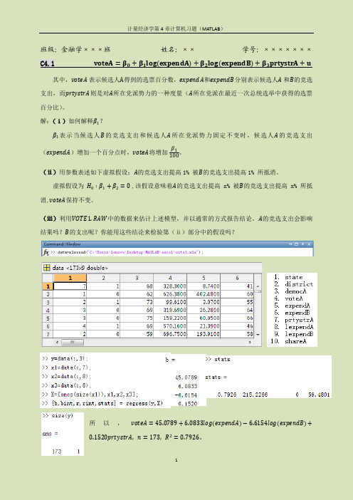
班级:金融学×××班姓名:××学号:×××××××C4.1 voteA=β0+β1log expendA+β2log expendB+β3prtystrA+u 其中,voteA表示候选人A得到的选票百分数,expendA和expendB分别表示候选人A和B的竞选支出,而prtystrA则是对A所在党派势力的一种度量(A所在党派在最近一次总统选举中获得的选票百分比)。
解:(ⅰ)如何解释β1?β1表示当候选人B的竞选支出和候选人A所在党派势力固定不变时,候选人A的竞选支出(expendA)增加一个百分点时,voteA将增加β1 100。
(ⅱ)用参数表述如下虚拟假设:A的竞选支出提高1% 被B的竞选支出提高1% 所抵消。
虚拟假设为H0∶β1+β2=0 ,该假设意味着A的竞选支出提高x% 被B的竞选支出提高x% 所抵消,voteA保持不变。
(ⅲ)利用VOTE1.RAW中的数据来估计上述模型,并以通常的方式报告结论。
A的竞选支出会影响结果吗?B的支出呢?你能用这些结论来检验第(ⅱ)部分中的假设吗?所以,voteA=45.0789+6.0833log expendA−6.6154log expendB+0.1520prtystrA, n=173, R2=0.7926 .由截图可得:expendA 系数β1的 t 统计量为15.9187,在很小的显著水平上都是显著的,意味着当其他条件不变时,A 的竞选支出增加1%,voteA 将增加0.0608。
同理可得,expendB 系数β2的 t 统计量为-17.4632,在很小的显著水平上都是显著的,意味着当其他条件不变时,B 的竞选支出增加1%,voteA 将增加0.066。
由于A 的竞选支出的系数β1和B 的竞选支出的系数β2符号相反,绝对值差不多,所以近似有虚拟假设“ H 0∶β1+β2=0 ”成立,即第(ⅱ)部分中的假设成立。
计量经济学第4章课后答案

17CHAPTER 4SOLUTIONS TO PROBLEMS4.2 (i) and (iii) generally cause the t statistics not to have a t distribution under H 0.Homoskedasticity is one of the CLM assumptions. An important omitted variable violates Assumption MLR.3. The CLM assumptions contain no mention of the sample correlations among independent variables, except to rule out the case where the correlation is one.4.3 (i) While the standard error on hrsemp has not changed, the magnitude of the coefficient has increased by half. The t statistic on hrsemp has gone from about –1.47 to –2.21, so now the coefficient is statistically less than zero at the 5% level. (From Table G.2 the 5% critical value with 40 df is –1.684. The 1% critical value is –2.423, so the p -value is between .01 and .05.)(ii) If we add and subtract 2βlog(employ ) from the right-hand-side and collect terms, we havelog(scrap ) = 0β + 1βhrsemp + [2βlog(sales) – 2βlog(employ )] + [2βlog(employ ) + 3βlog(employ )] + u = 0β + 1βhrsemp + 2βlog(sales /employ ) + (2β + 3β)log(employ ) + u ,where the second equality follows from the fact that log(sales /employ ) = log(sales ) – log(employ ). Defining 3θ ≡ 2β + 3β gives the result.(iii) No. We are interested in the coefficient on log(employ ), which has a t statistic of .2, which is very small. Therefore, we conclude that the size of the firm, as measured by employees, does not matter, once we control for training and sales per employee (in a logarithmic functional form).(iv) The null hypothesis in the model from part (ii) is H 0:2β = –1. The t statistic is [–.951 – (–1)]/.37 = (1 – .951)/.37 ≈ .132; this is very small, and we fail to reject whether we specify a one- or two-sided alternative.4.4 (i) In columns (2) and (3), the coefficient on profmarg is actually negative, although its t statistic is only about –1. It appears that, once firm sales and market value have been controlled for, profit margin has no effect on CEO salary.(ii) We use column (3), which controls for the most factors affecting salary. The t statistic on log(mktval ) is about 2.05, which is just significant at the 5% level against a two-sided alternative.18(We can use the standard normal critical value, 1.96.) So log(mktval ) is statistically significant. Because the coefficient is an elasticity, a ceteris paribus 10% increase in market value is predicted to increase salary by 1%. This is not a huge effect, but it is not negligible, either.(iii) These variables are individually significant at low significance levels, with t ceoten ≈ 3.11 and t comten ≈ –2.79. Other factors fixed, another year as CEO with the company increases salary by about 1.71%. On the other hand, another year with the company, but not as CEO, lowers salary by about .92%. This second finding at first seems surprising, but could be related to the “superstar” effect: firms that hire CEOs from outside the company often go after a small pool of highly regarded candidates, and salaries of these people are bid up. More non-CEO years with a company makes it less likely the person was hired as an outside superstar.4.7 (i) .412 ± 1.96(.094), or about .228 to .596.(ii) No, because the value .4 is well inside the 95% CI.(iii) Yes, because 1 is well outside the 95% CI.4.8 (i) With df = 706 – 4 = 702, we use the standard normal critical value (df = ∞ in Table G.2), which is 1.96 for a two-tailed test at the 5% level. Now t educ = −11.13/5.88 ≈ −1.89, so |t educ | = 1.89 < 1.96, and we fail to reject H 0: educ β = 0 at the 5% level. Also, t age ≈ 1.52, so age is also statistically insignificant at the 5% level.(ii) We need to compute the R -squared form of the F statistic for joint significance. But F = [(.113 − .103)/(1 − .113)](702/2) ≈ 3.96. The 5% critical value in the F 2,702 distribution can be obtained from Table G.3b with denominator df = ∞: cv = 3.00. Therefore, educ and age are jointly significant at the 5% level (3.96 > 3.00). In fact, the p -value is about .019, and so educ and age are jointly significant at the 2% level.(iii) Not really. These variables are jointly significant, but including them only changes the coefficient on totwrk from –.151 to –.148.(iv) The standard t and F statistics that we used assume homoskedasticity, in addition to the other CLM assumptions. If there is heteroskedasticity in the equation, the tests are no longer valid.4.11 (i) Holding profmarg fixed, n rdintensΔ = .321 Δlog(sales ) = (.321/100)[100log()sales ⋅Δ] ≈ .00321(%Δsales ). Therefore, if %Δsales = 10, n rdintens Δ ≈ .032, or only about 3/100 of a percentage point. For such a large percentage increase in sales,this seems like a practically small effect.(ii) H 0:1β = 0 versus H 1:1β > 0, where 1β is the population slope on log(sales ). The t statistic is .321/.216 ≈ 1.486. The 5% critical value for a one-tailed test, with df = 32 – 3 = 29, is obtained from Table G.2 as 1.699; so we cannot reject H 0 at the 5% level. But the 10% criticalvalue is 1.311; since the t statistic is above this value, we reject H0 in favor of H1 at the 10% level.(iii) Not really. Its t statistic is only 1.087, which is well below even the 10% critical value for a one-tailed test.1920SOLUTIONS TO COMPUTER EXERCISESC4.1 (i) Holding other factors fixed,111log()(/100)[100log()](/100)(%),voteA expendA expendA expendA βββΔ=Δ=⋅Δ≈Δwhere we use the fact that 100log()expendA ⋅Δ ≈ %expendA Δ. So 1β/100 is the (ceteris paribus) percentage point change in voteA when expendA increases by one percent.(ii) The null hypothesis is H 0: 2β = –1β, which means a z% increase in expenditure by A and a z% increase in expenditure by B leaves voteA unchanged. We can equivalently write H 0: 1β + 2β = 0.(iii) The estimated equation (with standard errors in parentheses below estimates) isn voteA = 45.08 + 6.083 log(expendA ) – 6.615 log(expendB ) + .152 prtystrA(3.93) (0.382) (0.379) (.062) n = 173, R 2 = .793.The coefficient on log(expendA ) is very significant (t statistic ≈ 15.92), as is the coefficient on log(expendB ) (t statistic ≈ –17.45). The estimates imply that a 10% ceteris paribus increase in spending by candidate A increases the predicted share of the vote going to A by about .61percentage points. [Recall that, holding other factors fixed, n voteAΔ≈(6.083/100)%ΔexpendA ).] Similarly, a 10% ceteris paribus increase in spending by B reduces n voteAby about .66 percentage points. These effects certainly cannot be ignored.While the coefficients on log(expendA ) and log(expendB ) are of similar magnitudes (andopposite in sign, as we expect), we do not have the standard error of 1ˆβ + 2ˆβ, which is what we would need to test the hypothesis from part (ii).(iv) Write 1θ = 1β +2β, or 1β = 1θ– 2β. Plugging this into the original equation, and rearranging, givesn voteA = 0β + 1θlog(expendA ) + 2β[log(expendB ) – log(expendA )] +3βprtystrA + u ,When we estimate this equation we obtain 1θ≈ –.532 and se( 1θ)≈ .533. The t statistic for the hypothesis in part (ii) is –.532/.533 ≈ –1. Therefore, we fail to reject H 0: 2β = –1β.21C4.3 (i) The estimated model isn log()price = 11.67 + .000379 sqrft + .0289 bdrms (0.10) (.000043) (.0296)n = 88, R 2 = .588.Therefore, 1ˆθ= 150(.000379) + .0289 = .0858, which means that an additional 150 square foot bedroom increases the predicted price by about 8.6%.(ii) 2β= 1θ – 1501β, and solog(price ) = 0β+ 1βsqrft + (1θ – 1501β)bdrms + u= 0β+ 1β(sqrft – 150 bdrms ) + 1θbdrms + u .(iii) From part (ii), we run the regressionlog(price ) on (sqrft – 150 bdrms ), bdrms ,and obtain the standard error on bdrms . We already know that 1ˆθ= .0858; now we also getse(1ˆθ) = .0268. The 95% confidence interval reported by my software package is .0326 to .1390(or about 3.3% to 13.9%).C4.5 (i) If we drop rbisyr the estimated equation becomesn log()salary = 11.02 + .0677 years + .0158 gamesyr (0.27) (.0121) (.0016)+ .0014 bavg + .0359 hrunsyr (.0011) (.0072)n = 353, R 2= .625.Now hrunsyr is very statistically significant (t statistic ≈ 4.99), and its coefficient has increased by about two and one-half times.(ii) The equation with runsyr , fldperc , and sbasesyr added is22n log()salary = 10.41 + .0700 years + .0079 gamesyr(2.00) (.0120) (.0027)+ .00053 bavg + .0232 hrunsyr (.00110) (.0086)+ .0174 runsyr + .0010 fldperc – .0064 sbasesyr (.0051) (.0020) (.0052) n = 353, R 2 = .639.Of the three additional independent variables, only runsyr is statistically significant (t statistic = .0174/.0051 ≈ 3.41). The estimate implies that one more run per year, other factors fixed,increases predicted salary by about 1.74%, a substantial increase. The stolen bases variable even has the “wrong” sign with a t statistic of about –1.23, while fldperc has a t statistic of only .5. Most major league baseball players are pretty good fielders; in fact, the smallest fldperc is 800 (which means .800). With relatively little variation in fldperc , it is perhaps not surprising that its effect is hard to estimate.(iii) From their t statistics, bavg , fldperc , and sbasesyr are individually insignificant. The F statistic for their joint significance (with 3 and 345 df ) is about .69 with p -value ≈ .56. Therefore, these variables are jointly very insignificant.C4.7 (i) The minimum value is 0, the maximum is 99, and the average is about 56.16. (ii) When phsrank is added to (4.26), we get the following:n log() wage = 1.459 − .0093 jc + .0755 totcoll + .0049 exper + .00030 phsrank (0.024) (.0070) (.0026) (.0002) (.00024)n = 6,763, R 2 = .223So phsrank has a t statistic equal to only 1.25; it is not statistically significant. If we increase phsrank by 10, log(wage ) is predicted to increase by (.0003)10 = .003. This implies a .3% increase in wage , which seems a modest increase given a 10 percentage point increase in phsrank . (However, the sample standard deviation of phsrank is about 24.)(iii) Adding phsrank makes the t statistic on jc even smaller in absolute value, about 1.33, but the coefficient magnitude is similar to (4.26). Therefore, the base point remains unchanged: the return to a junior college is estimated to be somewhat smaller, but the difference is not significant and standard significant levels.(iv) The variable id is just a worker identification number, which should be randomly assigned (at least roughly). Therefore, id should not be correlated with any variable in the regression equation. It should be insignificant when added to (4.17) or (4.26). In fact, its t statistic is about .54.23C4.9 (i) The results from the OLS regression, with standard errors in parentheses, aren log() psoda =−1.46 + .073 prpblck + .137 log(income ) + .380 prppov (0.29) (.031) (.027) (.133)n = 401, R 2 = .087The p -value for testing H 0: 10β= against the two-sided alternative is about .018, so that we reject H 0 at the 5% level but not at the 1% level.(ii) The correlation is about −.84, indicating a strong degree of multicollinearity. Yet eachcoefficient is very statistically significant: the t statistic for log()ˆincome β is about 5.1 and that forˆprppovβ is about 2.86 (two-sided p -value = .004).(iii) The OLS regression results when log(hseval ) is added aren log() psoda =−.84 + .098 prpblck − .053 log(income ) (.29) (.029) (.038) + .052 prppov + .121 log(hseval ) (.134) (.018)n = 401, R 2 = .184The coefficient on log(hseval ) is an elasticity: a one percent increase in housing value, holding the other variables fixed, increases the predicted price by about .12 percent. The two-sided p -value is zero to three decimal places.(iv) Adding log(hseval ) makes log(income ) and prppov individually insignificant (at even the 15% significance level against a two-sided alternative for log(income ), and prppov is does not have a t statistic even close to one in absolute value). Nevertheless, they are jointly significant at the 5% level because the outcome of the F 2,396 statistic is about 3.52 with p -value = .030. All of the control variables – log(income ), prppov , and log(hseval ) – are highly correlated, so it is not surprising that some are individually insignificant.(v) Because the regression in (iii) contains the most controls, log(hseval ) is individually significant, and log(income ) and prppov are jointly significant, (iii) seems the most reliable. It holds fixed three measure of income and affluence. Therefore, a reasonable estimate is that if the proportion of blacks increases by .10, psoda is estimated to increase by 1%, other factors held fixed.。
- 1、下载文档前请自行甄别文档内容的完整性,平台不提供额外的编辑、内容补充、找答案等附加服务。
- 2、"仅部分预览"的文档,不可在线预览部分如存在完整性等问题,可反馈申请退款(可完整预览的文档不适用该条件!)。
- 3、如文档侵犯您的权益,请联系客服反馈,我们会尽快为您处理(人工客服工作时间:9:00-18:30)。
第4章 多元回归:估计与假设检验一、名词解释1. 多元线性回归模型:2. 偏回归系数:3. 偏相关系数:4. 多重决定系数:5. 调整后的决定系数:6. 联合假设检验:7. 受约束回归:8. 无约束回归:二、单项选择题1. 下面哪一表述是正确的( )A 线性回归模型i i i X Y µββ++=10的零均值假设是指011=∑=ni i n µB 对模型i i i i X X Y µβββ+++=22110进行方程显著性检验(即F 检验),检验的零假设是02100===βββ:HC 相关系数较大意味着两个变量存在较强的因果关系D 当随机误差项的方差估计量等于零时,说明被解释变量与解释变量之间为函数关系2. 下列样本模型中,哪一个模型通常是无效的( ) A i C (消费)=500+0.8 i I (收入)B d i Q (商品需求)=10+0.8 i I (收入)+0.9 i P (价格)C s i Q (商品供给)=20+0.75 i P (价格)D i Y (产出量)=0.65 0.6i L (劳动)0.4iK (资本)3. 在二元线性回归模型i i i i u X X Y +++=22110βββ中,1β表示( ) A 当X2不变时,X1每变动一个单位Y 的平均变动 B 当X1不变时,X2每变动一个单位Y 的平均变动 C 当X1和X2都保持不变时,Y 的平均变动 D 当X1和X2都变动一个单位时,Y 的平均变动4. 已知含有截距项的三元线性回归模型估计的残差平方和为8002=∑te,估计用样本容量为24=n ,则随机误差项t u 的方差估计量为( )A 33.33B 40C 38.09D 36.365. 已知不含..截距项的三元线性回归模型估计的残差平方和为8002=∑te,估计用样本容量为24=n ,则随机误差项t u 的方差估计量为( ) A 33.33 B 40 C 38.09 D 36.366.线性回归模型的参数估计量βˆ是随机变量iY 的函数,所以βˆ是( ) A 随机变量B 非随机变量C 确定性变量D 常量7. 由 01ˆˆˆYX ββ=+可以得到被解释变量的估计值,由于模型中参数估计量的不确定性及随机误差项的影响,可知ˆY是( ) A 确定性变量B 非随机变量C 随机变量D 常量8. 根据可决系数R 2与F 统计量的关系可知,当R 2=1时有( ) A F=1 B F=-1 C F →+∞ D F=09. 在由30n =的一组样本估计的、包含3个解释变量的线性回归模型中,计算得多重决定系数为0.8500,则调整后的多重决定系数为( ) A 0.8603 B 0.8389 C 0.8655 D 0.832710. 调整的判定系数2R 与多重判定系数2R 之间有如下关系( )A 2211n R R n k −=−−B 22111n R R n k −=−−−C 2211(1)1n R R n k −=−+−−D 2211(1)1n R R n k −=−−−−11. 下列说法中正确的是( )A 如果模型的2R 很高,我们可以认为此模型的质量较好B 如果模型的2R 较低,我们可以认为此模型的质量较差C 如果某一参数不能通过显著性检验,我们应该剔除该解释变量D 如果某一参数不能通过显著性检验,我们不应该随便剔除该解释变量12. 最常用的统计检验准则包括拟合优度检验、变量的显著性检验和( ) A 方程的显著性检验 B 多重共线性检验 C 异方差性检验 D 预测检验13. 用一组有30个观测值的样本估计模型01122t t t t y b b x b x u =+++后,在0.05的显著性水平上对1b 的显著性作t 检验,则1b 显著地不等于零的条件是其统计量t 大于等于( ) A B C D14. 线性回归模型01122......t t t k kt t y b b x b x b x u =+++++ 中, 检验0:0(0,1,2,...)t H b i k ==时,所用的统计量t =服从( )A t(n-k+1)B t(n-k-2)C t(n-k-1)D t(n-k+2))30(05.0t )28(025.0t )27(025.0t )28,1(025.0F15. 在多元线性回归模型中对样本容量的基本要求是(k 为解释变量个数)( ) A n ≥k+1 B n<k+1C n ≥30 或n ≥3(k+1)D n ≥3016. 设为回归模型中的参数个数(包括截距项),n 为样本容量,ESS 为残差平方和,RSS 为回归平方和,则对总体回归模型进行显著性检验时构造的F 统计量为( )ABCD17. 对于122331(1)ˆˆˆˆˆ...i i i k k i i Y X X X u ββββ++=+++++,统计量22ˆ()/ˆ()/(1)i i i Y Y k Y Y n k Σ−Σ−−−服从( ) A (,)F k n k − B (1,1)F k n k −−− C (1,)F k n k −− D (,1)F k n k −−三、多项选择题1. 对于模型12ˆ8300.00.24 1.12t t tY X X =−+,下列错误的陈述有( ) A Y 与1X 一定呈负相关B Y 对2X 的变化要比Y 对1X 的变化更加敏感C 2X 变化一单位,Y 将平均变化1.12个单位D 若该模型的方程整体显著性检验通过了,则变量的显著性检验必然能够通过E 模型修正的可决系数(2R )一定小于可决系数(2R )k )/()1/(k n ESS k RSS F −−=)/()1/(1k n ESS k RSS F −−−=ESS RSS F =RSS ESS F =2. 设k 为回归模型中的参数个数(包括截距项),则调整后的多重可决系数2R 的正确表达式有( )A ∑∑−−−−−)()()1(122k n Y Y n Y Y iii)( B ∑∑−−−−−)1()()(ˆ122n Y Yk n Y Y i iii)(C k n n R −−−−1)1(12 D 1)1(12−−−−n kn R E 1)1(12−−+−n kn R3. 设k 为回归模型中的参数个数(包括截距项),则总体线性回归模型进行显著性检验时所用的F 统计量可表示为( ) A)1()()ˆ(22−∑−−∑k e k n Y Y iiB )()1()ˆ(22k n e k Y Y i i−∑−−∑ C)()1()1(22k n R k R −−− D )1()(122−−−k R k n R )( E)1()1()(22−−−k R k n R4. 在多元线性回归分析中,修正的可决系数2R 与可决系数2R 之间( ) A 2R <2R B 2R ≥2R C 2R 只能大于零 D 2R 可能为负值5.对模型01122i i i i Y X X u βββ=+++进行总体显著性检验,如果检验结果总体线性关系显著,则有( ) A 120ββ== B 10β≠,20β= C 10β=,20β≠ D 10β≠,20β≠ E 120ββ=≠6. ˆY 表示OLS 估计回归值,iu 表示随机误差项,如果Y 与X 为线性相关关系,则下列哪些是正确的( ) A 12i i Y X ββ=+ B 12i i i Y X u ββ=++C 12ˆˆi i i Y X u ββ=++D 12ˆˆˆi i i Y X u ββ=++E 12ˆˆˆiiY X ββ=+7. 对于二元样本回归模型12233ˆˆˆi i ii Y X X e βββ=+++,下列各式成立的有( ) A 0i e Σ= B 20i i e X Σ= C 30i i e X Σ= D 0i i e Y Σ= E 230i i X X Σ=8. 当被解释变量的观测值i Y 与回归值ˆiY 完全一致时( )A 判定系数r 2等于1B 判定系数r 2等于0C 估计标准误差s 等于1D 估计标准误差s 等于0E 相关系数等于0四、简答题1. 给定二元回归模型:,请叙述模型的古典假定。
2. 在多元线性回归分析中,为什么用修正的决定系数衡量估计模型对样本观测值的拟合优度?3. 修正的决定系数2R 及其作用。
4. 拟合优度检验与方程显著性检验的区别与联系。
5. 对于多元线性回归模型,为什么在进行了总体显著性F 检验之后,还要对每个回归系数进行是否为0的t 检验?6. 为什么说对模型参数施加约束条件后,其回归的残差平方和一定不比未加约束的残差平方和小?在什么样的条件下,受约束回归与无约束回归的结果相同?7. 怎样选择合适的样本容量?8. 多元线性回归模型与一元线性回归模型有哪些区别?五、综合题1. 计算下面三个自由度调整后的决定系数。
这里,2R 为决定系数,n 为样本数目,k 为解释变量个数。
(1)20.752R n k = =8 = (2)20.353R n k = =9 = (3)20.955R n k = =31 =2. 设有模型,试在下列条件下:①121b b += ②12b b =分别求出1b ,2b 的最小二乘估计量。
3. 假设要求你建立一个计量经济模型来说明在学校跑道上慢跑一英里或一英里以上的人数,以便决定是否修建第二条跑道以满足所有的锻炼者。
你通过整个学年收集数据,得到两个可01122t t t t y b b x b x u =+++01122t t t t y b b x b x u =+++能的解释性方程:方程A :3215.10.10.150.125ˆX X X Y+−−= 75.02=R 方程B :4217.35.50.140.123ˆX X X Y−+−= 73.02=R 其中:Y ——某天慢跑者的人数1X ——该天降雨的英寸数 2X ——该天日照的小时数3X ——该天的最高温度(按华氏温度) 4X ——第二天需交学期论文的班级数 请回答下列问题:(1)这两个方程你认为哪个更合理些,为什么?(2)为什么用相同的数据去估计相同变量的系数得到不同的符号?4. 假定以校园内食堂每天卖出的盒饭数量作为被解释变量,盒饭价格、气温、附近餐厅的盒饭价格、学校当日的学生数量(单位:千人)作为解释变量,进行回归分析;假设不管是否有假期,食堂都营业。
不幸的是,食堂内的计算机被一次病毒侵犯,所有的存储丢失,无法恢复,你不能说出独立变量分别代表着哪一项!下面是回归结果(括号内为标准差):i i i i iX X X X Y 43219.561.07.124.286.10ˆ−+++= (2.6) (6.3) (0.61) (5.9) 63.02=R 35=n要求:(1)试判定每项结果对应着哪一个变量? (2)对你的判定结论做出说明。