粒子滤波MATLAB代码
matlab滤波器设计(源代码)
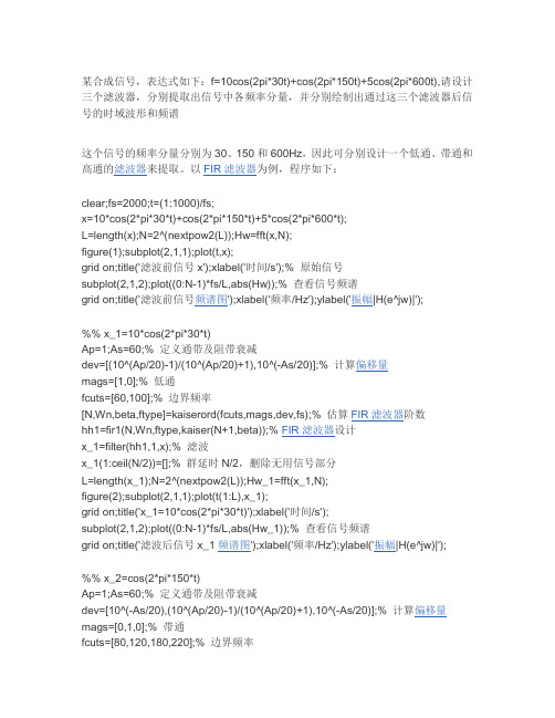
某合成信号,表达式如下:f=10cos(2pi*30t)+cos(2pi*150t)+5cos(2pi*600t),请设计三个滤波器,分别提取出信号中各频率分量,并分别绘制出通过这三个滤波器后信号的时域波形和频谱这个信号的频率分量分别为30、150和600Hz,因此可分别设计一个低通、带通和高通的滤波器来提取。
以FIR滤波器为例,程序如下:clear;fs=2000;t=(1:1000)/fs;x=10*cos(2*pi*30*t)+cos(2*pi*150*t)+5*cos(2*pi*600*t);L=length(x);N=2^(nextpow2(L));Hw=fft(x,N);figure(1);subplot(2,1,1);plot(t,x);grid on;title('滤波前信号x');xlabel('时间/s');% 原始信号subplot(2,1,2);plot((0:N-1)*fs/L,abs(Hw));% 查看信号频谱grid on;title('滤波前信号频谱图');xlabel('频率/Hz');ylabel('振幅|H(e^jw)|');%% x_1=10*cos(2*pi*30*t)Ap=1;As=60;% 定义通带及阻带衰减dev=[(10^(Ap/20)-1)/(10^(Ap/20)+1),10^(-As/20)];% 计算偏移量mags=[1,0];% 低通fcuts=[60,100];% 边界频率[N,Wn,beta,ftype]=kaiserord(fcuts,mags,dev,fs);% 估算FIR滤波器阶数hh1=fir1(N,Wn,ftype,kaiser(N+1,beta));% FIR滤波器设计x_1=filter(hh1,1,x);% 滤波x_1(1:ceil(N/2))=[];% 群延时N/2,删除无用信号部分L=length(x_1);N=2^(nextpow2(L));Hw_1=fft(x_1,N);figure(2);subplot(2,1,1);plot(t(1:L),x_1);grid on;title('x_1=10*cos(2*pi*30*t)');xlabel('时间/s');subplot(2,1,2);plot((0:N-1)*fs/L,abs(Hw_1));% 查看信号频谱grid on;title('滤波后信号x_1频谱图');xlabel('频率/Hz');ylabel('振幅|H(e^jw)|');%% x_2=cos(2*pi*150*t)Ap=1;As=60;% 定义通带及阻带衰减dev=[10^(-As/20),(10^(Ap/20)-1)/(10^(Ap/20)+1),10^(-As/20)];% 计算偏移量mags=[0,1,0];% 带通fcuts=[80,120,180,220];% 边界频率[N,Wn,beta,ftype]=kaiserord(fcuts,mags,dev,fs);% 估算FIR滤波器阶数hh2=fir1(N,Wn,ftype,kaiser(N+1,beta));% FIR滤波器设计x_2=filter(hh2,1,x);% 滤波x_2(1:ceil(N/2))=[];% 群延时N/2,删除无用信号部分L=length(x_2);N=2^(nextpow2(L));Hw_2=fft(x_2,N);figure(3);subplot(2,1,1);plot(t(1:L),x_2);grid on;title('x_2=cos(2*pi*150*t)');xlabel('时间/s');subplot(2,1,2);plot((0:N-1)*fs/L,abs(Hw_2));% 查看信号频谱grid on;title('滤波后信号x_2频谱图');xlabel('频率/Hz');ylabel('振幅|H(e^jw)|');%% x_3=5*cos(2*pi*600*t)Ap=1;As=60;% 定义通带及阻带衰减dev=[10^(-As/20),(10^(Ap/20)-1)/(10^(Ap/20)+1)];% 计算偏移量mags=[0,1];% 高通fcuts=[500,550];% 边界频率[N,Wn,beta,ftype]=kaiserord(fcuts,mags,dev,fs);% 估算FIR滤波器阶数hh2=fir1(N,Wn,ftype,kaiser(N+1,beta));% FIR滤波器设计x_3=filter(hh2,1,x);% 滤波x_3(1:ceil(N/2))=[];% 群延时N/2,删除无用信号部分L=length(x_3);N=2^(nextpow2(L));Hw_3=fft(x_3,N);figure(4);subplot(2,1,1);plot(t(1:L),x_3);grid on;title('x_3=5*cos(2*pi*600*t)');xlabel('时间/s');subplot(2,1,2);plot((0:N-1)*fs/L,abs(Hw_3));% 查看信号频谱grid on;title('滤波后信号x_3频谱图');xlabel('频率/Hz');ylabel('振幅|H(e^jw)|');。
matlab 粒子滤波代码
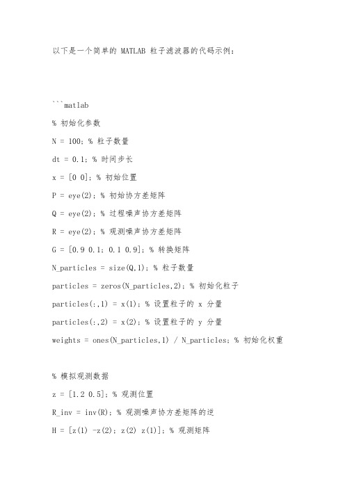
以下是一个简单的 MATLAB 粒子滤波器的代码示例:```matlab% 初始化参数N = 100; % 粒子数量dt = 0.1; % 时间步长x = [0 0]; % 初始位置P = eye(2); % 初始协方差矩阵Q = eye(2); % 过程噪声协方差矩阵R = eye(2); % 观测噪声协方差矩阵G = [0.9 0.1; 0.1 0.9]; % 转换矩阵N_particles = size(Q,1); % 粒子数量particles = zeros(N_particles,2); % 初始化粒子particles(:,1) = x(1); % 设置粒子的 x 分量particles(:,2) = x(2); % 设置粒子的 y 分量weights = ones(N_particles,1) / N_particles; % 初始化权重% 模拟观测数据z = [1.2 0.5]; % 观测位置R_inv = inv(R); % 观测噪声协方差矩阵的逆H = [z(1) -z(2); z(2) z(1)]; % 观测矩阵y = H * x; % 预测的观测值% 粒子滤波步骤for t = 1:100% 重采样步骤weights = weights / sum(weights);index = randsample(1:N_particles, N, true, weights); particles = particles(index,:);% 预测步骤x_pred = particles;P_pred = Q;x_pred = G * x_pred;P_pred = P_pred + dt * G * P_pred;P_pred = P_pred + P_pred * G' + R;% 更新步骤y_pred = H * x_pred;S = H * P_pred * H' + R_inv;K = P_pred * H' * inv(S);x = x_pred + K * (z - y_pred);P = P_pred - P_pred * K * H';end```在这个代码示例中,我们使用了两个步骤:重采样步骤和预测/更新步骤。
matlab滤波器代码要点

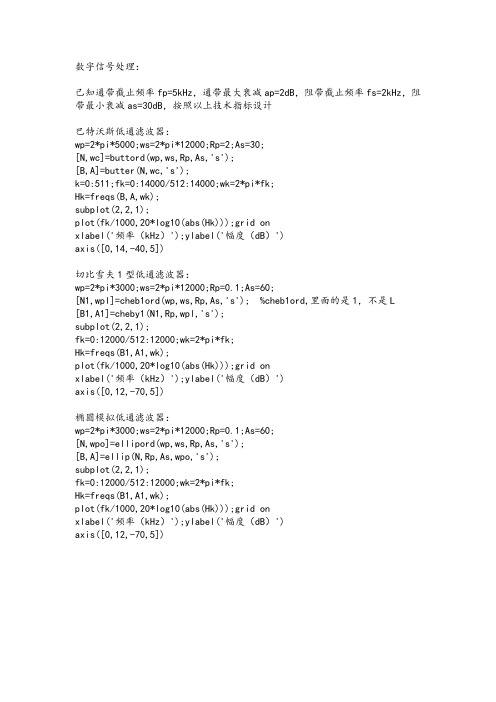
数字信号处理:已知通带截止频率fp=5kHz,通带最大衰减ap=2dB,阻带截止频率fs=2kHz,阻带最小衰减as=30dB,按照以上技术指标设计巴特沃斯低通滤波器:wp=2*pi*5000;ws=2*pi*12000;Rp=2;As=30;[N,wc]=buttord(wp,ws,Rp,As,'s');[B,A]=butter(N,wc,'s');k=0:511;fk=0:14000/512:14000;wk=2*pi*fk;Hk=freqs(B,A,wk);subplot(2,2,1);plot(fk/1000,20*log10(abs(Hk)));grid onxlabel('频率(kHz)');ylabel('幅度(dB)')axis([0,14,-40,5])切比雪夫1型低通滤波器:wp=2*pi*3000;ws=2*pi*12000;Rp=0.1;As=60;[N1,wpl]=cheb1ord(wp,ws,Rp,As,'s'); %cheb1ord,里面的是1,不是L[B1,A1]=cheby1(N1,Rp,wpl,'s');subplot(2,2,1);fk=0:12000/512:12000;wk=2*pi*fk;Hk=freqs(B1,A1,wk);plot(fk/1000,20*log10(abs(Hk)));grid onxlabel('频率(kHz)');ylabel('幅度(dB)')axis([0,12,-70,5])椭圆模拟低通滤波器:wp=2*pi*3000;ws=2*pi*12000;Rp=0.1;As=60;[N,wpo]=ellipord(wp,ws,Rp,As,'s');[B,A]=ellip(N,Rp,As,wpo,'s');subplot(2,2,1);fk=0:12000/512:12000;wk=2*pi*fk;Hk=freqs(B1,A1,wk);plot(fk/1000,20*log10(abs(Hk)));grid onxlabel('频率(kHz)');ylabel('幅度(dB)')axis([0,12,-70,5])p195-14wp=2*4/80;ws=2*20/80;rp=0.5;rs=45;[N,wc]=buttord(wp,ws,rp,rs);[B,A]=butter(N,wc);[hk,wk]=freqz(B,A);fk=wk/pi*40;plot(fk,20*log10(abs(hk)));axis([0,30,-100,0])xlabel('频率(kHZ)');ylabel('幅度(db)');grid on P195-16wp=2*325/2500;ws=2*225/2500;rp=1;rs=40;[N,wc]=ellipord(wp,ws,rp,rs);[B,A]=ellip(N,rp,rs,wc);[hk,wk]=freqz(B,A);fk=wk/pi*40;plot(fk,20*log10(abs(hk)));axis([0,30,-100,0])xlabel('频率(kHZ)');ylabel('幅度(db)');grid onP195-15wp=2*4/80;ws=2*20/80;rp=0.5;rs=45;[N,wc]=cheb1ord(wp,ws,rp,rs);[B,A]=cheby1(N,rp,wc);[hk,wk]=freqz(B,A);fk=wk/pi*40;plot(fk,20*log10(abs(hk)));axis([0,30,-100,0])xlabel('频率(kHZ)');ylabel('幅度(db)');grid on 切比雪夫低通滤波器wp=2*pi*3000;ws=2*pi*12000;rp=0.1;as=60;[N1,wp1]=cheb1ord(wp,ws,rp,as,'s');[B1,A1]=cheby1(N1,rp,wp1,'s');subplot(2,2,1);fk=0:12000/512:12000;wk=2*pi*fk;hk=freqs(B1,A1,wk);plot(fk/1000,20*log10(abs(hk)));grid onxlabel('频率(kHZ)');ylabel('幅度(db)');axis([0,12,-70,5])双音频检测audiofile='test.wav'[in_audio,fs,bits]=wavread(audiofile); [b,a]=cheby1(5,0.1,0.3);out_audio=filter(b,a,in_audio);sound(out_audio,fs,bits);wavwrite(out_audio,fs,bits,'test_out'); xk1=fft(in_audio,512);xk2=fft(out_audio,512);subplot(2,1,1);stem(abs(xk1));subplot(2,1,2);stem(abs(xk2));巴特沃斯模拟高通滤波器。
粒子滤波算法matlab实例
一、介绍粒子滤波算法粒子滤波算法是一种基于蒙特卡洛方法的非线性、非高斯滤波算法,它通过一组随机产生的粒子来近似表示系统的后验概率分布,从而实现对非线性、非高斯系统的状态估计。
在实际应用中,粒子滤波算法被广泛应用于目标跟踪、导航、机器人定位等领域。
本文将以matlab 实例的形式介绍粒子滤波算法的基本原理和应用。
二、粒子滤波算法的原理及步骤粒子滤波算法的主要原理是基于贝叶斯滤波理论,通过一组随机产生的粒子来近似表示系统的后验概率分布。
其具体步骤如下:1. 初始化:随机生成一组粒子,对于状态变量的初始值和方差的估计,通过随机抽样得到一组粒子。
2. 预测:根据系统模型,对每个粒子进行状态预测,得到预测状态。
3. 更新:根据测量信息,对每个预测状态进行权重更新,得到更新后的状态。
4. 重采样:根据更新后的权重,对粒子进行重采样,以满足后验概率分布的表示。
5. 输出:根据重采样后的粒子,得到对系统状态的估计。
三、粒子滤波算法的matlab实例下面以一个简单的目标跟踪问题为例,介绍粒子滤波算法在matlab中的实现。
假设存在一个目标在二维空间中运动,我们需要通过一系列测量得到目标的状态。
我们初始化一组粒子来近似表示目标的状态分布。
我们根据目标的运动模型,预测每个粒子的状态。
根据测量信息,对每个预测状态进行权重更新。
根据更新后的权重,对粒子进行重采样,并输出对目标状态的估计。
在matlab中,我们可以通过编写一段简单的代码来实现粒子滤波算法。
我们需要定义目标的运动模型和测量模型,然后初始化一组粒子。
我们通过循环来进行预测、更新、重采样的步骤,最终得到目标状态的估计。
四、总结粒子滤波算法是一种非线性、非高斯滤波算法,通过一组随机产生的粒子来近似表示系统的后验概率分布。
在实际应用中,粒子滤波算法被广泛应用于目标跟踪、导航、机器人定位等领域。
本文以matlab实例的形式介绍了粒子滤波算法的基本原理和应用,并通过一个简单的目标跟踪问题,展示了粒子滤波算法在matlab中的实现过程。
matlab滤波器代码
数字信号处理:已知通带截止频率fp=5kHz,通带最大衰减ap=2dB,阻带截止频率fs=2kHz,阻带最小衰减as=30dB,按照以上技术指标设计巴特沃斯低通滤波器:wp=2*pi*5000;ws=2*pi*12000;Rp=2;As=30;[N,wc]=buttord(wp,ws,Rp,As,'s');[B,A]=butter(N,wc,'s');k=0:511;fk=0:14000/512:14000;wk=2*pi*fk;Hk=freqs(B,A,wk);subplot(2,2,1);plot(fk/1000,20*log10(abs(Hk)));grid onxlabel('频率(kHz)');ylabel('幅度(dB)')axis([0,14,-40,5])切比雪夫1型低通滤波器:wp=2*pi*3000;ws=2*pi*12000;Rp=0.1;As=60;[N1,wpl]=cheb1ord(wp,ws,Rp,As,'s');%cheb1ord,里面的是1,不是L[B1,A1]=cheby1(N1,Rp,wpl,'s');subplot(2,2,1);fk=0:12000/512:12000;wk=2*pi*fk;Hk=freqs(B1,A1,wk);plot(fk/1000,20*log10(abs(Hk)));grid onxlabel('频率(kHz)');ylabel('幅度(dB)')axis([0,12,-70,5])椭圆模拟低通滤波器:wp=2*pi*3000;ws=2*pi*12000;Rp=0.1;As=60;[N,wpo]=ellipord(wp,ws,Rp,As,'s');[B,A]=ellip(N,Rp,As,wpo,'s');subplot(2,2,1);fk=0:12000/512:12000;wk=2*pi*fk;Hk=freqs(B1,A1,wk);plot(fk/1000,20*log10(abs(Hk)));grid onxlabel('频率(kHz)');ylabel('幅度(dB)')axis([0,12,-70,5])p195-14wp=2*4/80;ws=2*20/80;rp=0.5;rs=45;[N,wc]=buttord(wp,ws,rp,rs);[B,A]=butter(N,wc);[hk,wk]=freqz(B,A);fk=wk/pi*40;plot(fk,20*log10(abs(hk)));axis([0,30,-100,0])xlabel('频率(kHZ)');ylabel('幅度(db)');grid on P195-16wp=2*325/2500;ws=2*225/2500;rp=1;rs=40;[N,wc]=ellipord(wp,ws,rp,rs);[B,A]=ellip(N,rp,rs,wc);[hk,wk]=freqz(B,A);fk=wk/pi*40;plot(fk,20*log10(abs(hk)));axis([0,30,-100,0])xlabel('频率(kHZ)');ylabel('幅度(db)');grid onP195-15wp=2*4/80;ws=2*20/80;rp=0.5;rs=45;[N,wc]=cheb1ord(wp,ws,rp,rs);[B,A]=cheby1(N,rp,wc);[hk,wk]=freqz(B,A);fk=wk/pi*40;plot(fk,20*log10(abs(hk)));axis([0,30,-100,0])xlabel('频率(kHZ)');ylabel('幅度(db)');grid on 切比雪夫低通滤波器wp=2*pi*3000;ws=2*pi*12000;rp=0.1;as=60;[N1,wp1]=cheb1ord(wp,ws,rp,as,'s');[B1,A1]=cheby1(N1,rp,wp1,'s');subplot(2,2,1);fk=0:12000/512:12000;wk=2*pi*fk;hk=freqs(B1,A1,wk);plot(fk/1000,20*log10(abs(hk)));grid onxlabel('频率(kHZ)');ylabel('幅度(db)');axis([0,12,-70,5])双音频检测audiofile='test.wav'[in_audio,fs,bits]=wavread(audiofile); [b,a]=cheby1(5,0.1,0.3);out_audio=filter(b,a,in_audio);sound(out_audio,fs,bits);wavwrite(out_audio,fs,bits,'test_out'); xk1=fft(in_audio,512);xk2=fft(out_audio,512);subplot(2,1,1);stem(abs(xk1));subplot(2,1,2);stem(abs(xk2));巴特沃斯模拟高通滤波器。
pf算法举例及其matlab实现-概述说明以及解释
pf算法举例及其matlab实现-概述说明以及解释1.引言1.1 概述PF算法(Particle Filter Algorithm),又称为粒子滤波算法,是一种基于蒙特卡洛方法的非线性滤波算法。
与传统的滤波算法相比,PF算法具有更大的灵活性和鲁棒性,在估计复杂非线性系统状态的过程中表现出良好的性能。
PF算法基于一种随机采样的思想,通过对系统状态进行一系列粒子的采样,再通过对这些粒子的权重进行重要性重采样,最终获得对状态估计的准确性更高的结果。
在PF算法中,粒子的数量决定了滤波算法的精度,粒子越多,估计结果越准确,但也会增加计算复杂度。
因此,在实际应用中需要根据实际情况灵活选择粒子数量。
作为一种高效的滤波算法,PF算法在众多领域都有广泛的应用。
例如,粒子滤波算法在目标跟踪、传感器网络定位、机器人定位与导航等领域都有着重要的作用。
其在目标跟踪领域的应用尤为突出,由于PF算法可以处理非线性和非高斯分布的情况,使得目标跟踪更加准确和稳定。
在Matlab中,PF算法也得到了广泛的应用和实现。
Matlab提供了丰富的函数和工具箱,可以便捷地实现PF算法。
借助Matlab的强大数据处理和可视化功能,我们可以更加便捷地进行粒子滤波算法的实现和结果分析。
本文将从PF算法的基本概念出发,介绍其应用举例和在Matlab中的具体实现。
通过对PF算法的研究和实践,我们可以更好地理解和应用这一强大的滤波算法,为实际问题的解决提供有效的手段。
通过对Matlab 的使用,我们还可以更加高效地实现和验证粒子滤波算法的性能,为进一步的研究和应用奠定基础。
在接下来的章节中,我们将详细介绍PF算法的原理及其在现实应用中的具体案例。
随后,我们将展示如何使用Matlab实现PF算法,并通过实验结果对其性能进行评估和分析。
最后,我们将总结PF算法和Matlab 实现的主要特点,并对未来的发展进行展望。
文章结构的设定在撰写一篇长文时非常重要,它能够为读者提供一个整体的概览,帮助他们更好地理解文章的内容安排。
在MATLAB中使用粒子滤波进行状态估计
在MATLAB中使用粒子滤波进行状态估计Introduction:在许多实时系统或者控制系统中,状态估计是至关重要的一环。
状态估计涉及通过测量数据来推断或估计系统的当前状态。
而粒子滤波(Particle filter)作为一种无模型非线性滤波器,被广泛应用于状态估计问题中。
在本文中,我们将重点介绍如何在MATLAB中使用粒子滤波进行状态估计。
Particle filter基本原理:粒子滤波基于贝叶斯滤波理论,并通过一系列随机样本表示系统的可能状态。
它的基本原理是通过一个粒子集合来近似表示系统状态的概率密度函数。
粒子滤波的核心思想是通过对每个状态进行加权采样来逼近概率密度函数。
粒子的数量越多,逼近的精度就越高,但同时计算量也会增加。
在粒子滤波算法中,每个粒子表示系统的一个假设状态,粒子的权重表示此假设状态的似然度。
而粒子的更新则通过重采样和预测两个步骤来实现。
重采样过程会根据粒子的权重来决定哪些粒子要留下来,而预测过程则通过系统动力学方程来生成新的粒子。
在状态估计问题中,粒子滤波可以通过将传感器测量数据与系统模型相结合,来估计系统的状态。
在MATLAB中使用粒子滤波:使用MATLAB进行粒子滤波非常方便,因为MATLAB提供了强大的工具箱和函数来支持粒子滤波算法,比如Statistics and Machine Learning Toolbox和Sensor Fusion and Tracking Toolbox。
在这里,我们将使用Statistics and Machine Learning Toolbox来进行演示。
步骤一: 初始化粒子集合首先,我们需要根据系统的先验信息,生成一组初始化的粒子。
我们可以根据先验概率密度函数来对粒子赋初值。
```MATLABnumParticles = 1000; % 粒子的数量particleSet = rand(numParticles, 2); % 初始化粒子集合```步骤二: 测量更新接下来,我们需要使用传感器测量数据来对粒子进行加权更新。
粒子滤波PF算法在无线传感器网络定位跟踪的matlab源码
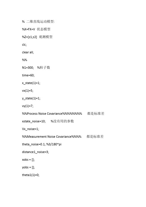
% 二维直线运动模型:%X=FX+V 状态模型%Z=[z1;z2] 观测模型clc;clear all;%%N1=300; %粒子数time=60;x_state(1)=1;vx(1)=5;y_state(1)=1;vy(1)=7;%%Process Noise Covariance%%%%%%%% 都是标准差xstate_noise=10; %没有用的参数Vx_noise=1;%%Measurement Noise Covariance%%%% 都是标准差theta_noise=0.1; %3/180*pidistance1_noise=3;xobs = [];yobs = [];theta1(1)=0;%%Ture State%%%%%%%%for i=2:time%% State model%%%%%%%%%%%accx = normrnd(0,Vx_noise,1,1);x_state(i)=x_state(i-1)+vx(i-1)+0.5*accx;vx(i)=vx(i-1)+accx;accy = normrnd(0,Vx_noise,1,1);y_state(i)=y_state(i-1)+vy(i-1)+0.5*accy;vy(i)=vy(i-1)+accy;end%%Measurement Value%%%%%for i=1:time%%Measure model%%%%%%%%%distance1(i)=sqrt(x_state(i)^2+y_state(i)^2)+distance1_noise*randn(1);%theta1(i)=atan(y_state(i)/x_state(i))+theta_noise*randn(1);%使用下面增加了象限判断的角度计算方式[-pi,pi]if x_state(i)>0 && y_state(i)>=0theta1(i) = atan(y_state(i)/x_state(i))+theta_noise*randn(1) ; %观测方程endif x_state(i)<0 && y_state(i)>=0theta1(i) = (atan(y_state(i)/x_state(i))+pi) +theta_noise*randn(1); %观测方程endif x_state(i)<0 && y_state(i)<=0theta1(i) = (atan(y_state(i)/x_state(i))-pi) +theta_noise*randn(1); %观测方程endif x_state(i)>0 && y_state(i)<=0theta1(i) = atan(y_state(i)/x_state(i)) +theta_noise*randn(1); %观测方程endxobs = [xobs distance1(i)*cos(theta1(i))];yobs = [yobs distance1(i)*sin(theta1(i))];end%%%Particle Filtering%%%%%%%%%%%%%%x_pf(1)=x_state(1);vx_pf(1)=vx(1);y_pf(1)=y_state(1);vy_pf(1)=vy(1);xp1=zeros(1,N1);xp2=zeros(1,N1);xp3=zeros(1,N1);xp4=zeros(1,N1); %%%%%Initial particles 得到初始化的粒子群%%%%%%%%for n=1:N1;%M1=[delta1*randn(1),delta2*randn(1),delta3*randn(1),delta4*randn(1)];%M1=diag(M1);xp1(n)=x_pf(1)+normrnd(0,Vx_noise,1,1);xp2(n)=vx_pf(1)+normrnd(0,Vx_noise,1,1);xp3(n)=y_pf(1)+normrnd(0,Vx_noise,1,1);xp4(n)=vy_pf(1)+normrnd(0,Vx_noise,1,1);end%**filter process*** angel and distance**************** for t=2:time%%%Prediction Process%%%%for n=1:N1accx = normrnd(0,Vx_noise,1,1);xpre_pf(n)=xp1(n)+xp2(n)+0.5*accx;vxpre_pf(n)=xp2(n)+accx;accy = normrnd(0,Vx_noise,1,1);ypre_pf(n)=xp3(n)+xp4(n)+0.5*accy;vypre_pf(n)=xp4(n)+accy;end%%%Calculate Weight Particles%%%%for n=1:N1vhat1=sqrt(xpre_pf(n)^2+ypre_pf(n)^2)-distance1(t);%vhat2=atan(ypre_pf(n)/xpre_pf(n))-theta1(t);%使用下面增加了象限判断的角度计算方式if xpre_pf(n)>0 && ypre_pf(n)>=0ag = atan(ypre_pf(n)/xpre_pf(n)) ; %观测方程endif xpre_pf(n)<0 && ypre_pf(n)>=0ag = (atan(ypre_pf(n)/xpre_pf(n))+pi); %观测方程endif xpre_pf(n)<0 && ypre_pf(n)<=0ag = (atan(ypre_pf(n)/xpre_pf(n))-pi) ; %观测方程endif xpre_pf(n)>0 && ypre_pf(n)<=0ag = atan(ypre_pf(n)/xpre_pf(n)); %观测方程endvhat2=ag-theta1(t);q1=(1/distance1_noise/sqrt(2*pi))*exp(-vhat1^2/2/distance1_noise^2);q2=(1/theta_noise/sqrt(2*pi))*exp(-vhat2^2/2/theta_noise^2);q(n)=q1*q2+1e-99;endq = q./sum(q);P_pf = cumsum(q);%%Resampling Process 这是一种均匀的重采样方法,随机数的产生不再是从[0,1]上任意产生,而是使这个随机数渐进式的增大,与权重累加和一样,都是交替上升,这样的比较更有规律性,更周到%%%%%%%%%%%%%%ut(1)=rand(1)/N1;k = 1;hp = zeros(1,N1);for j = 1:N1ut(j)=ut(1)+(j-1)/N1;while(P_pf(k)<ut(j));k = k + 1;end;hp(j) = k;q(j)=1/N1;end;xp1 = xpre_pf(hp); xp2 = vxpre_pf(hp); % The new particles xp3 = ypre_pf(hp); xp4 = vypre_pf(hp);%% Compute the estimate%%%%%%%%%%%%%x_pf(t)=mean(xp1);y_pf(t)=mean(xp3);end%%%%Result of Tracking%%%%%%%%%%%%% figure;plot(x_state,y_state,'r-*',x_pf,y_pf,'b-o',xobs,yobs,'g-d') xlabel('x state'); ylabel('y state');legend('实际轨迹','滤波轨迹','观测轨迹');set(gcf,'Color','White');%figure;%plot(1:time,distance_error,'r');%legend('distance error');。
- 1、下载文档前请自行甄别文档内容的完整性,平台不提供额外的编辑、内容补充、找答案等附加服务。
- 2、"仅部分预览"的文档,不可在线预览部分如存在完整性等问题,可反馈申请退款(可完整预览的文档不适用该条件!)。
- 3、如文档侵犯您的权益,请联系客服反馈,我们会尽快为您处理(人工客服工作时间:9:00-18:30)。
function ParticleEx1
% Particle filter example, adapted from Gordon, Salmond, and Smith paper.
x = 0.1; % initial state
Q = 1; % process noise covariance
R = 1; % measurement noise covariance
tf = 50; % simulation length
N = 100; % number of particles in the particle filter
xhat = x;
P = 2;
xhatPart = x;
% Initialize the particle filter.
for i = 1 : N
xpart(i) = x + sqrt(P) * randn;
end
jArr = [0];
xArr = [x];
yArr = [x^2 / 20 + sqrt(R) * randn];
xhatArr = [x];
PArr = [P];
xhatPartArr = [xhatPart];
close all;
for k = 1 : tf
% System simulation
x = 0.5 * x + 25 * x / (1 + x^2) + 8 * cos(1.2*(k-1)) + sqrt(Q) * randn;%状态方程
y = x^2 / 20 + sqrt(R) * randn;%观测方程
% Extended Kalman filter
F = 0.5 + 25 * (1 - xhat^2) / (1 + xhat^2)^2;
P = F * P * F' + Q;
H = xhat / 10;
K = P * H' * (H * P * H' + R)^(-1);
xhat = 0.5 * xhat + 25 * xhat / (1 + xhat^2) + 8 * cos(1.2*(k-1));%预测
xhat = xhat + K * (y - xhat^2 / 20);%更新
P = (1 - K * H) * P;
% Particle filter
for i = 1 : N
xpartminus(i) = 0.5 * xpart(i) + 25 * xpart(i) / (1 + xpart(i)^2) + 8 * cos(1.2*(k-1)) + sqrt(Q) * randn;
ypart = xpartminus(i)^2 / 20;
vhat = y - ypart;%观测和预测的差
q(i) = (1 / sqrt(R) / sqrt(2*pi)) * exp(-vhat^2 / 2 / R);
end
% Normalize the likelihood of each a priori estimate.
qsum = sum(q);
for i = 1 : N
q(i) = q(i) / qsum;%归一化权重
end
% Resample.重采样
for i = 1 : N
u = rand; % uniform random number between 0 and 1
qtempsum = 0;
for j = 1 : N
qtempsum = qtempsum + q(j);
if qtempsum >= u
xpart(i) = xpartminus(j);
if k == 20
qArr=q;
jArr = [jArr j];
end
break;
end
end
end
% The particle filter estimate is the mean of the particles.
xhatPart = mean(xpart);
% Plot the estimated pdf's at a specific time.
if k == 20
% Particle filter pdf
pdf = zeros(81,1);
for m = -40 : 40
for i = 1 : N
if (m <= xpart(i)) && (xpart(i) < m+1)
pdf(m+41) = pdf(m+41) + 1;
end
end
end
figure;
m = -40 : 40;
plot(m, pdf / N, 'r');
hold;
title('Estimated pdf at k=20');
disp(['min, max xpart(i) at k = 20: ', num2str(min(xpart)), ', ', num2str(max(xpart))]);
% Kalman filter pdf
pdf = (1 / sqrt(P) / sqrt(2*pi)) .* exp(-(m - xhat).^2 / 2 / P);
plot(m, pdf, 'b');
legend('Particle filter', 'Kalman filter');
grid on;
end
% Save data in arrays for later plotting
xArr = [xArr x];
yArr = [yArr y];
xhatArr = [xhatArr xhat];
PArr = [PArr P];
xhatPartArr = [xhatPartArr xhatPart];
end
t = 0 : tf;
%figure;
%plot(t, xArr);
%ylabel('true state');
figure;
plot(t, xArr, 'b.', t, xhatArr, 'g-.', t, xhatArr-2*sqrt(PArr), 'r:', t, xhatArr+2*sqrt(PArr), 'r:'); axis([0 tf -40 40]);
set(gca,'FontSize',12); set(gcf,'Color','White');
xlabel('time step'); ylabel('state');
legend('True state', 'EKF estimate', '95% confidence region');
grid on;
figure;
plot(t, xArr, 'b.', t, xhatPartArr, 'k-');
set(gca,'FontSize',12); set(gcf,'Color','White');
xlabel('time step'); ylabel('state');
legend('True state', 'Particle filter estimate');
grid on;
xhatRMS = sqrt((norm(xArr - xhatArr))^2 / tf);
xhatPartRMS = sqrt((norm(xArr - xhatPartArr))^2 / tf);
disp(['Kalman filter RMS error = ', num2str(xhatRMS)]);
disp(['Particle filter RMS error = ', num2str(xhatPartRMS)]);
/*qArr
tt=max(qArr)
t=jArr
[m,n]=hist(jArr,100)
m
n
sum(m) 完!。