实验指导书(ARIMA模型建模与预测)
实验一 arima模型建立与应用.doc

实验一 ARIMA 模型建立与应用一、实验项目:ARIMA 模型建立与预测。
二、实验目的1、准确掌握ARIMA(p,d,q)模型各种形式和基本原理;2、熟练识别ARIMA(p,d,q)模型中的阶数p,d,q 的方法;3、学会建立及检验ARIMA(p,d,q)模型的方法;4、熟练掌握运用ARIMA(p,d,q)模型对样本序列进行拟合和预测; 三、预备知识(一)模型1、AR (p )(p 阶自回归模型)t p t p t t t u x x x x +++++=---φφφδ 2211其中u t 白噪声序列,δ是常数(表示序列数据没有0均值化) AR (p )等价于t t p p u x L L L +=----δφφφ)1(221AR (p )的特征方程是:01)(221=----=Φp p L L L L φφφ AR (p )平稳的充要条件是特征根都在单位圆之外。
2、MA (q )(q 阶移动平均模型)q t q t t t t u u u u x ---+++++=θθθμ 2211t t q q t u L u L L L x )()1(221Θ=++++=-θθθμ其中{u t }是白噪声过程。
MA (q )平稳性MA (q )是由u t 本身和q 个u t 的滞后项加权平均构造出来的,因此它是平稳的。
MA (q )可逆性(用自回归序列表示u t )t t x L u 1)]([-Θ=可逆条件:即1)]([-ΘL 收敛的条件。
即Θ(L )每个特征根绝对值大于1,即全部特征根在单位圆之外。
3、ARMA (p ,q )(自回归移动平均过程)q t q t t t p t p t t t u u u u x x x x ------+++++++++=θθθδφφφ 22112211t t qq tp p t u L u L L L x L L L x L )()1()1()(221221Θ+=+++++=----=Φδθθθδφφφt t u L x L )()(Θ+=ΦδARMA (p ,q )平稳性的条件是方程Φ(L )=0的根都在单位圆外;可逆性条件是方程Θ(L )=0的根全部在单位圆外。
VR虚拟现实-实验一 ARIMA模型建立与应用 精品
实验一 ARIMA 模型建立与应用一、实验项目:ARIMA 模型建立与预测。
二、实验目的1、准确掌握ARIMA(p,d,q)模型各种形式和基本原理;2、熟练识别ARIMA(p,d,q)模型中的阶数p,d,q 的方法;3、学会建立及检验ARIMA(p,d,q)模型的方法;4、熟练掌握运用ARIMA(p,d,q)模型对样本序列进行拟合和预测; 三、预备知识(一)模型1、AR (p )(p 阶自回归模型)t p t p t t t u x x x x +++++=---φφφδ 2211其中u t 白噪声序列,δ是常数(表示序列数据没有0均值化) AR (p )等价于t t p p u x L L L +=----δφφφ)1(221AR (p )的特征方程是:01)(221=----=Φp p L L L L φφφ AR (p )平稳的充要条件是特征根都在单位圆之外。
2、MA (q )(q 阶移动平均模型)q t q t t t t u u u u x ---+++++=θθθμ 2211t t q q t u L u L L L x )()1(221Θ=++++=-θθθμ其中{u t }是白噪声过程。
MA (q )平稳性MA (q )是由u t 本身和q 个u t 的滞后项加权平均构造出来的,因此它是平稳的。
MA (q )可逆性(用自回归序列表示u t )t t x L u 1)]([-Θ=可逆条件:即1)]([-ΘL 收敛的条件。
即Θ(L )每个特征根绝对值大于1,即全部特征根在单位圆之外。
3、ARMA (p ,q )(自回归移动平均过程)q t q t t t p t p t t t u u u u x x x x ------+++++++++=θθθδφφφ 22112211t t qq tp p t u L u L L L x L L L x L )()1()1()(221221Θ+=+++++=----=Φδθθθδφφφt t u L x L )()(Θ+=ΦδARMA (p ,q )平稳性的条件是方程Φ(L )=0的根都在单位圆外;可逆性条件是方程Θ(L )=0的根全部在单位圆外。
实验指导书(ARIMA模型建模与预测)
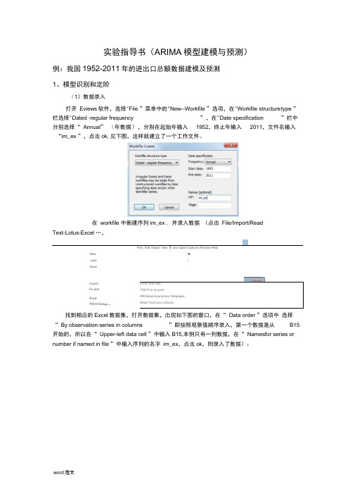
实验指导书(ARIMA 模型建模与预测)例:我国1952-2011年的进出口总额数据建模及预测1、模型识别和定阶(1)数据录入打开 Eviews 软件,选择"File ”菜单中的"New--Workfile ”选项,在"Workfile structure type ”栏选择"Dated -regular frequency”,在"Date specification”栏中分别选择“ Annual ” (年数据),分别在起始年输入 1952,终止年输入 2011,文件名输入 “im_ex ”,点击ok ,见下图,这样就建立了一个工作文件。
在 workfile 中新建序列im_ex , 并录入数据 (点击 File/Import/ReadText-Lotus-Excel …,File | Edit Object View 卩iroc Quick Options Window HelpNew ► □pen iSaveFetch from DB... T5D Fi le Im port-.DRI Bask Economics Database... Read Text-Lctu s-Excel...找到相应的Excel 数据集,打开数据集,出现如下图的窗口,在“ Data order ”选项中 选择“ By observation-series in columns”即按照观察值顺序录入,第一个数据是从B15开始的,所以在“ Upper-left data cell ”中输入B15,本例只有一列数据,在“ Namesfor series or number if named in file ”中输入序列的名字 im_ex ,点击ok ,则录入了数据):import Ex port PrintPtFrtl Setup-.,.Excel Spreadthtei Import —JData orderQ By Obssrvalkn「senes h cokums目Y Scries - series in rowiUpper^eft daiacefl Excd 5 4 sheet name Names for scries or Nuniw if named in fteIHIJK IinCKKt sample 1952 2D 11""I Write dak/ote 曰髓比$ H申烧1和rm审tFrst caiiendar dayLast Qtendsr day■Vrltfi senes namesReset iflEpk to:O Current sample-Q WafkHe rangeQ To md af rangeOK | Cwictl(2) 时序图判断平稳性双击序列im_ex,点击view/Graph/line ,得到下列对话框:显著非平稳。
实验三:ARIMA模型建模与预测实验报告

课程论文(2016 / 2017学年第 1 学期)课程名称应用时间序列分析指导单位经济学院指导教师易莹莹学生姓名班级学号学院(系) 经济学院专业经济统计学实验三ARIMA 模型建模与预测实验指导一、实验目的:了解ARIMA 模型的特点和建模过程,了解AR ,MA 和ARIMA 模型三者之间的区别与联系,掌握如何利用自相关系数和偏自相关系数对ARIMA 模型进行识别,利用最小二乘法等方法对ARIMA 模型进行估计,利用信息准则对估计的ARIMA 模型进行诊断,以及如何利用ARIMA 模型进行预测。
掌握在实证研究如何运用Eviews 软件进行ARIMA 模型的识别、诊断、估计和预测。
二、基本概念:所谓ARIMA 模型,是指将非平稳时间序列转化为平稳时间序列,然后将平稳的时间序列建立ARMA 模型。
ARIMA 模型根据原序列是否平稳以及回归中所含部分的不同,包括移动平均过程(MA )、自回归过程(AR )、自回归移动平均过程(ARMA )以及ARIMA 过程。
在ARIMA 模型的识别过程中,我们主要用到两个工具:自相关函数ACF ,偏自相关函数PACF 以及它们各自的相关图。
对于一个序列{}t X 而言,它的第j 阶自相关系数j ρ为它的j 阶自协方差除以方差,即j ρ=j 0γγ,它是关于滞后期j 的函数,因此我们也称之为自相关函数,通常记ACF(j )。
偏自相关函数PACF(j )度量了消除中间滞后项影响后两滞后变量之间的相关关系。
三、实验任务:1、实验内容:(1)根据时序图的形状,采用相应的方法把非平稳序列平稳化;(2)对经过平稳化后的1950年到2005年中国进出口贸易总额数据建立合适的(,,)ARIMA p d q 模型,并能够利用此模型进行进出口贸易总额的预测。
2、实验要求:(1)深刻理解非平稳时间序列的概念和ARIMA 模型的建模思想;(2)如何通过观察自相关,偏自相关系数及其图形,利用最小二乘法,以及信息准则建立合适的ARIMA 模型;如何利用ARIMA 模型进行预测;(3)熟练掌握相关Eviews 操作,读懂模型参数估计结果。
县城电力需求ARIMA模型及预测
县城电力需求ARIMA模型及预测07级工程造价2班江旺200712214063摘要:县城年度电能消耗数据虽有随机成分,但又非常明显的内在规律,类似的如用水量,城镇人均消费等等。
科学预测电力需求是一项重要的基础工作,用时间序列模型来进行分析,预测,较为简易且有足够的精度。
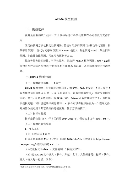
以1996-2005年度各月的全社会用电量作为时间序列,用求和自回归移动平均(ARIMA)乘积模型建模,并且做出1年期的电能消耗预测.将预测结果和2006年1-12月份的实际用电量进行对比,结果比较不错,说明可以用ARIMA模型对县城电力需求做中期预测。
关键词:时间序列;ARIMA模型;预测;SASAbstract: There are some random factors,as well as obvious intrinsic rules,in the counties' year's data of electricity consume. Forecasting counties' electricity demand scientifically is an important basic tasks,and need an forecasting method with easier to use and having sufficient precision.For the purpose of pressing close to practice and easier to checkout,an ARIMA model of time series according to the 1996-2005 electricity consume in Shizhu is proposed.Forecast of one-year's electricity demand is made using this model,and the forecasting results are contrasted with the actual electricity consume during 1-12 months of 2006.The Results show that the method can be applied to medium term's forecasting of counties' electricity demand.Keywords: time series; ARIMA model; forecasting; SAS科学预测县城电力负荷需求,是合理安排扩大发电能力计划的依据,也是有效实施电力需求侧管理的重要手段。
ARIMA模型预测【范本模板】
ARIMA模型预测一、模型选择预测是重要的统计技术,对于领导层进行科学决策具有不可替代的支撑作用.常用的预测方法包括定性预测法、传统时间序列预测(如移动平均预测、指数平滑预测)、现代时间序列预测(如ARIMA模型)、灰色预测(GM)、线性回归预测、非线性曲线预测、马尔可夫预测等方法。
综合考量方法简捷性、科学性原则,我选择ARIMA模型预测、GM(1,1)模型预测两种方法进行预测,并将结果相互比对,权衡取舍,从而选择最佳的预测结果。
二ARIMA模型预测(一)预测软件选择-—--R软件ARIMA模型预测,可实现的软件较多,如SPSS、SAS、Eviews、R等。
使用R 软件建模预测的优点是:第一,R是世最强大、最有前景的软件,已经成为美国的主流。
第二,R是免费软件。
而SPSS、SAS、Eviews正版软件极为昂贵,盗版存在侵权问题,可以引起法律纠纷.第三、R软件可以将程序保存为一个程序文件,略加修改便可用于其它数据的建模预测,便于方法的推广。
(二)指标和数据指标是销售量(x),样本区间是1964-2013年,保存文本文件data。
txt中.(三)预测的具体步骤1、准备工作(1)下载安装R软件目前最新版本是R3。
1.2,发布日期是2014-10—31,下载地址是http://www。
r—/.我使用的是R3。
1.1。
(2)把数据文件data.txt文件复制“我的文档"①。
(3)把data.txt文件读入R软件,并起个名字。
具体操作是:打开R软件,输入(输入每一行后,回车):①我的文档是默认的工作目录,也可以修改自定义工作目录。
data=read.table("data.txt",header=T)data #查看数据①回车表示执行。
完成上面操作后,R窗口会显示:(4)把销售额(x)转化为时间序列格式x=ts(x,start=1964)x结果:2、对x进行平稳性检验ARMA模型的一个前提条件是,要求数列是平稳时间序列。
金融时间序列分析-ARIMA模型建模实验报告
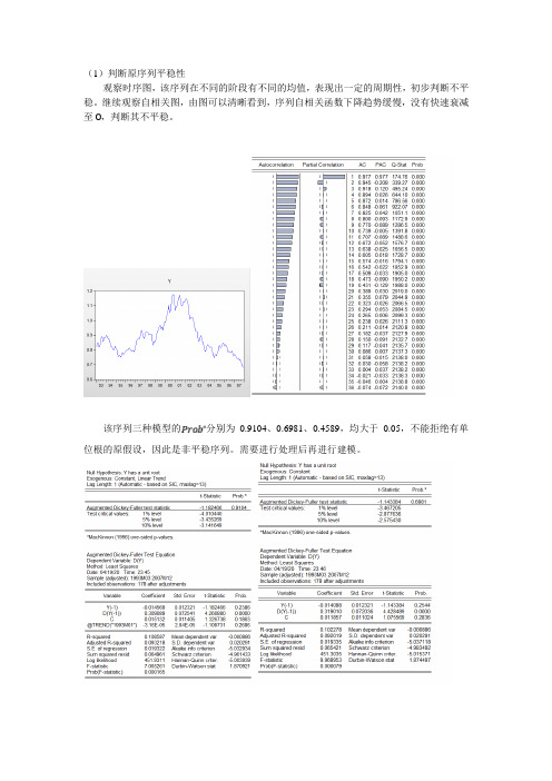
(1)判断原序列平稳性观察时序图,该序列在不同的阶段有不同的均值,表现出一定的周期性,初步判断不平稳。
继续观察自相关图,由图可以清晰看到,序列自相关函数下降趋势缓慢,没有快速衰减至0,判断其不平稳。
该序列三种模型的分别为0.9104、0.6981、0.4589,均大于0.05,不能拒绝有单位根的原假设,因此是非平稳序列。
需要进行处理后再进行建模。
(2)差分序列平稳性检验对原序列进行一次差分,再对其进行平稳性检验。
观察其时序图,该序列的时序图都表现出围绕其水平均值不断波动的过程,没有明显的趋势或周期性,粗略估计是平稳时间序列。
再观察其自相关函数图。
自相关系数快速衰减到0,在虚线范围内波动,没有明显的波动、发散,判断为平稳序列。
模型3与模型2的伴随概率为0,拒绝有单位根的原假设,说明序列是平稳的。
但模型3的时间趋势项的伴随概率为0.1789,常数项的伴随概率0.3504,在显著性水平0.05情况下不显著,故不选用。
而模型2的常数项的伴随概率为0.6608,也不显著,不选用。
因此模型1是最合适的模型,不含有常数项和时间趋势项。
(3)模型的参数估计及模型的诊断检验观察自相关图最后两列可以看到,Q检验的伴随概率均小于0.05,拒绝没有自相关性的原假设,因此该序列不是白噪声序列,没有把信息都提取出来。
接下来将尝试使用AR(1)、AR(2)、AR(3)、MA(1)、ARMA(1,1)、ARMA(2,1)模型进行拟合。
(1)AR(1):该模型各项显著,故对其进行残差项白噪声检验,观察Q检验及其伴随概率,在显著性水平为0.05时,拒绝没有自相关性的原假设,不是白噪声序列,不选用。
(2)AR(2):。
该模型各项显著,故对其进行残差项白噪声检验,观察Q检验及其伴随概率,在显著性水平为0.05时,接受没有自相关性的原假设,是白噪声序列,可以选用。
(3)AR(3):该模型各项不显著,不选用。
(4)MA(1):该模型各项显著,故对其进行残差项白噪声检验,观察Q检验及其伴随概率,在显著性水平为0.05时,接受没有自相关性的原假设,是白噪声序列,可以选用。
时间序列分析与预测:ARIMA模型的应用说明书
Prediction of US Stocks Based on ARIMA ModelBoyu Xiao(B)Guangdong University of Foreign Studies,Guangzhou,China*********************Abstract.Time series analysis method is an important part of statistics.It haspractical applications in variousfields from economics to engineering.Time seriesanalysis includes analyzing time series data in order to extract meaningful featuresof data and predict future values.Box-Jenkins method belongs to regression anal-ysis method and is the basic method of time series analysis and prediction.Thispaper describes the modeling method and implementation process of ARIMA.A time series is a series of data points,usually measured at uniform time inter-vals.Autoregressive integral moving average(ARIMA)model is a kind of linearmodel that can represent stationary and non-stationary time series.ARIMA modeldepends on autocorrelation mode to a large extent.This paper will discuss theapplication in stock price forecasting,especially the time sampling at differenttime intervals,to determine whether there are some optimal design frameworksand whether the stock autocorrelation patterns in the same industry are similar.Keywords:ARIMA·Stock price forecast1IntroductionThe development of the economy has led to the rapid development of the stock market, and the stock market has become another mirror of the national economy,and more and more people choose to invest idle funds in the low-cost,high-return stock market.Stock price prediction is an operation tofind out the law of the stock market,make reasonable trend judgment according to the law,and then guide investment behavior.Therefore, stock price forecasting not only helps the government to carry out macro-control,but also guides investors to make rational choices[1,2].2Modeling and Forecasting of FORECAST2.1Stepwise Autoregressive Models in Time Series AnalysisPROC FORECAST can be used to automatically model and predict AMEX closing prices,Jones Industrial average closing prices,and gold spot prices in New York City as data for step-by-step autoregressive and exponential smoothing models.Before making predictions with PROC FORECAST,the datasets are consolidated and collated.Data set AMEX1,Data set GOLD,Dataset DJsections are shown in Table 1[3].Table2and Table3show the output of a stepwise autoregressive model.©The Author(s)2023Y.Jiang et al.(Eds.):ICFIED2023,AEBMR237,pp.312–322,2023.https:///10.2991/978-94-6463-142-5_35Prediction of US Stocks Based on ARIMA Model313Table1.Data set AMEX1,GOLD and DJAMEX1day AMEX1close DJday DJclose GOLDday GOLDclose 102AUG93437.8803JAN941144.88O3JAH94393.7203AUG93437.2904JAN941123.69O4JAK94394.1304AIK93436,4205JAN941120.6605JAH94391.1405AUG93435.5306JAN941133.1606JAH94389.2506AUG93436.3407JWI941138.7607JAH94386.4609AUG93438.8010JAN941169.9110JAU94385710AUG93439.19343451171.74UJAK943888UAUG93438.87343461153.2912JAK94386.3912AUG93437.5813JAN941145.8913JMJ9439010I3AUG93439.0814JAN941149.78I4JA1R4389.5Table2.The output of a stepwise autoregressive model(1) type day close closing price CGMEX gold Spot Closing Pricefor Day1N25MAR945959592WRESID25MAR945959593DF25MAR945656564SIGhlA25MAR9412.43386 2.2308667316620045CONSTANT25MAR941122.4786484.24895386.855016LINEAR25MAR940.8647664-0.284715-0.0881527ARI25MAR940.8804790.8468460.75482118AR225MAK949AR325MAR9410AR425MAR94Table3.The output of a stepwise autoregressive model(2) day type dj_close closing price CGMEX gold Spot ClosingPrice for Day128MAR94FORECAST1190.8802343467.9517099388.6987963229MAR94FORECAST1189.8743949467.5030667386.7647041330HAR94FORECAST1189.0921321467.7952977385.3586797(continued)314 B.XiaoTable3.(continued)day type dj_close closing price CGMEX gold Spot ClosingPrice for Day431KAR94FORECAST1188.5067238466.6772541384.2757695501APR94FORECAST1188.0946419466.2929833383.4367631604APR94FORECAST1187.8361702466.9239600382.7818327705APR94FORECAST1187.7100685465.5678488382.2658719806APR94FORECAST1187.7032769465.2226724381.8548007907APR94FORECAST1187.8006547464.8867559381.52290241008APR94FORECAST1187.9897516464.5586812381.2507655Table4.Exponential smoothing model datatype day dj_close closing price COMEX gold Spot Closing Pricefor Day1N25-Mar-945959592KRISID25-Mar-945959593DF25-Mar-945656564WEIGHT25-Mar-940.2020.25SI25-Mar-941191458247010675387676966S225-Mar-9411800942469.71516384936887S325-Mar-941169.099646939076382932438SICMA25-Mar-941790133826944957387994299COKSTAITT25-Mar-941203.1918047056553911526710LIBEAR25-Mar-94 3.03729820133581910758252………………2.2Exponential Smoothing Model in Time Series Analysis(as Table4)2.3Empirical and Comparative of Stepwise Autoregressive Modelsand Exponential Smoothing ModelsFor any time series,you must choose the model that best reflects the trend of the data, and the goodness-of-fit statistic is a common criterion for selecting models.Table5 compares the variable CLOSE using a stepwise autoregressive model and an exponential smoothing model goodness-of-fit statistics.It can be observed from the table that in the statistics(SSE,MSE,PMSE,MAPE, MPE,MAE,ME),the values corresponding to the stepwise autoregressive model are all smaller than the exponential smoothing model,such as SSE293.28,which is smaller thanPrediction of US Stocks Based on ARIMA Model315 Table5.Stepwise autoregressive models and exponential smoothing models goodness-of-fit comparison tableExtrapolate the time series model AMEX index closing priceStatistics AMEX Index Closing Price ModelGradual self-regression Exponential smoothingSSE293.28332376.95883MSE 5.2372021 6.7314077RMSE 2.2884934 2.5944957MAPE0.34649970.3906927MPE0.00019610.0467643MAE 1.6465708 1.8553361ME0.01081270.22273171RSQUARE0.87987780.8456062ADJRSQ0.87558770.8400922RW_RSQ-0.04846-0.347592ARSQ0.86700760.829064APC 5.50355057.0736827AIC100.6125115.42131SBC106.84511121.65393SSE376.96;in addition,The value of the stepwise autoregressive model is closer to1than the exponential smoothing model,for example,RSQUARE(stepwise autoregressive model)0.88is greater than RSQUARE(exponential smoothing model)0.85.This shows that the stepwise autoregressive modelfits the past values of the AMEX index closing price series better.2.4Forecasting for Extrapolated Time Series ModelsFrom this,the model predictions of the stepwise autoregressive and exponential smoothing models are obtained(as Fig.1and Fig.2).Interpretation of the results:The predictions of the autoregressive model and the exponential smoothing model predict different expectations.The autoregressive model predicts an uptrend for the DJIA and a downtrend for the AMEX index closing price and gold spot price,while the exponential smoothing model predicts an uptrend for the DJIA and an uptrend for the AMEX index and gold.316 B.XiaoFig.1.Forecast Stepwise Autoregressive ModelFig.2.Exponential Smoothing Model Prediction3Build Models with PROC ARIMA3.1Build and Compare Time Series Analysis Models by PROC ARIMAThe ARIMA model has three parameters(p,d,q),where p refers to the order of the autoregressive part of the model,d refers to the number of sequence differences,and q refers to the number of average moving parts of the model.The AMEX index closing price series is shown in Fig.3.After thefirst differencing,the sequence exhibits stability. After selecting an appropriate model,the sequence can be predicted[4,5].Through the analysis of the above results,the following conclusions are drawn: (1)Parameter estimates,approximate standard errors,t-ratios,and lags for the specifiedmodel.The only parameters estimated are the mean(MU or constant)with a value of-0.15316,an approximate standard error of0.44596and a t-ratio of-0.34. (2)The constant estimate represents the intercept parameter of the MA model adjustedfor all AR parameters.If the AR parameter is not included in the model,the constantPrediction of US Stocks Based on ARIMA Model 317Fig.3.A Stochastic Model of the First Difference of AMEX Index Closing PricesTable 6.Model Comparison ResultsModel Statistics Stochastic Models with Trends (0,1,0)random walk (1,1,0)AR (1)(1,1,0)MA (1)(0,1,1)ARIMA (1,1,1)Parameter EstimationMU-0.15316(-0.34)N/AMU-0.16306(-0.33)MU-0.16186(-0.32)MU-0.11633(-0.24)AR10.07326(0.30)MA1-0.09860(-0.41)MA1-0.96017(-5.46)AR1-0.81492(-2.82)variance 3.763501 3.588879 3.963963 3.95612 3.993331AIC 80.0740378.1986281.9740281.9363982.9624SBC 81.0184778.1986283.862983.8252785,79572Q lag6123(0.9754) 1.38(0.9669)117(0.9479)0.76(0.9439)Iagl2 4.16(0.9804) 4.26(0.9783)411(0.9665) 2.96(0.9823)Iagl813.06(0.7880)14.52:(0.6945)12.19(0.7887)10.51(0.8386)estimate and the mean parameter estimate are identical.If the model contains an AR(p)component,the constant in the output is estimated as.(3)The goodness-of-fit statistics are variance,standard deviation,Akaike InformationCriterion (AIC)and Schwartz-Bayesian Criterion (SBC).The better the estimated model fits,the smaller these statistics will be.(4)A list of test statistics (i.e.chi-square or Q-statistics)for the white noise hypothesisof the fitted model residuals.The null hypothesis is that the residuals are white noise.The p-value indicates that the null hypothesis cannot be rejected at the 0.05significance level.The above table only outputs random models,and Table 6lists the results for these models for ease of comparison [6].Overall,the random walk (0,1,0)model and the ARIMA (1,1,1)model are better than other models,so they are used as alternative models for the next comparison.318 B.XiaoFig.4.Different models of AMEX index closing prices correspond to forecast values3.2Comparing the Random Walk(0,1,0)Model and the ARIMA(1,1,1)Model 3.2.1Forecasting Using PROC ARIMAYou can use PROC ARIMA to predict the future value of the time series,use the ARIMA (0,1,0)model and ARIMA(1,1,1)model with a certain trend to predict the future value of the AMEX index closing price,and output the predicted value(as Fig.4)[7,8].The table above outputs the actual and predicted values,standard errors,95%upper and lower confidence limits,and residuals for the two models,whose point estimates differ only slightly.The predicted value of the random walk model on March28,1994 is468.43,while the predicted value of the ARIMA(1,1,1)model is slightly lower than the former.The prediction confidence interval(upper bound minus lower bound)of the random walk model(0,1,0)is smaller than that of the ARIMA(1,1,1)model.This is because ARIMA(0,1,0)has fewer parameters to estimate and the standard error STD is small,so if the predictions are very similar,the ARIMA(0,1,0)random walk model should be chosen.3.2.2AMEX Prediction with PROC ARIMAThe examples in this section examine the closing prices of the AMEX index in early 1994.A time series modelfits the series.Through thefigure below,it is believed that the sequence may show a certain trend during the period from February28to March25.As can be seen from the chart below,the sequence reached473.38points on March 23rd,then fell to469.66points on the24th,and extended to468.43points on the25th. The series of predicted values for the random walk model in the table below will remain at468.43in the short term.A very important question is whether the series reached a turning point on March23rd that created a new trend,or whether the apparent dip from March23rd to25th was just randomfluctuations.If the previous trend was still valid,the series would be expected to follow the predicted values in the graph below,but still between the upper and lower confidence limits.The rule of thumb for technical analysis is that a sequence is valid until there is sufficient evidence that a new trend will be established[9,10].Prediction of US Stocks Based on ARIMA Model319Fig.5.AMEX index closing price forecast(1)3.395%Confidence Interval Plot for Random(0,1,0)ModelThe following three graphs generated by PROC GPLOT show the predicted xvalue of the series and the upper and lower confidence limits of the predicted value day by day (as Fig.5,Fig.6and Fig.7).Thefirst graph is from March26,and the second graph is added to the AMEX closing price on March30.Technical analysis charts usually have multiple interpretations.Before using PROC GPLOT,merge the data sets through the DATA step and delete unnecessary values.PROC SORT is used to ensure that these observations are plotted in the proper order.3.495%Confidence Interval Plot for a Stochastic(0,1,0)Model with AddedInformationAdd to the actual closing data on March30,1994.3.595%Confidence Interval Plotting for the Random(0,1,0)Model for MoreInformationAdding to the actual closing data for April11,1994.In a time series analysis model,if the trend is still valid,the series will be carried forward with predicted values and confidence limits.The above chart shows that the actual closing price on the28th was lower than the predicted value and lower than the lower confidence limit.This observation is a strong indication that the sequence has changed.The chart above shows that the actual closing prices on the29th,30th and31st continued to fall and were well below the lower confidence limit.320 B.XiaoFig.6.AMEX index closing price forecast(2)Fig.7.AMEX index closing price forecast(3)4Tests for AMEX Predicted ValuesThe above model can be used to predict the AMEX index closing price(CLOSE).This example uses the second intervention model to predict the value of the CLOSE variable on March29and March30.Figure8is the predicted value of the random walk model(0,1,0)without using the intervention model before.The actual values,predicted values,95%confidence intervals,and known residuals are listed above for March29.In the above table,using the information on March25,the stochastic model wasfitted to obtain the closing price of the AMEX index for the weekPrediction of US Stocks Based on ARIMA Model321Fig.8.AMEX index closing price forecast based on stochastic(0,1,0)model without intercept termof March28to be468.43;the actual values of March28and29were462.21and454.43, Then the predicted value of the random walk model for March30and31(468.43)is questionable.Because the intervention model forecast includes two other actual series values and takes advantage of the downtrend from March23rd,it should be more precise [6,11].5ConclusionTo sum up,the intervention model is relatively accurate relative to the random walk model(0,1,0)and the ARIMA model,but there is also a certain prediction bias.When you are satisfied with the analysis and forecast of the series,the next practical operation is to sell stocks that continue to decline and buy and hold stocks that are going to rise. When buying and selling stocks,you can control the situation through the choice of buying stocks,buy stocks that are forecast to rise at any time,and sell stocks that are forecast to fall,so as to reap benefits in the ups and downs.References1.Burges C.A Tutorial on Support Vector Machines for Pattern Recognition[J].Data Miningand Knowledge Discovery,1998,2.2.Wang Xiaopeng,Cao Guangchao,Ding Shengxi.Analysis,modeling and prediction of pre-cipitation time series on the Qingnan Plateau based on Box-Jenkins method[J].Mathematical Statistics and Management,2008(04):565-570.DOI:https:///10.13860/ki.sltj.2008.04.001.3.Chi Qishui.Analysis on the growth trend of China’s oil consumption——Prediction andanalysis based on ARIMA model[J].Resource Science,2007(05):69–73.4.Bai Yingshan.Prediction and Analysis of CSI300Index Based on ARIMA Model[D].SouthChina University of Technology,2010.5.Ding parison of ARIMA Model and LSTM Model Based on Stock Predic-tion[J].Industrial Control Computer,2021,34(07):109–112+116.322 B.Xiao6.Hou Lu.Short-term analysis and forecast of oil price based on ARIMA model[D].JinanUniversity,2009.7.Gong Guoyong.Application of ARIMA Model in Shenzhen GDP Forecast[J].Practice andUnderstanding of Mathematics,2008(04):53-57.8.Hua Peng,Zhao Xuemin.Application of ARIMA Model in GDP Forecasting of Guang-dong Province[J].Statistics and Decision-Making,2010(12):166-167.DOI:https:///10.13546/ki.tjyjc.2010.12.016.9.Li Shengbiao.Analysis and prediction of commodity housing prices in Lanzhou City basedon ARIMA model[J].Gansu Science and Technology,2014,30(21):93–94+66.10.Xu Liping,Luo Mingzhi.Short-term analysis and forecast of gold price based on ARIMAmodel[J].Finance and Economics,2011(01):26-34.11.Wu Yuxia,Wen Xin.Short-term stock price forecast based on ARIMA model[J].Statistics andDecision-Making,2016(23):83-86.DOI:https:///10.13546/ki.tjyjc.2016.23.051. Open Access This chapter is licensed under the terms of the Creative Commons Attribution-NonCommercial 4.0International License(/licenses/by-nc/4.0/), which permits any noncommercial use,sharing,adaptation,distribution and reproduction in any medium or format,as long as you give appropriate credit to the original author(s)and the source, provide a link to the Creative Commons license and indicate if changes were made.The images or other third party material in this chapter are included in the chapter’s Creative Commons license,unless indicated otherwise in a credit line to the material.If material is not included in the chapter’s Creative Commons license and your intended use is not permitted by statutory regulation or exceeds the permitted use,you will need to obtain permission directly from the copyright holder.。
- 1、下载文档前请自行甄别文档内容的完整性,平台不提供额外的编辑、内容补充、找答案等附加服务。
- 2、"仅部分预览"的文档,不可在线预览部分如存在完整性等问题,可反馈申请退款(可完整预览的文档不适用该条件!)。
- 3、如文档侵犯您的权益,请联系客服反馈,我们会尽快为您处理(人工客服工作时间:9:00-18:30)。
实验指导书(ARIMA模型建模与预测)例:我国1952-2011年的进出口总额数据建模及预测1、模型识别和定阶(1)数据录入打开Eviews软件,选择“File”菜单中的“New--Workfile”选项,在“Workfile structure type”栏选择“Dated –regular frequency”,在“Date specification”栏中分别选择“Annual”(年数据) ,分别在起始年输入1952,终止年输入2011,文件名输入“im_ex”,点击ok,见下图,这样就建立了一个工作文件。
在workfile中新建序列im_ex,并录入数据(点击File/Import/Read Text-Lotus-Excel…,找到相应的Excel数据集,打开数据集,出现如下图的窗口,在“Data order”选项中选择“By observation-series in columns”即按照观察值顺序录入,第一个数据是从B15开始的,所以在“Upper-left data cell”中输入B15,本例只有一列数据,在“Names for series or number if named in file”中输入序列的名字im_ex,点击ok,则录入了数据):(2)时序图判断平稳性双击序列im_ex,点击view/Graph/line,得到下列对话框:显著非平稳。
IM_EX240,000200,000160,000120,00080,00040,000556065707580859095000510(3因为数据有指数上升趋势,为了减小波动,对其对数化,在Eviews命令框中输入相应的命令“series y=log(im_ex)”就得到对数序列,其时序图见下图,对数化后的序列远没有原始序列波动剧烈:45678910111213556065707580859095000510Y从图上仍然直观看出序列不平稳,进一步考察序列y 的自相关图和偏自相关图:从自相关系数可以看出,呈周期衰减到零的速度非常缓慢,所以断定y 序列非平稳。
为了证实这个结论,进一步对其做ADF 检验。
双击序列y ,点击view/unit root test ,出现下图的对话框,我们对序列y 本身进行检验,所以选择“Level ”;序列y 存在明显的线性趋势,所以选择对带常数项和线性趋势项的模型进行检验,其他采用默认设置,点击ok 。
检验结果见下图,可以看出在显著性水平0.05下,接受存在一个单位根的原假设,进一步验证了原序列不平稳。
为了找出其非平稳的阶数,需要对其一阶差分序列和二阶差分序列等进行ADF 检验。
(4)差分次数d 的确定y 序列显著非平稳,现对其一阶差分序列进行ADF 检验。
在对y 的一阶差分序列进行ADF 单位根检验之前,需要明确y 的一阶差分序列的趋势特征。
在Eviews 命令框中输入相应的命令“-.4-.2.0.2.4.6556065707580859095000510DY1由y 因此,在下图对序列y 的单位根检验的对话框中选择“1st difference ”,同时选择带常数项、不带趋势项的模型进行检验,其他采用默认设置,点击ok 。
检验结果见下图,可以看出在显著性水平0.05下,拒绝存在单位根的原假设,说明序列y 的一阶差分序列是平稳序列,因此d=1。
(5)建立一阶差分序列在Eviews 对话框中输入“series x=y-y(-1)”或“series x=y-y(-1)”,并点击“回车”,便得到了经过一阶差分处理后的新序列x ,其时序图见下图,从直观上来看,序列x 也是平稳的,这就可以对x -.4-.2.0.2.4.6556065707580859095000510X(6双击序列x ,点击view/Correlogram ,出现下图对话框,我们对原始数据序列做相关图,因此在“Correlogram of ”对话框中选择“Level ”即表示对原始序列做相关,在滞后阶数中选择12(或8=60⎡⎤⎣⎦),点击ok ,即出现下列相关图:从x 的自相关函数图和偏自相关函数图中我们可以看到,偏自相关系数是明显截尾的,而自相关系数在滞后6阶和7阶的时候落在2倍标准差的边缘。
这使得我们难以采用传统的Box-Jenkins 方法(自相关偏自相关函数、残差方差图、F 检验、准则函数)确定模型的阶数。
对于这种情况,本例通过反复对模型进行估计比较不同模型的变量对应参数的显著性来确定模型阶数。
2、模型的参数估计在Eviews 主菜单点击“Quick ”-“Estimate Equation ”,会弹出如下图所示的窗口,在“Equation Specification ”空白栏中键入“x C AR(1) AR(2) MA(1) MA(2) MA(3) MA(4) MA(5)”等,在“Estimation Settings ”中选择“LS-Least Squares(NLS and ARMA)”,然后“OK ”。
或者在命令窗口直接输入“ls x C AR(1) AR(2) MA(1) MA(2) MA(3) MA(4) MA(5)”等。
针对序列x 我们尝试几种不同的模型拟合,比如ARMA(1,7),ARMA(1,6),ARMA(2,6)等。
各种模型的参数显著性t 检验的结果(p 值)见下表(不显著为零的参数的p 值用红色字体表示)可见,各种估计模型的参数显著性检验中,只有黄色覆盖的包含部分参数的三个模型ARMA(2,7)、ARMA(1,7)和ARMA(1,6)所有参数都显著,现在来比较上述模型的残差方差和信息准则值由上表可见,方程Eq02_07_2对应的ARMA(2,7)模型的残差方差最小,其次是方程Eq01_06_1对应的ARMA(1,6)模型的残差方差;而方程Eq01_06_1对应的ARMA(1,6)模型的AIC 和BIC 信息准则都小于方程Eq02_07_2对应的ARMA(2,7)模型的AIC 和BIC 信息准则,且在估计的模型中,方程Eq01_06_1对应的ARMA(1,6)模型的AIC 和BIC 信息准则最小,而且由各个模型系数的t 检验统计量的p 值可知,在方程Eq01_06_1对应的ARMA(1,6)模型中所有模型的系数都显著不为零。
所以,我们这里选择由方程Eq01_06_1对应的ARMA(1,6)模型。
该模型的估计结果如下由结果可见,模型的最小二乘估计结果为1126ˆ0.1516760.7854400.4633910.4283910.454978(3.179728)(9.965828)( 4.109880)( 3.726979)(11.13043)t t t t t X X a a a ----=+--+--误差项方差的估计值为ˆ0.138901a σ= 并且由模型的系数的t 统计量及其p 值也可以看到,模型所有解释变量的参数估计值在0.01的显著性水平下都是显著的。
3、模型的适应性检验参数估计后,应对拟合模型的适应性进行检验,实质是对模型残差序列进行白噪声检验。
若残差序列不是白噪声,说明还有一些重要信息没被提取,应重新设定模型。
可以对残差进行纯随机性检验,也可用针对残差的2χ检验。
(1) 残差序列的生成残差序列从1954至2011年采用拟合的ARMA(1,6)模型生成,在方程窗口点击proc/make residual series …,得到下列对话框将该方程的残差序列定义为a_eq01_06_1即可,可以得到从1954至2011年采用拟合的ARMA(1,6)模型生成的残差序列。
前面的1953则是将前面的初始值012012,,,;,,,X X X a a a ----L L 都设为0而计算的。
程序命令如下a_eq 01_06_1 (2)=x(2)-0.151676-0.785440*0+0.463391*0+0.428391*0-0.454978*0这样得到的序列a_eq01_06_1即为ARMA(1,6)模型的残差序列,a_eq01_06_1序列的自相关偏自相关图如下:(偏)相关函数值、以及Q-Stat 及其p 值显示,残差序列不存在自相关,为白噪声,因此模型是适合的模型。
模型拟合图如下-.4-.2.0.2.4-.4-.2.0.2.4.6556065707580859095000510Residual Actual Fitted(8)模型预测我们用拟合的有效模型进行短期预测,比如我们预测2012年、2013年、2014年和2015年的进出口总额。
先预测2012年、2013年、2014年和2015年的x,再预测进出口总额。
首先需要扩展样本期,在命令栏输入expand 1952 2015,回车则样本序列长度就变成64了,且最后面4个变量值为空。
在方程估计窗口点击Forecast,出现下图对话框,预测方法常用有两种:Dynamic forecast和Static forecast:动态预测是根据所选择的一定的估计区间,进行多步向前预测(从预测样本的第一期开始计算多步预测):dynamic dynamic dynamic11dynamic dynamic26ˆˆˆ0.1516760.7854400.463391ˆˆ0.4283910.4549782012,2013,21954,1955,014,2015,2011,t t tt tX X aa at----=+--+=L每一步都是采用前面的预测值计算新的预测值。
而样本范围内(1954-2011)的序列实际值是已知的。
因此,动态预测只是适应于样本外(2012-2015)预测,而不适应于样本内(1954-2011)预测。
静态预测是滚动的进行向前一步预测,即每预测一次,用真实值代替预测值,加入到估计区间,再进行向前一步预测(利用滞后因变量的实际值而不是预测值计算一步向前(one-step-ahead )预测的结果):static 1126ˆ0.1516760.7854400.4633910.4283910.4549781954,1955,,2012012,1,t t t t t X X a a a t ----=+--+=L L可见,对于样本外(2012-2015)的预测需要提供样本外预测期间的解释变量值。
对静态预测,还必须提供滞后因变量的数值。
而对于样本外(2012-2015)的预测通常因变量的实际观测值是未知的,所以,静态预测一般只适应于样本内(19542011)预测,不适应于样本外预测(只可以进行向前一步样本外预测)。
并且,由计算公式可见,样本内(1954-2011)的静态预测值与模型的拟合值(估计值)相同。