Simulating the Quantum Fourier Transform with Distributed Computing
量子纠缠的数学原理

量子纠缠的数学原理Quantum entanglement is one of the most fascinating phenomena in quantum mechanics. It refers to the strong correlation that exists between particles even when they are separated by large distances. This phenomenon was famously described by Albert Einstein as "spooky action at a distance," highlighting its counterintuitive nature.量子纠缠是量子力学中最令人着迷的现象之一。
它指的是即使粒子相距很远,它们之间仍存在强烈的相关性。
爱因斯坦曾将这一现象形象地描述为“鬼魅般的遥远作用”,突显其反直觉的本质。
One of the key mathematical principles that underpin quantum entanglement is superposition. In simple terms, superposition allows a quantum system to exist in multiple states simultaneously until it is measured or observed. This property is crucial for understandinghow entangled particles can be in a state of flux, with their properties being intrinsically linked regardless of the distance between them.支撑量子纠缠的关键数学原理之一是叠加原理。
Quantum CPU and Quantum Algorithm
IA , thus cA and c† A can be thought of as the fermionic annihilate and create operators respectively in the auxiliary qubit. In order to give out the realization of QCPU for the product of transformation in a form of full multiplication, eq.(3) can be rewritten as
2k −1
Q(U ) =
m,n=0
† exp{(Umn |m n| ⊗ IA ) · CA }
(1)
where IR and IA are the identity matrices in the register space and the auxiliary qubit space
† respectively, and CA = IR ⊗ c† A = IR ⊗ |1 AA
Quantum computing [1,2] has attracted a lot of physicists since Shor found his quantum algorithm of factorization of a large number. [3] This is because that Shor’s algorithm can speed up exponentially the factorization computation in a quantum computer than doing this in a classical computer. From then, quantum computer appears very promising and quantum algorithm plays a vital role. Actually, the high efficiency of quantum computer is just profited by the good quantum algorithms. Both classical and quantum algorithms consist of a series of quantum computing steps. In the quantum algorithm, a computing step can be a transformation or a quantum measurement. The final quantum computing task made of these steps is represented usually by the summation and product of them, which formed an total unitary transformation. In order to implement a given quantum algorithm including quantum simulating procedure, one needs to design, assemble and scale these quantum computing steps so that one finally
2Wave-optics simulation of the channel fading in modulating retro-reflector free-space optical link
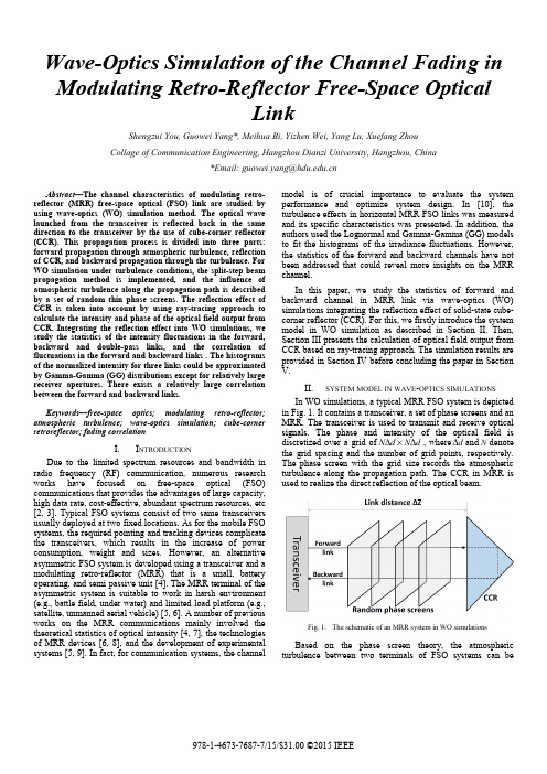
Wave-Optics Simulation of the Channel Fading in Modulating Retro-Reflector Free-Space OpticalLinkShengzui You, Guowei Yang*, Meihua Bi, Yizhen Wei, Yang Lu, Xuefang ZhouCollage of Communication Engineering, Hangzhou Dianzi University, Hangzhou, China*Email: guowei.yang@Abstract—The channel characteristics of modulating retro-reflector (MRR) free-space optical (FSO) link are studied by using wave-optics (WO) simulation method. The optical wave launched from the transceiver is reflected back in the same direction to the transceiver by the use of cube-corner reflector (CCR). This propagation process is divided into three parts: forward propagation through atmospheric turbulence, reflection of CCR, and backward propagation through the turbulence. For WO simulation under turbulence conditions, the split-step beam propagation method is implemented, and the influence of atmospheric turbulence along the propagation path is described by a set of random thin phase screens. The reflection effect of CCR is taken into account by using ray-tracing approach to calculate the intensity and phase of the optical field output from CCR. Integrating the reflection effect into WO simulations, we study the statistics of the intensity fluctuations in the forward, backward and double-pass links, and the correlation of fluctuations in the forward and backward links . The histograms of the normalized intensity for three links could be approximated by Gamma-Gamma (GG) distributions except for relatively large receiver apertures. There exists a relatively large correlation between the forward and backward links.Keywords—free-space optics; modulating retro-reflector; atmospheric turbulence; wave-optics simulation; cube-corner retroreflector; fading correlationI.I NTRODUCTIONDue to the limited spectrum resources and bandwidth in radio frequency (RF) communication, numerous research works have focused on free-space optical (FSO) communications that provides the advantages of large capacity, high data rate, cost-effective, abundant spectrum resources, etc [2, 3]. Typical FSO systems consist of two same transceivers usually deployed at two fixed locations. As for the mobile FSO systems, the required pointing and tracking devices complicate the transceivers, which results in the increase of power consumption, weight and sizes. However, an alternative asymmetric FSO system is developed using a transceiver and a modulating retro-reflector (MRR) that is a small, battery operating, and semi passive unit [4]. The MRR terminal of the asymmetric system is suitable to work in harsh environment (e.g., battle field, under water) and limited load platform (e.g., satellite, unmanned aerial vehicle) [5, 6]. A number of previous works on the MRR communications mainly involved the theoretical statistics of optical intensity [4, 7], the technologies of MRR devices [6, 8], and the development of experimental systems [5, 9]. In fact, for communication systems, the channel model is of crucial importance to evaluate the system performance and optimize system design. In [10], the turbulence effects in horizontal MRR FSO links was measured and its specific characteristics was presented. In addition, the authors used the Lognormal and Gamma-Gamma (GG) models to fit the histograms of the irradiance fluctuations. However, the statistics of the forward and backward channels have not been addressed that could reveal more insights on the MRR channel.In this paper, we study the statistics of forward and backward channel in MRR link via wave-optics (WO) simulations integrating the reflection effect of solid-state cube-corner reflector (CCR). For this, we firstly introduce the system model in WO simulation as described in Section II. Then, Section III presents the calculation of optical field output from CCR based on ray-tracing approach. The simulation results are provided in Section IV before concluding the paper in Section V.II.SYSTEM MODEL IN WAVE-OPTICS SIMULATIONSIn WO simulations, a typical MRR FSO system is depicted in Fig. 1. It contains a transceiver, a set of phase screens and an MRR. The transceiver is used to transmit and receive optical signals. The phase and intensity of the optical field is discretized over a grid of dNdNΔ×Δ, where dΔand N denote the grid spacing and the number of grid points, respectively. The phase screen with the grid size records the atmospheric turbulence along the propagation path. The CCR in MRR is used to realize the direct reflection of the optical beam.Fig. 1.The schematic of an MRR system in WO simulations Based on the phase screen theory, the atmosphericturbulence between two terminals of FSO systems can be 978-1-4673-7687-7/15/$31.00 ©2015 IEEEapproximated by a series of random phase screens [11, 12]. To generate the random phase screens, the most common way is that taking inverse Fourier transform of atmospheric refractive-index power spectral density (PSD) [13, 14]. Accordingly, the irradiance variance on the observation plane (i.e., receiver plane) can be obtained byi i nni z z z C z k Δ⎟⎠⎞⎜⎝⎛Δ−Δ=∑6512656721563.0σ.(1)Where 2ni C is the refractive index structure parameter. λπ2=k is the wavenumber. z Δis the link distance. i z is the distance from the transceiver to the i -th phase screen. i z Δis propagation distance from the i -th to (i+1)-th plane. n represents the number of total phase screens.To simulate the optical beam propagation from the i -th screen to (i+1)-th screen, the well-knowm split-step beam propagation method is used. Let us denote by )(i r S the optical field on the i -th screen, and i r denotes the coordinate on the i -th screen. ()()11exp ],[++−=i i i r i z z T φ denotes an operator that represents the phase accumulation between the i -th and (i+1)-th screen. The accumulated phase is calculated by()()∫+=1i iz z i i dz r n kr δφ, where )(i r δn represents the refractivefluctuations. According to the split-step beam propagation method, the field )(1+i r S on the (i+1)-th phase screen is calculated by(){}i i i i i i i i i i r S r r z R z z T r r zR r S ]~,,2[],[],~,2[)(11111+++++Δ×Δ≅. (2)Where the Fresnel diffraction operator is(){}()121212121],,[dr er S di r S r r d R r r d k ii −+∞∞−∫=.(3)1~+i r is a coordinate in a plane half-way between the i -th and(i+1)-th screen. Applying the above algorithm recursively from the source screen to the observation screen, we could imitate the optical beam propagating through the atmospheric turbulence from one terminal to another terminal of FSO systems.III. CALCULATION OF OPTICAL FIELD OUTPUT FROM CCRThe CCR consists of three mutually perpendicular,intersecting flat reflective surfaces, as shown in Fig. 2. Notethat we consider the CCR with the circular aperture. The incident light is reflected successively by three surfaces of the CCR, and returned in the opposite direction [15, 16]. In fact,there exists six different reflection orders, i.e., I →II →III ,I →III →II, III →I →II, III →II →I, II →III →I, II →I →III. The sixreflection sequences correspond to six sectorial domains thatmake up the whole effective reflection area of CCR, see Fig. 3.Fig. 2. Light reflected three times in the CCRFig. 3. Six fan-shaped reflection area of CCRTo facilitate the computation, we establish XYZ O - coordinate system for the CCR and optical beam inside, and xyz o - coordinate system for the optical beam outside the CCR. The two coordinate systems are related through a transformation matrix that is given by [16]⎥⎥⎥⎥⎥⎥⎥⎦⎤⎢⎢⎢⎢⎢⎢⎢⎣⎡−−=336622-33360336622M . (4)We consider the incident optical beam with the incident angel ϕand the azimuth angle θ, the unit vector of the incident beam is expressed in xyz o - system as[]T in cos ,sin sin ,cos sin ϕθϕθϕ=′R , (5) where the superscript T denotes the transpose. When the threesides of CCR is completely vertical, it can achieve reversereflection, i.e., the reflected beam vector is illustrate ray-tracing for the CCR, we take order of II →I →III. From Fig. 2, the incidenthe CCR aperture at the point (111,,z y x ′′=′P calculation is carried out in XYZ O -coordin in in R M R ′= and []113,3,3a a a +′=P M P length of CCR aperture side. Using the law vector notation [17], the vector of the refract 1P and 2P can be obtained byN R R p n n +=′in 2CCR1,and()2in 22N R N n n n p −•+−′=where n ′and n represent the refractive ind and refractive medium. [3-,33-=N normal vector of the CCR aperture. For sim []T 321CCR12,,r r r =R and ()1111,,Z Y X =P .()2222,,Z Y X =P is determined by⎪⎩⎪⎨⎧−=−=−=32211211220r Z r Y Y r X X Y Also, the beam vector from 2P and 3P is o(II II 12CCR 23CCR 2N N R R n n •−′=′where II N is the normal vector of the surfac and (9), we could successively obtain the p 5P , and the corresponding beam vectors Also, using (6) and (7), we get the vector system and the corresponding out R ′ in x o -that the calculation should be executed indiv reflection sequences. Also, the coordinates of the beam and the reflection surface shou zero, and should be within the scope of CC satisfying these conditions, the optical rays ar IV.NUMERICAL RESULTIn simulation environments, we cons Gaussian beam at =λ 1.55 um with the beam cm and curvature radius of the phase fro corresponding to a beam divergence of 0.46 pass distance is set to 1km, and the refracti constant =2n C 6.5×10⁻¹⁴ m -2/3 with the inner and the outer scale of turbulence =0L 1.3 m perfect glass CCR with a circular aperture o and the incident light beam is perpendic aperture. Several different receiver aperture i.e., =R D 5, 10, 15, 25, 35, 45, 50, 55, 65 m phase screens is set to 20. The sample numb in out R R ′−=′. To an example in thent beam intersects )1′. The following nate system. Thus,T, where a is thew of refraction in tion beam between (6)in R n •,(7)ex of the incident ]T33-,3is the mplicity, we denote. Then, the point 1Z . (8)obtained by [17])12CCR R n ′,(9)ce II. Based on (8)points 3P ,4P and 34CCR R , 54CCR R . out R in XYZ O -xyzsystem. Note vidually for the six of the intersection uld be greater than CR surfaces. Only re effective [16].Ssider a divergent m waist =0W 1.59 ont =0F -69.9 m, mrad. The single-ive index structurescale =0l 6.1 mmm. We consider aof =CCR D 50 mm, cular to the CCR es are considered, mm. The number of ber and spacing inthe grids are set to =N 512modified von Kármán PSD screens which includes the ef Note that to guarantee enou samples for each channel corresponding histogram.(a)(c) Fig. 4. The intensity distributions (a)incident on the CCR plane, (c) re the re To illustrate one simula distributions transmitted from t CCR plane, reflected from C receiver plane are shown in Fi plane and the receiver plane ar The turbulence effect in the for (a) and (b). The reflection effe (b) and (c) is that the optical in the perfect CCR and that reflec symmetry about the origin. T backward link correspond to Fi In addition, the statisticalbackward transmission links a performance of MRR system been well addressed. We st calculating the histograms of r based on WO simulations. M histograms by Gamma-Gamm widely accepted to model sin histograms of normalized rece GG profiles for the forward lin pass links are plotted in Fig. cases of receiver diameters D Note that the forward links in b 2 and =Δ=Δy x 1 mm. The is used to generate the phase ffect of inner and outer scales. ugh accuracy, at least 4104× were used to calculate the(b)(d)) transmitted from the source plane, (b)eflected from CCR plane, (d) irradiate oneceiver planeation realization, the intensitythe source plane, incident on the CR plane and irradiate on the ig. 4. (Note that here the source re placed in the same position.) ward link is illustrated in Figs. 4 ect of the CCR shown in Figs. 4 ntensity distribution incident on cted from the CCR are rotational The intensity fluctuations in the gs. 4 (c) and (d).l fading models of forward and are important for evaluating the m. However, this issue has not tudy the channel statistics by received intensity for both links Moreover, we fit the obtained ma distribution that has been ngle-pass FSO links [11]. The eived intensity and the best-fit nks, backward links and double-5 and 6 corresponding to the =R 5 and 65 mm, respectively. both cases are the same becausethe aperture of the CCR is fixed. From Fig. 5 and 6, we notice that the histograms are fitted by the GG distribution very wellexcept the case of the backward link with =RD65 mm (see Fig. 6 (b)). It implies that the beam reflected from CCR has a relatively small divergent angle, and the size of the beam spot on the receiver plane is also small. When the receiver aperture is large enough to collect most of dispersed irradiance, the frequency of the received intensity larger than a certain value (e.g., 2>I in Fig. 6 (b)) is suddenly reduced to near zero.Due to the retro-reflective property of CCR, the forward and backward propagation paths are coincided in the atmospheric turbulence. Hence, the irradiance fluctuations in both links are normally correlated [18, 19]. Fig. 7 provides thecorrelation coefficients for different receiver apertures =RD5,15, 25, 35, 45, 50, 55, 65 mm. Note that the error bar corresponding to one standard deviation of the estimation error is shown on each calculated point. Due to the foled path, the correlation coefficient is relatively large. Moreover, we find that the correlation coefficient decreases with increased apertures. The reason we could explain is that the larger aperture receives more different speckles arising from different turbulent cells.(a) forward link(b) backward link(c) double-pass linkFig. 5.The histograms of the normalized intensity for (a) forward link, (b) backward link, (c) double-pass link. =CCRD 50 and =RD 5 mm.(a) forward link(b) backward link(c) double-pass linkFig. 6. The histograms of the normalized intensity for (a) forward link, (b)backward link, (c) double-pass link. =CCR D 50 and =R D 65 mm.Fig. 7. The correlation coefficients between the forward and backward pathsfor different receiver aperture diametersV. CONCLUSIONSWO simulations have been used to study the channel characteristics of MRR FSO links. We firstly modified the WO simulation method by integrating with ray-tracing method for CCR. An MRR FSO link with several different receiver apertures has been considered. We presented some histograms of the normalized intensity for the forward link, backward link and double-pass link. It is found that, as for relative small receiver apertures, the histograms could be approximated by GG distributions very well. Meanwhile, the correlation between the forward link and backward link was also studied. The obtained results show that, the correlation would decrease with the increasing of receiver aperture. These works can help to establish the statistical model for the channel fading in MRR FSO systems in order to evaluate the system performance.A CKNOWLEDGMENTThis work was supported by the National Natural Science Foundation of China (Grant No. 61405051) and the Scientific Research Foundation of Hangzhou Dianzi University (Grant No. KYS085614033).R EFERENCES[1] M.-A. Khalighi and M. Uysal, “Survey on free space opticalcommunication: A communication theory perspective,” IEEE Communications Surveys & Tutorials, vol. 16, no. 4, pp. 2231–2258, Jun. 2014.[2] O. Bouchet, H. Sizun, C. Boisrobert, F. de Fornel, and P. N. Favennec,Free-Space Optics: Propagation and Communication, Wiley-ISTE, London, 2006.[3] S. Bloom, E. Korevaar, J. Schuster, and H. Willebrand, “Understandingthe performance of free-space optics,” Journal of Optical Networking, Vol. 2, No. 6, pp. 178-200, Jun. 2003.[4] M. Achour, “Free-Space Optical Communication by Retro-Modulation:Concept, Technologies and Challenges,” Proceedings of SPIE, Advanced Free-Space Optical Communications Techniques and Technologies, Vol. 5614, pp. 52-63, Dec. 2004.[5] P. G. Goetz, W. S. Rabinovich, R. Mahon, J. L. Murphy, M. S. Ferraro,M. R. Suite, W. R. Smith, B. B. Xu, H. R. Burris, C. I. Moore, W. W. Schultz and B. M. Mathieu, “Modulating retro-reflector lasercom systems at the Naval Research Laboratory,” IEEE Military Communications Conference 2010, pp.1601-1606, Oct. 2010, San Jose, CA, USA.[6] H. Sun, L. Zhang, Y. Zhao, Y. Zheng, “Progress of Free-Space OpticalCommunication Technology Based on Modulating Retro-Reflector,” Laser & Optoelectronics Progress, Vol. 50, No. 4, pp. 1-9, Mar. 2013. [7] L. C. Andrews and W. B. Miller, “Single-pass and double-passpropagation through complex paraxial optical systems,” Journal of the Optical Society of America A, Vol. 12, No. 1, pp. 137-150, Jan. 1995. [8] P. G. Goetz, W. S. Rabinovich, R. Mahon, M. S. Ferraro, J. L. Murphy,H. R. Burris, M F. Stell, C I. Moore, M R. Suite, W Freeman, G. C. Gilbreath, and S C. Binari, “Modulating Retro-Reflector Devices and Current Link Performance at the Naval Research Laboratory,” IEEE Military Communications Conference 2007, Oct. 2007, pp. 1-7, Orlando, FL, USA.[9] T. K. Chan and J. E. Ford, “Retroreflecting optical modulator using anMEMS deformable micromirror array,” Journal of lightwave technology, Vol. 24, No. 1, pp.516-525, Jan. 2006.[10] R. Mahon, C. I. Moore, M. Ferraro, W. S. Rabinovich, and M. R. Suite,“Atmospheric turbulence effects measured along horizontal-path optical retro-reflector links,” Applied Optics, Vol. 51, No. 25, pp.6147-6158, Sep. 2012.[11] L. C. Andrews and R. L. Phillips, Laser Beam Propagation ThroughRandom Media, SPIE Press, 2nd Edition, 2005.[12] Jason D. Schmidt. Numerical Simulation of Optical Wave Propagationwith examples in MATLAB, SPIE Press, 2010.[13] G. Yang, M.-A. Khalighi, S. Bourennane, and Z. Ghassemlooy, “Fadingcorrelation and analytical performance evaluation of space-diversity free-space optical communication systems,” Journal of Optics, Vol. 16, No. 3, pp. 1-10, Feb. 2014.[14] G. Yang, M.-A. Khalighi, Z. Ghassemlooy, and S. Bourennane,“Performance evaluation of receive-diversity free-space optical communications over correlated Gamma-Gamma fading channels,” Applied Optics, Vol. 52, N. 24, pp. 5903-5911, Aug. 2013.[15] H. D. Eckhardt, “Simple Model of Corner Reflector Phenomena,”Applied Optics, Vol. 10, No. 7, pp. 1559-1566, Jul. 1971.[16] Song Li, Bei Tang, and Hui Zhou, “Calculation on diffraction apertureof cube corner retroreflector,” Chinese Optics Letters, Vol. 6, No. 11, pp. 833-836, Nov. 2008[17] M. Born and E. Wolf, Principles of Optics, 7th edition, CambridgeUniversity Press, London, 1999.[18] L. C. Andrews, R. L. Phillips, and A. R. Weeks, “Rytov approximationof the irradiance covariance and variance of a retroreflected optical beam in atmospheric turbulence,” Journal of the Optical Society of America A, Vol. 14, No. 8, pp. 1938-1948, Aug. 1997.[19] J. Minet, M. A. Vorontsov, E. Polnau, and D. Dolfi, “Enhancedcorrelation of received power-signal fluctuations in bidirectional opticallinks,” Journal of Optics, Vol. 15, No. 2, pp. 1-8, Feb. 2013.。
Quantum BCH Codes Based on Spectral Techniques
Quantum BCH Codes Based on Spectral Techniques 佚名
【期刊名称】《《理论物理通讯(英文版)》》
【年(卷),期】2006(045)002
【摘要】当在量信号处理的时间变量是分离的时, Fouriertransform 在 Galois 域 F_2 上在 n 元组的向量空间存在,它在量信号的调查起一个重要作用。
由使用Fourier 变换,编码理论的量的想法能在与看见那不同的一个背景被描述那远。
QuantumBCH 代码能被定义为状态有其量的代码某些指定连续光谱到零的部件平等者和改正错误的能力被数字也描述连续零。
而且,译码量代码能与更多的效率幽灵似地被描述。
【总页数】4页(P283-286)
【关键词】傅里叶变换; BCH代码;量子纠错码
【正文语种】中文
【中图分类】O4
因版权原因,仅展示原文概要,查看原文内容请购买。
图像的傅里叶变换-第5讲
F (u ) = ∑ f ( x)e 1 f ( x) = N
N −1
− j 2π
u=0,1,…,N-1
∑ F (u )e
u =0
j 2π
ux N
x=0,1,…,N-1
9
Use Euler Formula
F(u) can be described as follows:
N −1 x=0 ux N N −1 x=0
F (u) = ∑ f ( x)e
− j 2π
= ∑ f ( x)[cos(2πux / N ) − j sin(2πux / N )]
− jφ ( u )
F (u ) = R(u ) + jI (u ) = F (u ) e
polar coordinates
R (F) + jI (F)
36
F(u,v) is a complex number, with real and imaginary parts. We can thus define the magnitude and phase of F(u,v):
∑∑
x =0 y =0
ux vy f ( x, y ) sin 2π + M N
– Real part
1 Fr (u , v) = MN
M −1 N −1
∑∑
x =0 y =0
ux vy f ( x, y ) cos 2π + M N
33
•Inverse Fourier Transfo ∞
− ∞− ∞ ∞ ∞
∫∫
f ( x, y )e − j 2π (ux + vy ) dxdy =
Fourier Transform

Fourier transformIn mathematics, the Fourier transform is the operation that decomposes a signal into its constituent frequencies. Thus the Fourier transform of a musical chord is a mathematical representation of the amplitudes of the individual notes that make it up. The original signal depends on time, and therefore is called the time domain representation of the signal, whereas the Fourier transform depends on frequency and is called the frequency domain representation of the signal. The term Fourier transform refers both to the frequency domain representation of the signal and the process that transforms the signal to its frequency domain representation.More precisely, the Fourier transform transforms one complex-valued function of a real variable into another. In effect, the Fourier transform decomposes a function into oscillatory functions. The Fourier transform and its generalizations are the subject of Fourier analysis. In this specific case, both the time and frequency domains are unbounded linear continua. It is possible to define the Fourier transform of a function of several variables, which is important for instance in the physical study of wave motion and optics. It is also possible to generalize the Fourier transform on discrete structures such as finite groups. The efficient computation of such structures, by fast Fourier transform, is essential for high-speed computing.DefinitionThere are several common conventions for defining the Fourier transform of an integrable function ƒ: R→ C (Kaiser 1994). This article will use the definition:for every real number ξ.When the independent variable x represents time (with SI unit of seconds), the transform variable ξ representsfrequency (in hertz). Under suitable conditions, ƒ can be reconstructed from by the inverse transform:for every real number x.For other common conventions and notations, including using the angular frequency ω instead of the frequency ξ, see Other conventions and Other notations below. The Fourier transform on Euclidean space is treated separately, in which the variable x often represents position and ξ momentum.IntroductionThe motivation for the Fourier transform comes from the study of Fourier series. In the study of Fourier series, complicated functions are written as the sum of simple waves mathematically represented by sines and cosines. Due to the properties of sine and cosine it is possible to recover the amount of each wave in the sum by an integral. In many cases it is desirable to use Euler's formula, which states that e2πiθ = cos 2πθ + i sin 2πθ, to write Fourier series in terms of the basic waves e2πiθ. This has the advantage of simplifying many of the formulas involved and providing a formulation for Fourier series that more closely resembles the definition followed in this article. This passage from sines and cosines to complex exponentials makes it necessary for the Fourier coefficients to becomplex valued. The usual interpretation of this complex number is that it gives both the amplitude (or size) of the wave present in the function and the phase (or the initial angle) of the wave. This passage also introduces the need for negative "frequencies". If θ were measured in seconds then the waves e2πiθ and e−2πiθ would both complete one cycle per second, but they represent different frequencies in the Fourier transform. Hence, frequency no longer measures the number of cycles per unit time, but is closely related.There is a close connection between the definition of Fourier series and the Fourier transform for functions ƒ which are zero outside of an interval. For such a function we can calculate its Fourier series on any interval that includes the interval where ƒ is not identically zero. The Fourier transform is also defined for such a function. As we increase the length of the interval on which we calculate the Fourier series, then the Fourier series coefficients begin to look like the Fourier transform and the sum of the Fourier series of ƒ begins to look like the inverse Fourier transform. To explain this more precisely, suppose that T is large enough so that the interval [−T/2,T/2] contains the interval onis given by:which ƒ is not identically zero. Then the n-th series coefficient cnComparing this to the definition of the Fourier transform it follows that since ƒ(x) is zero outside [−T/2,T/2]. Thus the Fourier coefficients are just the values of the Fourier transform sampled on a grid of width 1/T. As T increases the Fourier coefficients more closely represent the Fourier transform of the function.Under appropriate conditions the sum of the Fourier series of ƒ will equal the function ƒ. In other words ƒ can be written:= n/T, and Δξ = (n + 1)/T − n/T = 1/T. where the last sum is simply the first sum rewritten using the definitions ξnThis second sum is a Riemann sum, and so by letting T → ∞ it will converge to the integral for the inverse Fourier transform given in the definition section. Under suitable conditions this argument may be made precise (Stein & Shakarchi 2003).could be thought of as the "amount" of the wave in the Fourier series of In the study of Fourier series the numbers cnƒ. Similarly, as seen above, the Fourier transform can be thought of as a function that measures how much of each individual frequency is present in our function ƒ, and we can recombine these waves by using an integral (or "continuous sum") to reproduce the original function.The following images provide a visual illustration of how the Fourier transform measures whether a frequency is present in a particular function. The function depicted oscillates at 3 hertz (if t measures seconds) and tends quickly to 0. This function was specially chosen to have a real Fourier transform which can easily be plotted. The first image contains its graph. In order to calculate we must integrate e−2πi(3t)ƒ(t). The second image shows the plot of the real and imaginary parts of this function. The real part of the integrand is almost always positive, this is because when ƒ(t) is negative, then the real part of e−2πi(3t) is negative as well. Because they oscillate at the same rate, when ƒ(t) is positive, so is the real part of e−2πi(3t). The result is that when you integrate the real part of the integrand you get a relatively large number (in this case 0.5). On the other hand, when you try to measure a frequency that is not present, as in the case when we look at , the integrand oscillates enough so that the integral is very small. The general situation may be a bit more complicated than this, but this in spirit is how the Fourier transform measures how much of an individual frequency is present in a function ƒ(t).Original function showingoscillation 3 hertz.Real and imaginary parts of integrand for Fourier transformat 3 hertzReal and imaginary parts of integrand for Fourier transformat 5 hertz Fourier transform with 3 and 5hertz labeled.Properties of the Fourier transformAn integrable function is a function ƒon the real line that is Lebesgue-measurable and satisfiesBasic propertiesGiven integrable functions f (x ), g (x ), and h (x ) denote their Fourier transforms by, , andrespectively. The Fourier transform has the following basic properties (Pinsky 2002).LinearityFor any complex numbers a and b , if h (x ) = aƒ(x ) + bg(x ), thenTranslationFor any real number x 0, if h (x ) = ƒ(x − x 0), thenModulationFor any real number ξ0, if h (x ) = e 2πixξ0ƒ(x ), then.ScalingFor a non-zero real number a , if h (x ) = ƒ(ax ), then. The case a = −1 leads to the time-reversal property, which states: if h (x ) = ƒ(−x ), then.ConjugationIf , thenIn particular, if ƒ is real, then one has the reality conditionAnd ifƒ is purely imaginary, thenConvolutionIf , thenUniform continuity and the Riemann–Lebesgue lemmaThe rectangular function is Lebesgue integrable.The sinc function, which is the Fourier transform of the rectangular function, is bounded andcontinuous, but not Lebesgue integrable.The Fourier transform of an integrable function ƒ is bounded and continuous, but need not be integrable – for example, the Fourier transform of the rectangular function, which is a step function (and hence integrable) is the sinc function, which is not Lebesgue integrable, though it does have an improper integral: one has an analog to thealternating harmonic series, which is a convergent sum but not absolutely convergent.It is not possible in general to write the inverse transform as a Lebesgue integral. However, when both ƒ and are integrable, the following inverse equality holds true for almost every x:Almost everywhere, ƒ is equal to the continuous function given by the right-hand side. If ƒ is given as continuous function on the line, then equality holds for every x.A consequence of the preceding result is that the Fourier transform is injective on L1(R).The Plancherel theorem and Parseval's theoremLet f(x) and g(x) be integrable, and let and be their Fourier transforms. If f(x) and g(x) are also square-integrable, then we have Parseval's theorem (Rudin 1987, p. 187):where the bar denotes complex conjugation.The Plancherel theorem, which is equivalent to Parseval's theorem, states (Rudin 1987, p. 186):The Plancherel theorem makes it possible to define the Fourier transform for functions in L2(R), as described in Generalizations below. The Plancherel theorem has the interpretation in the sciences that the Fourier transform preserves the energy of the original quantity. It should be noted that depending on the author either of these theorems might be referred to as the Plancherel theorem or as Parseval's theorem.See Pontryagin duality for a general formulation of this concept in the context of locally compact abelian groups.Poisson summation formulaThe Poisson summation formula provides a link between the study of Fourier transforms and Fourier Series. Given an integrable function ƒ we can consider the periodic summation of ƒ given by:where the summation is taken over the set of all integers k. The Poisson summation formula relates the Fourier series of to the Fourier transform of ƒ. Specifically it states that the Fourier series of is given by:Convolution theoremThe Fourier transform translates between convolution and multiplication of functions. If ƒ(x) and g(x) are integrablefunctions with Fourier transforms and respectively, then the Fourier transform of the convolution is given by the product of the Fourier transforms and (under other conventions for the definition of theFourier transform a constant factor may appear).This means that if:where ∗ denotes the convolution operation, then:In linear time invariant (LTI) system theory, it is common to interpret g(x) as the impulse response of an LTI systemwith input ƒ(x) and output h(x), since substituting the unit impulse for ƒ(x) yields h(x) = g(x). In this case, represents the frequency response of the system.Conversely, if ƒ(x) can be decomposed as the product of two square integrable functions p(x) and q(x), then theFourier transform of ƒ(x) is given by the convolution of the respective Fourier transforms and .Cross-correlation theoremIn an analogous manner, it can be shown that if h(x) is the cross-correlation of ƒ(x) and g(x):then the Fourier transform of h(x) is:As a special case, the autocorrelation of function ƒ(x) is:for whichEigenfunctionsOne important choice of an orthonormal basis for L2(R) is given by the Hermite functionswhere are the "probabilist's" Hermite polynomials, defined by Hn(x) = (−1)n exp(x2/2) D n exp(−x2/2). Under this convention for the Fourier transform, we have thatIn other words, the Hermite functions form a complete orthonormal system of eigenfunctions for the Fourier transform on L2(R) (Pinsky 2002). However, this choice of eigenfunctions is not unique. There are only four different eigenvalues of the Fourier transform (±1 and ±i) and any linear combination of eigenfunctions with the same eigenvalue gives another eigenfunction. As a consequence of this, it is possible to decompose L2(R) as a directsum of four spaces H0, H1, H2, and H3where the Fourier transform acts on Hksimply by multiplication by i k. Thisapproach to define the Fourier transform is due to N. Wiener (Duoandikoetxea 2001). The choice of Hermite functions is convenient because they are exponentially localized in both frequency and time domains, and thus give rise to the fractional Fourier transform used in time-frequency analysis (Boashash 2003).Fourier transform on Euclidean spaceThe Fourier transform can be in any arbitrary number of dimensions n. As with the one-dimensional case there are many conventions, for an integrable function ƒ(x) this article takes the definition:where x and ξ are n-dimensional vectors, and x·ξ is the dot product of the vectors. The dot product is sometimes written as .All of the basic properties listed above hold for the n-dimensional Fourier transform, as do Plancherel's and Parseval's theorem. When the function is integrable, the Fourier transform is still uniformly continuous and the Riemann–Lebesgue lemma holds. (Stein & Weiss 1971)Uncertainty principleGenerally speaking, the more concentrated f(x) is, the more spread out its Fourier transform must be. In particular, the scaling property of the Fourier transform may be seen as saying: if we "squeeze" a function in x, its Fourier transform "stretches out" in ξ. It is not possible to arbitrarily concentrate both a function and its Fourier transform.The trade-off between the compaction of a function and its Fourier transform can be formalized in the form of an Uncertainty Principle by viewing a function and its Fourier transform as conjugate variables with respect to the symplectic form on the time–frequency domain: from the point of view of the linear canonical transformation, the Fourier transform is rotation by 90° in the time–frequency domain, and preserves the symplectic form.Suppose ƒ(x) is an integrable and square-integrable function. Without loss of generality, assume that ƒ(x) is normalized:It follows from the Plancherel theorem that is also normalized.The spread around x = 0 may be measured by the dispersion about zero (Pinsky 2002) defined byIn probability terms, this is the second moment of about zero.The Uncertainty principle states that, if ƒ(x ) is absolutely continuous and the functions x ·ƒ(x ) and ƒ′(x ) are square integrable, then(Pinsky 2002).The equality is attained only in the case (hence ) where σ > 0is arbitrary and C 1 is such that ƒ is L 2–normalized (Pinsky 2002). In other words, where ƒ is a (normalized) Gaussian function, centered at zero.In fact, this inequality implies that:for any in R (Stein & Shakarchi 2003).In quantum mechanics, the momentum and position wave functions are Fourier transform pairs, to within a factor of Planck's constant. With this constant properly taken into account, the inequality above becomes the statement of the Heisenberg uncertainty principle (Stein & Shakarchi 2003).Spherical harmonicsLet the set of homogeneous harmonic polynomials of degree k on R n be denoted by A k . The set A k consists of the solid spherical harmonics of degree k . The solid spherical harmonics play a similar role in higher dimensions to the Hermite polynomials in dimension one. Specifically, if f (x ) = e −π|x |2P (x ) for some P (x ) in A k , then. Let the set H k be the closure in L 2(R n ) of linear combinations of functions of the form f (|x |)P (x )where P (x ) is in A k . The space L 2(R n ) is then a direct sum of the spaces H k and the Fourier transform maps each space H k to itself and is possible to characterize the action of the Fourier transform on each space H k (Stein & Weiss 1971). Let ƒ(x ) = ƒ0(|x |)P (x ) (with P (x ) in A k ), then whereHere J (n + 2k − 2)/2 denotes the Bessel function of the first kind with order (n + 2k − 2)/2. When k = 0 this gives a useful formula for the Fourier transform of a radial function (Grafakos 2004).Restriction problemsIn higher dimensions it becomes interesting to study restriction problems for the Fourier transform. The Fourier transform of an integrable function is continuous and the restriction of this function to any set is defined. But for a square-integrable function the Fourier transform could be a general class of square integrable functions. As such, the restriction of the Fourier transform of an L 2(R n ) function cannot be defined on sets of measure 0. It is still an active area of study to understand restriction problems in L p for 1 < p < 2. Surprisingly, it is possible in some cases to define the restriction of a Fourier transform to a set S , provided S has non-zero curvature. The case when S is the unit sphere in R n is of particular interest. In this case the Tomas-Stein restriction theorem states that the restriction of the Fourier transform to the unit sphere in R n is a bounded operator on L p provided 1 ≤ p ≤ (2n + 2) / (n + 3).One notable difference between the Fourier transform in 1 dimension versus higher dimensions concerns the partial sum operator. Consider an increasing collection of measurable sets E R indexed by R ∈ (0,∞): such as balls of radius R centered at the origin, or cubes of side 2R . For a given integrable function ƒ, consider the function ƒR defined by:Suppose in addition that ƒ is in L p (R n ). For n = 1 and 1 < p < ∞, if one takes E R = (−R, R), then ƒR converges to ƒ in L p as R tends to infinity, by the boundedness of the Hilbert transform. Naively one may hope the same holds true forn > 1. In the case that ERis taken to be a cube with side length R, then convergence still holds. Another naturalcandidate is the Euclidean ball ER= {ξ : |ξ| < R}. In order for this partial sum operator to converge, it is necessary that the multiplier for the unit ball be bounded in L p(R n). For n ≥ 2 it is a celebrated theorem of Charles Fefferman that the multiplier for the unit ball is never bounded unless p = 2 (Duoandikoetxea 2001). In fact, when p≠ 2, thisshows that not only may ƒR fail to converge to ƒ in L p, but for some functions ƒ ∈ L p(R n), ƒRis not even an element ofL p.GeneralizationsFourier transform on other function spacesIt is possible to extend the definition of the Fourier transform to other spaces of functions. Since compactly supported smooth functions are integrable and dense in L2(R), the Plancherel theorem allows us to extend the definition of the Fourier transform to general functions in L2(R) by continuity arguments. Further : L2(R) →L2(R) is a unitary operator (Stein & Weiss 1971, Thm. 2.3). Many of the properties remain the same for the Fourier transform. The Hausdorff–Young inequality can be used to extend the definition of the Fourier transform to include functions in L p(R) for 1 ≤ p≤ 2. Unfortunately, further extensions become more technical. The Fourier transform of functions in L p for the range 2 < p < ∞ requires the study of distributions (Katznelson 1976). In fact, it can be shown that there are functions in L p with p>2 so that the Fourier transform is not defined as a function (Stein & Weiss 1971).Fourier–Stieltjes transformThe Fourier transform of a finite Borel measure μ on R n is given by (Pinsky 2002):This transform continues to enjoy many of the properties of the Fourier transform of integrable functions. One notable difference is that the Riemann–Lebesgue lemma fails for measures (Katznelson 1976). In the case that dμ = ƒ(x) dx, then the formula above reduces to the usual definition for the Fourier transform of ƒ. In the case that μ is the probability distribution associated to a random variable X, the Fourier-Stieltjes transform is closely related to the characteristic function, but the typical conventions in probability theory take e ix·ξ instead of e−2πix·ξ (Pinsky 2002). In the case when the distribution has a probability density function this definition reduces to the Fourier transform applied to the probability density function, again with a different choice of constants.The Fourier transform may be used to give a characterization of continuous measures. Bochner's theorem characterizes which functions may arise as the Fourier–Stieltjes transform of a measure (Katznelson 1976). Furthermore, the Dirac delta function is not a function but it is a finite Borel measure. Its Fourier transform is a constant function (whose specific value depends upon the form of the Fourier transform used).Tempered distributionsThe Fourier transform maps the space of Schwartz functions to itself, and gives a homeomorphism of the space to itself (Stein & Weiss 1971). Because of this it is possible to define the Fourier transform of tempered distributions. These include all the integrable functions mentioned above, as well as well-behaved functions of polynomial growth and distributions of compact support, and have the added advantage that the Fourier transform of any tempered distribution is again a tempered distribution.The following two facts provide some motivation for the definition of the Fourier transform of a distribution. First let ƒ and g be integrable functions, and let and be their Fourier transforms respectively. Then the Fourier transform obeys the following multiplication formula (Stein & Weiss 1971),Secondly, every integrable function ƒ defines a distribution Tƒby the relationfor all Schwartz functions φ.In fact, given a distribution T, we define the Fourier transform by the relationfor all Schwartz functions φ.It follows thatDistributions can be differentiated and the above mentioned compatibility of the Fourier transform with differentiation and convolution remains true for tempered distributions.Locally compact abelian groupsThe Fourier transform may be generalized to any locally compact abelian group. A locally compact abelian group is an abelian group which is at the same time a locally compact Hausdorff topological space so that the group operations are continuous. If G is a locally compact abelian group, it has a translation invariant measure μ, called Haar measure. For a locally compact abelian group G it is possible to place a topology on the set of characters so that is also a locally compact abelian group. For a function ƒ in L1(G) it is possible to define the Fourier transform by (Katznelson 1976):Locally compact Hausdorff spaceThe Fourier transform may be generalized to any locally compact Hausdorff space, which recovers the topology but loses the group structure.Given a locally compact Hausdorff topological space X, the space A=C(X) of continuous complex-valued functions on X which vanish at infinity is in a natural way a commutative C*-algebra, via pointwise addition, multiplication, complex conjugation, and with norm as the uniform norm. Conversely, the characters of this algebra A, denoted are naturally a topological space, and can be identified with evaluation at a point of x, and one has an isometric isomorphism In the case where X=R is the real line, this is exactly the Fourier transform. Non-abelian groupsThe Fourier transform can also be defined for functions on a non-abelian group, provided that the group is compact. Unlike the Fourier transform on an abelian group, which is scalar-valued, the Fourier transform on a non-abelian group is operator-valued (Hewitt & Ross 1971, Chapter 8). The Fourier transform on compact groups is a major tool in representation theory (Knapp 2001) and non-commutative harmonic analysis.Let G be a compact Hausdorff topological group. Let Σ denote the collection of all isomorphism classes of finite-dimensional irreducible unitary representations, along with a definite choice of representation U(σ) on theHilbert space Hσ of finite dimension dσfor each σ ∈ Σ. If μ is a finite Borel measure on G, then the Fourier–Stieltjestransform of μ is the operator on Hσdefined bywhere is the complex-conjugate representation of U(σ) acting on Hσ. As in the abelian case, if μ is absolutely continuous with respect to the left-invariant probability measure λ on G, then it is represented asfor some ƒ ∈ L 1(λ). In this case, one identifies the Fourier transform of ƒ with the Fourier –Stieltjes transform of μ.The mapping defines an isomorphism between the Banach space M (G ) of finite Borel measures (see rca space) and a closed subspace of the Banach space C ∞(Σ) consisting of all sequences E = (E σ) indexed by Σ of (bounded) linear operators E σ : H σ → H σ for which the normis finite. The "convolution theorem" asserts that, furthermore, this isomorphism of Banach spaces is in fact an isomorphism of C * algebras into a subspace of C ∞(Σ), in which M (G ) is equipped with the product given by convolution of measures and C ∞(Σ) the product given by multiplication of operators in each index σ.The Peter-Weyl theorem holds, and a version of the Fourier inversion formula (Plancherel's theorem) follows: if ƒ ∈ L 2(G ), thenwhere the summation is understood as convergent in the L 2 sense.The generalization of the Fourier transform to the noncommutative situation has also in part contributed to the development of noncommutative geometry. In this context, a categorical generalization of the Fourier transform to noncommutative groups is Tannaka-Krein duality, which replaces the group of characters with the category of representations. However, this loses the connection with harmonic functions.AlternativesIn signal processing terms, a function (of time) is a representation of a signal with perfect time resolution, but no frequency information, while the Fourier transform has perfect frequency resolution, but no time information: the magnitude of the Fourier transform at a point is how much frequency content there is, but location is only given by phase (argument of the Fourier transform at a point), and standing waves are not localized in time – a sine wave continues out to infinity, without decaying. This limits the usefulness of the Fourier transform for analyzing signals that are localized in time, notably transients, or any signal of finite extent.As alternatives to the Fourier transform, in time-frequency analysis, one uses time-frequency transforms or time-frequency distributions to represent signals in a form that has some time information and some frequency information – by the uncertainty principle, there is a trade-off between these. These can be generalizations of the Fourier transform, such as the short-time Fourier transform or fractional Fourier transform, or can use different functions to represent signals, as in wavelet transforms and chirplet transforms, with the wavelet analog of the (continuous) Fourier transform being the continuous wavelet transform. (Boashash 2003). For a variable time and frequency resolution, the De Groot Fourier Transform can be considered.Applications Analysis of differential equationsFourier transforms and the closely related Laplace transforms are widely used in solving differential equations. The Fourier transform is compatible with differentiation in the following sense: if f (x ) is a differentiable function withFourier transform , then the Fourier transform of its derivative is given by . This can be used to transform differential equations into algebraic equations. Note that this technique only applies to problems whose domain is the whole set of real numbers. By extending the Fourier transform to functions of several variables partial differential equations with domain R n can also be translated into algebraic equations.。
Effective Potential Models for Hadrons
arXiv:hep-ph/9601263v1 13 Jan 1996
EFFECTIVE POTENTIAL MODELS FOR HADRONS
Wolfgang LUCHA
Institut f¨ ur Hochenergiephysik, ¨ Osterreichische Akademie der Wissenschaften, Nikolsdorfergasse 18, A-1050 Wien, Austria
Contents
1 Nonrelativistic Potential 1.1 Nonrelativistic limit . . . . . . . . . . . . . . . 1.2 Static potential in quantum electrodynamics . 1.3 Static potential in quantum chromodynamics . 1.4 Lorentz structure of an interquark interaction 2 Relativistic Corrections 2.1 Spin-dependent corrections . . . . . . . . 2.2 Interaction with vector Lorentz structure 2.3 Interaction with scalar Lorentz structure 2.4 Generalized Breit–Fermi Hamiltonian . . . . . . . . . . . . . . 1 3 4 9 13 26 27 30 33 35
Chapter 1 Nonrelativistic Potential
03_DFT
……
……k
N points 1
-N -N+1…… -2 2
~ X k
N-1 N N+1 N+2
-1
0
1
……
……n
Example p
0 1 2 3 4 5 6 7 8 9
5k 4 1 W ~ kn 10 X (k ) W10 k 1 W n 0 10 j ( 4 k / 10 ) sin( k / 2) e sin( k / 10)
j n 0
0
j n
N 1 ~ X (k ) ~ x (n)e j ( 2 / N ) kn
n
x ( n )e
n 0
N 1
j n
~ j X ( k ) X (e )
n 0
2 k / N
Example p
~ x ( n)
0 1 2 3 4 5 6 7 8 9 n
?
Infinite Finite Duration
Frequency-Domain Frequency Domain Properties
Periodicity Periodic Aperiodic Continuous Ti Time Discrete
Continuous Discrete Continuous-Time & & Series Relation? Fourier Fourier Transform Aperiodic Aperiodic
~ ~ x (n) x (n rN )
where h r is i any integer. i
Harmonics
fourier transform的原理
fourier transform的原理Fourier Transform的原理Fourier Transform(傅里叶变换)是一种数学工具,用于将一个函数或信号从时间域转换到频率域。
它是由法国数学家Jean-Baptiste Joseph Fourier 在19世纪提出的。
傅里叶变换在信号处理、图像处理、通信等领域都有广泛的应用。
傅里叶级数在介绍傅里叶变换之前,我们首先了解一下傅里叶级数。
傅里叶级数是傅里叶变换的基础,用于将周期性函数表示为一系列正弦和余弦函数的和。
傅里叶级数的公式如下:f(x)=a0+∑[a n cos(2πnxT)+b n sin(2πnxT)]∞n=1其中,a n和b n是函数f(x)的傅里叶系数,T是函数f(x)的周期。
连续傅里叶变换傅里叶级数适用于周期性函数,但对于非周期性函数,我们需要使用连续傅里叶变换。
连续傅里叶变换将一个非周期性函数f(t)转换为一个连续的频谱F(ω),其公式如下:F(ω)=∫f∞−∞(t)e−iωt dt连续傅里叶变换将时域信号转换为频域信号,其中ω表示角频率。
离散傅里叶变换在实际应用中,我们通常处理的是离散的数字信号。
离散傅里叶变换(DFT)是连续傅里叶变换的一种离散形式,将一个离散的信号序列x(n)转换为离散的频谱X(k),其公式如下:X(k)=∑xN−1n=0(n)e−i2πknN其中,k表示频率索引,N表示信号的长度。
快速傅里叶变换离散傅里叶变换的计算复杂度为O(N2),当N较大时,计算时间将会变得非常长。
为了提高计算效率,我们引入了快速傅里叶变换(FFT)。
FFT 是一种高效的算法,能够将离散傅里叶变换的计算复杂度降低到O(NlogN),使得大规模的信号处理成为可能。
傅里叶变换的应用傅里叶变换在信号处理和频谱分析中有着广泛的应用。
它可以用于图像压缩、音频处理、信号滤波、图像恢复等领域。
例如,在音频处理中,我们可以使用傅里叶变换将时域的声音信号转换为频域的频谱,以便对声音进行频谱分析和滤波处理。
Fast Fourier Transform
1.4
DFT and FFT algorithm
While the DFT transform above can be applied to any complex valued series, in practice for large series it can take considerable time to compute, the time taken being proportional to the square of the number on points in the series. A much faster algorithm has been developed by Cooley and Tukey
6
CHAPTER 1. FFT AND DFT Further, assume that that the series outside the range 0, N − 1 is extended N-periodic, that is,
xk = xk+N for all k . The FT of this series will be denoted X (k ), it will also have N samples. The forward transform will be defined as 1 N
2 Dimensional FFT 2.1 2.2 2.3 2.4 Theory . . . . . . . . . . . . . . . . . . . . . . . . . . . . . . . . . . . . . . . . . . . . . . . Note . . . . . . . . . . . . . . . . . . . . . . . . . . . . . . . . . . . . . . . . . . . . . . . . Example . . . . . . . . . . . . . . . . . . . . . . . . . . . . . . . . . . . . . . . . . . . . . . Source Code . . . . . . . . . . . . . . . . . . . . . . . . . . . . . . . . . . . . . . . . . . . .
- 1、下载文档前请自行甄别文档内容的完整性,平台不提供额外的编辑、内容补充、找答案等附加服务。
- 2、"仅部分预览"的文档,不可在线预览部分如存在完整性等问题,可反馈申请退款(可完整预览的文档不适用该条件!)。
- 3、如文档侵犯您的权益,请联系客服反馈,我们会尽快为您处理(人工客服工作时间:9:00-18:30)。
Simulating the Quantum Fourier Transform with DistributedComputingF.L.Marquezino1,R.R.Mello Junior1,R.Portugal2,G.N.Cunha11Universidade Cat´o lica de Petr´o polisFaculdade de Inform´a ticaRua Bar˜a o do Amazonas,124-Centro25.685-070Petr´o polis(RJ)franklin.marquezino@,rui.rmj@,gerson.nunes@inf.ucp.br 2Laborat´o rio Nacional de Computac¸˜a o Cient´ıficaRua Get´u lio Vargas,333-Quitandinha25.651-075Petr´o polis(RJ)portugal@lncc.brAbstract.In this paper a new approach for quantum computer simulations ispresented.The proposal is creating a simulator where the main concern is notsimply the results of the algorithm for a given input.Instead,this simulator willimitate,as close as possible,the internal behavior of a real quantum computer.In order to do that,Distributed Computing is necessary.1.IntroductionQuantum Computation is a recent area of investigation,where computers are studied un-der a different perspective,which is the Quantum Mechanics.These studies were orig-inated specially by[Feynman,1982,Manin,1980].When a computer is built accordingto the principles of Quantum Mechanics,some interesting properties appear,allowing the development of faster algorithms and safer cryptosystems[Marquezino,2003].However,the building of this kind of computer is still a technological challenge.In order to test the algorithms for this new model of computation,some re-searchers throughout the last years have developed many quantum computer simula-tors[Raedt and Michielsen,2004].They are never efficient[Feynman,1982],but nec-essary to the understanding of Quantum Computation.The proposal of this work is to create a quantum computer simulator emphasizing the internal behavior of a real quan-tum computer,and not the results per si of the algorithm.When creating a simulator of quantum physical systems,a natural choice cer-tainly is Distributed Computing[Ros´e et al.,2004].It is important to stress that in the present work these techniques will not be used to obtain performance.Instead,the pro-posed simulator will be distributed only with the goal of imitating,as close as possi-ble,the behavior of a quantum computer.It seems that a quantum computer simulatorfor grids would be efficient only if an exponential number of computers were provided [Feynman,1982,Ros´e et al.,2004].The algorithm chosen for simulation is the Quantum Fourier Transform(QFT).It is an important algorithm,developed by Peter Shor[Shor,1994],with many interesting applications,such as the factorization of large integers and the solution of the discrete logarithm problem.While the best classical1algorithm to perform the Discrete Fourier Transform,known as Fast Fourier Transform,requiresθ(n2n)operations,the quantum algorithm by Peter Shor needs onlyθ(n2)operations[Nielsen and Chuang,2000].All the time expended by the simulator in calculations without physical meaning shall be eliminated from the total simulation time.It is expected that the remaining time reveals the polynomial complexity of the algorithm,–against the exponential complex-ity of the whole simulation–when it is run in a real quantum computer.The statistics expected to be generated by the simulator may reveal important aspects of Quantum Com-putation,contributing for the researches in this area.2.Basic Concepts of Quantum ComputationThe fundamental concept in Quantum Computation is the quantum bit(also known as qubit).While a classical bit represents only one of two different states(0or1),a quantum bit may represent both,at the same time(|0 and|1 ,where|· is the so-called Dirac’s notation,very useful in Quantum Mechanics).The qubit is represented as|ψ =α|0 +β|1 ,(1) withα,β∈C,and α 2+ β 2=1.Although one qubit may store a huge amount of information,it is not completely accessible.When someone measures it,the state of the qubit collapses into a classical bit |0 or|1 ,with probabilities α 2and β 2,respectively.When a quantum computer is composed by several qubits,the complete state is represented by the tensorial product of each qubit.Hence,the state of a quantum computer composed by two qubits,|ψA and|ψB is|ψA ⊗|ψB ≡|ψA |ψB ≡|ψAψB .It is important to notice that|ψAψB may occur as any superposition of the kind|ψAψB =α|00 +β|01 +δ|10 +γ|11 ,(2) withα,β,δ,γ∈C,and α 2+ β 2+ δ 2+ γ 2=1.There are some states|ψ ,for instance,1√2(|00 +|11 ),for which no states|ψAand|ψB can be found such that|ψ =|ψA ⊗|ψB .These states are called entangled states,and they play an important role in Quantum Computation.A logical operation in Quantum Computation is represented by a unitary operator. If the input of a quantum computer is|ψ ,and the logical gate to be executed is represent bu U,then the output is obtained by|ψoutput =U|ψ .(3) 1By classical we mean any physical system,or algorithm,or model of computation,which is related only to the Newtonian Mechanics,and not with the Quantum Mechanics.It is possible to build a quantum circuit to perform the following operation|a |b U −→|a |b ⊕f (a ) ,(4)using a unitary operator U [Nielsen and Chuang,2000].If the input qubit |a ,in eq.(4)is in a superposition state,for instance,1√2|0 +|1 ,we have the quite interesting output 1√2|0 |b ⊕f (0) +|1 |b ⊕f (1) .The important fact is that the quantum computer could find the values of f (0)and f (1)with only one execution of the program (i.e.,the operator U ),while any classical computer should run it twice.This property is called quantum parallelism .3.The SimulatorIn the proposed distributed simulator,each process must have a physical interpretation.This is the main concern before modeling the system.The natural choice is to make each process take care of one particle.In this version of the simulator,for simplicity,only quantum computers built on two-level quantum particles will be considered.In this case,each process will take care of exactly one qubit.An additional process will be necessary,so that the master node will be able to represent the circuit to be simulated,and to send the appropriate logical gates to the correct qubits.If the processes running on the slave nodes are equivalent to the quantum particles in a quantum computer,then the process running on the master node is equivalent to the physical apparatus used to manipulate the qubits.The first question that may arise in this model is how to simulate entangled parti-cles.The proposed simulator should isolate the representation of each quantum particle in one process.However,if two or more of these particles are entangled,by definition,their states cannot be represented isolatedly.The solution is to represent each state with redundancy.When a logical gate is sent to a process representing an entangled state,the message must be retransmitted to all others it is entangled with.All the inefficiency caused by this redundant representation must be counted and eliminated from the total simulation time.By doing this,the physical interpretations of the simulation are not lost.4.ConclusionThis work has presented a different approach for quantum computer simulations,where Distributed Computing is used in order to obtain a better comprehension of the quantum-mechanical concepts.Here,the concern was not performance but the physical interpreta-tion of the quantum processes involved.There is a software under development,using the ideas exposed here.The choice was the C++language in a message passing environment using PC clusters.The platforms used for most part of the development are Red Hat Linux9and Sun OS.The future directions of this work are full of possibilities.It will be important to simulate different quantum algorithms.It will be also interesting to simulate quantum computers in the presence of noise,using quantum error correction.Finally,the simu-lation of large inputs using LNCC’s grid environment and UCP’s experimental cluster should reveal important aspects about quantum computation.AcknowledgmentsThe authors thank the National Laboratory for Scientific Computing(LNCC,Brazil),and the Catholic University of Petr´o polis(UCP,Brazil).Some of us(FLM and RRMJ)also thank the Brazilian Scientific Council(CNPq),forfinancial support.The Brazilian Centre for Researches in Physics(CBPF),in particular Prof.J.A.Helay¨e l-Neto,should also be acknowledged for providing helpful discussions.ReferencesFeynman,R.(1982).Simulating Physics with Computers.Int.Journ.Theor.Phys.,(21):467.Manin,Y.(1980).Computable and Uncomputable(in Russian).Sovetskoye Radio, Moscow.Marquezino,F.(2003).Estudo Introdut´o rio do Protocolo Quˆa ntico BB84para Troca Segura de Chaves.Centro Brasileiro de Pesquisas F´ısicas,S´e rie Monografias,(CBPF-MO-001/03).Nielsen,M.and Chuang,I.(2000).Quantum Computation and Quantum Information.Cambridge University Press,UK.Raedt,H.D.and Michielsen,K.(2004).Computational Methods for Simulating Quantum Computers.</quant-ph/0406210>.Ros´e,H.,Aßelmeyer-Maluga,T.,Kolbe,M.,Nieh¨o rster,F.,and Schramm,A.(2004).The Fraunhofer Quantum Computing Portal:a web-based simulator of quantum computing processes.</quant-ph/0406089>.Shor,P.(1994).Algorithms for Quantum Computation:Discrete Logarithms and Factor-ing.In Proceedings,35th Annual Symposium on Foundations of Computer Science, Los Alamitos,CA.IEEE Press.。