2016-偏微分方程数值解法-课程大纲-谢树森
第十六章偏微分方程的数值解法.pdf
1 x 0
其中: ( x)
1
2
x 0,
0 x 0
1 k 1, 2 ,
k
(xk
)
1
2
k 0
0 k 1 , 2 ,
按差分格式:
uk, j 1 uk j, ar(uk j1, uk j ) , uk,0 k
uk, j 1 uk j, ar(uk j , uk j )1 , uk,0 k
(k 0, 1, 2, , j 0,1, 2, )
(16.3.5) (16.3.6)
uk, j1
uk, j
ar 2
(uk 1, j
uk 1, j )
(k 0, 1, 2,
R(xk ,t j ) (k 0, 1, 2, , j 0,1, 2, )
(16.2.5)
其中:u(xk ,0) (xk ) (k 0, 1, 2, ) 。由于当 h, 足够小时,在式中略去 R(xk ,t j ) ,就得到
一个与方程相近似的差分方程:
uk , j1 uk, j a uk1, j uk, j 0
u 2u t a x2 0 (a 0)
方程可以有两种不同类型的定解问题:
(1) 初值问题:
u
t
a
2u x2
0
u(x , 0) x ( )
t 0, x x
(2) 初边值问题:
u(utx, 0a)
第十六章 偏微分方程的数值解法
科学研究和工程技术中的许多问题可建立偏微分方程的数学模型。包含多个自变量的微 分方程称为偏微分方程(partial differential equation),简称 PDE。偏微分方程问题,其求解是 十分困难的。除少数特殊情况外,绝大多数情况均难以求出精确解。因此,近似解法就显得 更为重要。本章仅介绍求解各类典型偏微分方程定解问题的差分方法。
第5章偏微分方程值解ppt课件
t
t nt , x ix , y jy , z kz
总目录
本章目录
5.1
5.2
5.3
5.4
5.2 基本离散化公式
以3对于二阶偏导,我们可以通过对泰勒展开式处 理技术得到下面离散化计算公式:
2u t 2 2u x 2 2u y 2 2u z 2
总目录
本章目录
5.1
5.2
5.3
5.4
5.3 几种常见偏微分方程的离散化计算
例下面介绍3种迭代格式: 1 u (u u u u (1)同步迭代: 4 1 u (u u u u (2)异步迭代: 4 1 u u u ) u (u 4 (3)超松弛迭代:
(5-4) (计算实例VB程序见课本)
总目录
本章目录
5.1
5.2
5.3
5.4
5.3 几种常见偏微分方程的离散化计算
2、一维流动传热传导方程的混合问题 一维流动传热传导方程的混合问题:
2 u u 2 u b f (u, t ) a 2 t x x u t 0 (x), u 0 x x l u x 0 μ1(t)
u
x0
1 (t ),u xt 2 (t )
为初值条件 为边值条件
当该波动方程只提初值条件时,称此方程为波动 方程的初值问题,二者均提时,称为波动方程的 混合问题。
总目录 本章目录
5.1
5.2
5.3
5.4
5.3 几种常见偏微分方程的离散化计算
t t
x
0
x
0
l
(a)初值问题
2偏微分方程数值解法引论精品PPT课件

u , y
u1
, u2
T
u
x x x
则方程组(2)可表示为
u
A
u
h
0
y x
(2)多维一阶方程组方程组
见8页
同理
u1
y
a1
u1 x
h1
0
u
p
y
ap
u p x
hp
0
(3)
可表示为
u
A
u
h
0
y x
(4)
其中
u1 y
,,
u p y
T
u , y
h1,, hp T h
n
考虑两个自变量的二阶偏微分方程
2u
2u 2u u u
a x2
2b xy
c
y 2
d
x
e y
fu
g
线性: a,b,c,d ,e, f , g 是x,y的二元函数;
拟线性:
a, b, c, d , e,
f
,
g
是
x,
y, u,
u x
,
u y
的函数;
对于二阶线性偏微分方程
2u
2u 2u u u
a x2
ui xk
1
p xi
ui ,
i 1, 2,(3 动量守恒)
3
uk
k1 xk
(0 质量守恒)
其中,u (u1, u2 , u3 )表示速度, 表示粘滞系数
(二)定解问题
1.
定解条件
边界条件 初始条件
2.定解问题 方程 定解条件
初值问题(Cauchy问题) 定解问题 边值问题(Drichlet / Numann / Robin)
第6章_偏微分方程数值解法(附录)
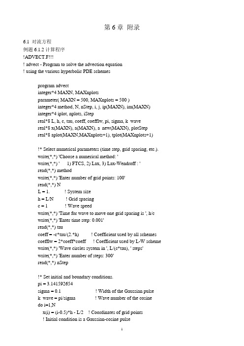
第6章附录6.1 对流方程例题6.1.2计算程序!ADVECT.F!!!! advect - Program to solve the advection equation! using the various hyperbolic PDE schemesprogram advectinteger*4 MAXN, MAXnplotsparameter( MAXN = 500, MAXnplots = 500 )integer*4 method, N, nStep, i, j, ip(MAXN), im(MAXN)integer*4 iplot, nplots, iStepreal*8 L, h, c, tau, coeff, coefflw, pi, sigma, k_wavereal*8 x(MAXN), a(MAXN), a_new(MAXN), plotStepreal*8 aplot(MAXN,MAXnplots+1), tplot(MAXnplots+1)!* Select numerical parameters (time step, grid spacing, etc.).write(*,*) 'Choose a numerical method: 'write(*,*) ' 1) FTCS, 2) Lax, 3) Lax-Wendroff : 'read(*,*) methodwrite(*,*) 'Enter number of grid points: 100'read(*,*) NL = 1. ! System sizeh = L/N ! Grid spacingc = 1 ! Wave speedwrite(*,*) 'Time for wave to move one grid spacing is ', h/cwrite(*,*) 'Enter time step: 0.001'read(*,*) taucoeff = -c*tau/(2.*h) ! Coefficient used by all schemescoefflw = 2*coeff*coeff ! Coefficient used by L-W schemewrite(*,*) 'Wave circles system in ', L/(c*tau), ' steps'write(*,*) 'Enter number of steps: 300'read(*,*) nStep!* Set initial and boundary conditions.pi = 3.141592654sigma = 0.1 ! Width of the Gaussian pulsek_wave = pi/sigma ! Wave number of the cosinedo i=1,Nx(i) = (i-0.5)*h - L/2 ! Coordinates of grid pointsa(i) = cos(k_wave*x(i)) * exp(-x(i)**2/(2*sigma**2))enddo! Use periodic boundary conditionsdo i=2,(N-1)ip(i) = i+1 ! ip(i) = i+1 with periodic b.c.im(i) = i-1 ! im(i) = i-1 with periodic b.c.enddoip(1) = 2ip(N) = 1im(1) = Nim(N) = N-1!* Initialize plotting variables.iplot = 1 ! Plot counternplots = 50 ! Desired number of plotsplotStep = float(nStep)/nplotstplot(1) = 0 ! Record the initial time (t=0)do i=1,Naplot(i,1) = a(i) ! Record the initial stateenddo!* Loop over desired number of steps.do iStep=1,nStep!* Compute new values of wave amplitude using FTCS,! Lax or Lax-Wendroff method.if( method .eq. 1 ) then !!! FTCS method !!!do i=1,Na_new(i) = a(i) + coeff*( a(ip(i))-a(im(i)) )enddoelse if( method .eq. 2 ) then !!! Lax method !!!do i=1,Na_new(i) = 0.5*( a(ip(i))+a(im(i)) ) +& coeff*( a(ip(i))-a(im(i)) )enddoelse !!! Lax-Wendroff method !!!do i=1,Na_new(i) = a(i) + coeff*( a(ip(i))-a(im(i)) ) +& coefflw*( a(ip(i))+a(im(i))-2*a(i) ) enddoendifa(i) = a_new(i) ! Reset with new amplitude valuesenddo!* Periodically record a(t) for plotting.if( (iStep-int(iStep/plotStep)*plotStep) .lt. 1 ) theniplot = iplot+1tplot(iplot) = tau*iStepdo i=1,Naplot(i,iplot) = a(i) ! Record a(i) for plotingenddowrite(*,*) iStep, ' out of ', nStep, ' steps completed'endifenddonplots = iplot ! Actual number of plots recorded!* Print out the plotting variables: x, a, tplot, aplotopen(11,file='x.txt',status='unknown')open(12,file='a.txt',status='unknown')open(13,file='tplot.txt',status='unknown')open(14,file='aplot.txt',status='unknown')do i=1,Nwrite(11,*) x(i)write(12,*) a(i)do j=1,(nplots-1)write(14,1001) aplot(i,j)enddowrite(14,*) aplot(i,nplots)enddodo i=1,nplotswrite(13,*) tplot(i)enddo1001 format(e12.6,', ',$) ! The $ suppresses the carriage return stopend!***** To plot in MATLAB; use the script below ******************** !load x.txt; load a.txt; load tplot.txt; load aplot.txt;!%* Plot the initial and final states.!figure(1); clf; % Clear figure 1 window and bring forward!plot(x,aplot(:,1),'-',x,a,'--');!legend('Initial','Final');!pause(1); % Pause 1 second between plots!%* Plot the wave amplitude versus position and time!figure(2); clf; % Clear figure 2 window and bring forward!mesh(tplot,x,aplot);!ylabel('Position'); xlabel('Time'); zlabel('Amplitude');!view([-70 50]); % Better view from this angle!****************************************************************** ================================================6.2 抛物形方程例题6.2.2计算程序!!!!dftcs.f!!!!!!!!!!! dftcs - Program to solve the diffusion equation! using the Forward Time Centered Space (FTCS) scheme.program dftcsinteger*4 MAXN, MAXnplotsparameter( MAXN = 300, MAXnplots = 500 )integer*4 N, i, j, iplot, nStep, plot_step, nplots, iStepreal*8 tau, L, h, kappa, coeff, tt(MAXN), tt_new(MAXN)real*8 xplot(MAXN), tplot(MAXnplots), ttplot(MAXN,MAXnplots)!* Initialize parameters (time step, grid spacing, etc.).write(*,*) 'Enter time step: 0.0001'read(*,*) tauwrite(*,*) 'Enter the number of grid points: 50 'read(*,*) NL = 1. ! The system extends from x=-L/2 to x=L/2h = L/(N-1) ! Grid sizekappa = 1. ! Diffusion coefficientcoeff = kappa*tau/h**2if( coeff .lt. 0.5 ) thenwrite(*,*) 'Solution is expected to be stable'elsewrite(*,*) 'WARNING: Solution is expected to be unstable'endif!* Set initial and boundary conditions.do i=1,Ntt(i) = 0.0 ! Initialize temperature to zero at all pointstt_new(i) = 0.0enddo!! The boundary conditions are tt(1) = tt(N) = 0!! End points are unchanged during iteration!* Set up loop and plot variables.iplot = 1 ! Counter used to count plotsnStep = 300 ! Maximum number of iterationsplot_step = 6 ! Number of time steps between plots nplots = nStep/plot_step + 1 ! Number of snapshots (plots)do i=1,Nxplot(i) = (i-1)*h - L/2 ! Record the x scale for plotsenddo!* Loop over the desired number of time steps.do iStep=1,nStep!* Compute new temperature using FTCS scheme.do i=2,(N-1)tt_new(i) = tt(i) + coeff*(tt(i+1) + tt(i-1) - 2*tt(i))enddodo i=2,(N-1)tt(i) = tt_new(i) ! Reset temperature to new valuesenddo!* Periodically record temperature for plotting.if( mod(iStep,plot_step) .lt. 1 ) then ! Every plot_step stepsdo i=1,N ! record tt(i) for plottingttplot(i,iplot) = tt(i)enddotplot(iplot) = iStep*tau ! Record time for plotsiplot = iplot+1endifenddonplots = iplot-1 ! Number of plots actually recorded!* Print out the plotting variables: tplot, xplot, ttplotopen(11,file='tplot.txt',status='unknown')open(12,file='xplot.txt',status='unknown')open(13,file='ttplot.txt',status='unknown')do i=1,nplotswrite(11,*) tplot(i)enddowrite(12,*) xplot(i)do j=1,(nplots-1)write(13,1001) ttplot(i,j)enddowrite(13,*) ttplot(i,nplots)enddo1001 format(e12.6,', ',$) ! The $ suppresses the carriage returnstopend!***** To plot in MATLAB; use the script below ********************!load tplot.txt; load xplot.txt; load ttplot.txt;!%* Plot temperature versus x and t as wire-mesh and contour plots.!figure(1); clf;!mesh(tplot,xplot,ttplot); % Wire-mesh surface plot!xlabel('Time'); ylabel('x'); zlabel('T(x,t)');!title('Diffusion of a delta spike');!pause(1);!figure(2); clf;!contourLevels = 0:0.5:10; contourLabels = 0:5;!cs = contour(tplot,xplot,ttplot,contourLevels); % Contour plot!clabel(cs,contourLabels); % Add labels to selected contour levels!xlabel('Time'); ylabel('x');!title('Temperature contour plot');!******************************************************************! program diffu_explicit.for! explicit methods for finite diffrencedimension T(51,51)real dx,dt,lamda,kp,Tmax,Tminopen(2,file='diffu_1.dat')dx=0.5dt=0.1kp=0.835lamda=kp*dt/dx/dxTmax=100.Tmin=0.imax=21write(*,*) 'lamda=',lamdado i=1,50do j=1,50T(i,j)=0.0do j=1,40T(1,j)=TmaxT(imax,j)=Tminend dodo j=1,40do i=2,20T(i,j+1)=T(i,j)+lamda*(T(i+1,j)-2.*T(i,j)+T(i-1,j)) end dowrite(2,222) (T(i,j),i=1,21)end do222 format(1x,21(2x,f18.10))end% diffu_explicit.mclc; clear all;nl = 20.; nt = 40;dx = 0.5; dt = 0.1; kp = 0.835;lamda = kp*dt/dx/dx;Tl = 0.; Tr = 100.;T = zeros(nl,nt);T(1,:) = Tl; T(nl,:)=Tr;for j=1:nt-1for i =2:nl-1T(i,j+1)=T(i,j)+lamda*(T(i+1,j)-2.*T(i,j)+T(i-1,j));endendsurf(T');xlabel('x');ylabel('time');zlabel('Temperature');title('explicit scheme');! diffu_implicit.for! implicit methods for finite diffrenceexternal tridparameter (imax=21,kmax=50)dimension t(imax),a(imax),b(imax),c(imax),r(imax),u(imax) real dx,dt,lamda,kp,tmax,tminopen(2,file='diffu_2.dat')dx=0.5lamda=kp*dt/dx/dxtmax=100.tmin=0.write(*,*) 'lamda=',lamdado i=2,imax-1! t(i)=tmax-(tmax-tmin)/(imax-1.)*(i-1.) t(i)=0.0end dot(1)=tmaxt(imax)=tmin! write(*,*) a(i),b(i),c(i)b(1)=1.c(1)=0.r(1)=t(1)a(imax)=0.b(imax)=1.r(imax)=t(imax)do i=2,imax-1a(i)=-lamdab(i)=1.+2.*lamdac(i)=-lamdar(i)=t(i)end dok=01 k=k+1call trid(a,b,c,r,u,imax)do i=1,imaxt(i)=u(i)r(i)=u(i)end dowrite(2,222) (t(i),i=1,imax)! write(*,222) (t(i),i=1,imax)if(k.lt.kmax) goto 1222 format(1x,21(2x,f18.12))endsubroutine trid(a,b,c,r,u,n)parameter (nmax=100)real gam(nmax),a(n),b(n),c(n),u(n),r(n)if (b(1)==0.) pause 'b(1)=0 in trid'bet=b(1)u(1)=r(1)/betdo j=2,ngam(j)=c(j-1)/betbet=b(j)-a(j)*gam(j)if (bet==0.) pause 'bet=0 in trid'u(j)=(r(j)-a(j)*u(j-1))/betend dodo j=n-1,1,-1u(j)=u(j)-gam(j+1)*u(j+1)end doend subroutine trid================================================== 6.3椭圆方程例题6.3.1计算程序! program overrelaxation.for! overrelaxation_iteration_methods for finite diffrence! of the 2d_Laplacian difference equationparameter(imax=25,jmax=25,pi=3.1415926)dimension T(imax,jmax),a(imax,jmax),& qx(imax,jmax),qy(imax,jmax),q(imax,jmax),an(imax,jmax) real lamda,Tu,Td,Tl,Tr,kpx,kpy,dx,dyopen(2,file='overrelaxation.dat')open(3,file='q.dat')lamda=1.5;Tu=100.;Tl=75.;Tr=50.;Td=0.;dx=1.;dy=1.;kmax=9 kpx=-0.49/2./dx;kpy=-0.49/2./dydo i=1,imaxdo j=1,jmaxT(i,j)=0.0end doend doT(1,1)=0.5*(Td+Tl) ;T(1,jmax)=0.5*(Tl+Tu)T(imax,jmax)=0.5*(Tu+Tr);T(imax,1)=0.5*(Tr+Td)do j=2,jmax-1T(1,j)=Tl; T(imax,j)=Trend dodo i=2, imax-1T(i,1)=Td; T(i,jmax)=Tuend dok=0do i=2,imax-1do j=2,jmax-1a(i,j)=T(i,j)T(i,j)=0.25*(T(i+1,j)+T(i-1,j)+T(i,j+1)+T(i,j-1))T(i,j)=lamda*T(i,j)+(1.-lamda)*a(i,j)end doend doep=abs((T(2,2)-a(2,2))/T(2,2))if(k.lt.kmax) goto 5write(*,*) 'ep=',epdo j=1,jmaxwrite(2,222) (T(i,j),i=1,imax)end do222 format(1x,25(2x,f14.10))do i=2,imax-1do j=2,jmax-1qx(i,j)=kpx*(T(i+1,j)-T(i-1,j))qy(i,j)=kpy*(T(i,j+1)-T(i,j-1))q(i,j)=sqrt(qx(i,j)*qx(i,j)+qy(i,j)*qy(i,j))if(qx(i,j).gt.0.) thenan(i,j)=atan(qy(i,j)/qx(i,j))elsean(i,j)=atan(qy(i,j)/qx(i,j))+piend ifend doend dodo j=2,jmax-1do i=2,imax-1! write(3,333) dx*(i-1),dy*(j-1),an(i,j),q(i,j)write(3,333) dx*(i-1),dy*(j-1),qx(i,j),qy(i,j)end doend do333 format(1x,4(2x,f18.12))End================================================= 例题6.3.2计算程序!!!!xadi.f90!!!!!program xadiuse AVDefuse DFLibparameter(n=19)real aj(n),bj(n),cj(n)integer statusreal T(0:n,0:n),TT(0:n,0:n)real lamda,Tu,Td,Tl,Tr,dx,dy,dt,kaopen(2,file='T3.dat')Tu=100.;Tl=75.;Tr=50.;Td=0.;dx=1.;dy=1.;kmax=10;dt=1.ka=0.835; lamda=ka*dt/(dx*dx)write(*,*) 'lamda=',lamdaT = 0.T(0,:) = Tl; T(n,:) =TrT(:,0) = Td; T(:,n) =TuT(0,0)=0.5*(Td+Tl);T(0,n)=0.5*(Tl+Tu)T(n,n)=0.5*(Tu+Tr);T(n,0)=0.5*(Tr+Td)! 系数矩阵赋值aj(:)=-lamda; ai(:)=lamdabj(:)= 2.*(1.+lamda); bi(:)=2.*(1-lamda)cj(:)=-lamda; ci(:)=lamdacall faglStartWatch(T, status)! 相当于随时间演化do k=1,kmaxdo i=1,n-1do j=1,n-1r(j)=ai(i)*T(i-1,j)+bi(i)*T(i,j)+ci(i)*T(i+1,j)end dor(1)=r(1)-aj(1)*T(i,0)r(n-1)=r(n-1)-cj(n-1)*T(i,n)call tridag(aj,bj,cj,r,u,n-1)do j=1,n-1T(i,j)=u(j)end doend do! 将矩阵T转置计算x方向call reverse(n,T,TT)do i=1,n-1do j=1,n-1r(j)=ai(i)*TT(i-1,j)+bi(i)*TT(i,j)+ci(i)*TT(i+1,j) end dor(1)=r(1)-aj(1)*TT(i,0)r(n-1)=r(n-1)-cj(n-1)*TT(i,n)call tridag(aj,bj,cj,r,u,n-1)do j=1,n-1TT(i,j)=u(j)end doend docall reverse(n,TT,T)call faglUpdate(T, status)call faglShow(T, status)end dopausecall faglClose(T, status)call faglEndWatch(T, status)do j=0,nwrite(2,222) (T(i,j),i=0,n)end do222 format(1x,20(2x,f14.10))endSUBROUTINE tridag(a,b,c,r,u,n)INTEGER n,NMAXREAL a(n),b(n),c(n),r(n),u(n)PARAMETER (NMAX=500)INTEGER jREAL bet,gam(NMAX)if(b(1).eq.0.)pause 'tridag: rewrite equations'bet=b(1)u(1)=r(1)/betdo 11 j=2,ngam(j)=c(j-1)/betbet=b(j)-a(j)*gam(j)if(bet.eq.0.)pause 'tridag failed'u(j)=(r(j)-a(j)*u(j-1))/bet11 continuedo 12 j=n-1,1,-1u(j)=u(j)-gam(j+1)*u(j+1)12 continuereturnENDSUBROUTINE REVERSE(n,T,TT) integer n,i,jreal T(0:n,0:n),TT(0:n,0:n)do i=0,ndo j=0,nTT(i,j)=T(j,i)end doend doreturnend================================================6.4 非线性偏微分方程% gasdynamincs_lw_1.mclc; clear all;xmin=-1.; xmax=1.; nx=101; h=(xmax-xmin)/(nx-1);r=0.9; cad=0.; time=0.; gamma=1.4; bcl=1.; bcr=1.;fprintf(' Space step - %f \n',h); fprintf(' \n');dd(1:nx)=zeros(1,nx); ud(1:nx)=zeros(1,nx); pd(1:nx)=zeros(1,nx);x(1:nx)=xmin+((1:nx)-1)*h;% Test 1te=' ( Test 1 )';rol=1.; ul=0.; pl=1.;ror=0.125; ur=0.; pr=0.1;tp=5.5;% Test 3%te=' ( Test 3 )';%rol=0.1; ul=0.; pl=1.;%ror=1.; ur=0.; pr=100.;%tp=0.05;% Initial conditionsdd(1:(nx-1)/2+1)=rol; ud(1:(nx-1)/2+1)=ul; pd(1:(nx-1)/2+1)=pl;dd((nx-1)/2+2:nx)=ror;ud((nx-1)/2+2:nx)=ur; pd((nx-1)/2+2:nx)=pr;[d,u,p,e,time]=lw_gasdynamics(dd,ud,pd,h,nx,r,cad,tp,gamma,bcl,bcr);% Exact solutionfor n=1:nx[density, velocity, pressure]=riemann(x(n),time,rol,ul,pl,ror,ur,pr,gamma);de(n)=density; ue(n)=velocity; pe(n)=pressure;ee(n)=pressure/((gamma-1.)*density);endfigure(1);plot(x,de,'k-',x,d,'k--');xlabel(' x ');ylabel(' density ');title([' Example 6.1 ',te]);figure(2);plot(x,ue,'k-',x,u,'k--');xlabel(' x ');ylabel(' velocity ');title([' Example 6.1 ',te]);figure(3);plot(x,pe,'k-',x,p,'k--');xlabel(' x ');ylabel(' pressure ');title([' Example 6.1 ',te]);figure(4);plot(x,ee,'k-',x,e,'k--');xlabel(' x ');ylabel(' internal energy ');title([' Example 6.1 ',te]);clear all;% Lax-Wendroff scheme (gasdynamics)function [d,u,p,e,time]=lw_gasdynamics(dd,ud,pd,h,nx,r,cad,tp,gamma,bcl,bcr)sd(1,1:nx)=dd(1:nx);sd(2,1:nx)=dd(1:nx).*ud(1:nx);sd(3,1:nx)=pd(1:nx)/(gamma-1.)+0.5*(dd(1:nx).*ud(1:nx)).*ud(1:nx);si(1:3,1:nx+1)=zeros(3,nx+1); av(1:3,1:nx)=zeros(3,nx);time=0.;while time <= tpsta=max(abs(sd(2,:)./sd(1,:))+...sqrt(gamma*(gamma-1)*(sd(3,:)./sd(1,:)-0.5*(sd(2,:).*sd(2,:))./(sd(1,:).*sd(1,:)))));tau=r*h*sqrt(1.-2.*cad)/sta;time=time+tau; %fprintf(' time - %f \n',time);% first stepif bcl == 0sl1=sd(1,2); sl2=-sd(2,2); sl3=sd(3,2);elsesl1=sd(1,2); sl2=sd(2,2); sl3=sd(3,2);endgl(1)=sl2;gl(2)=(gamma-1.)*sl3+0.5*(3.-gamma)*sl2^2/sl1;gl(3)=sl2*(gamma*sl3-0.5*(gamma-1.)*sl2^2/sl1)/sl1;for n=1:nxif (n == 1)|(n == nx)av(:,n)=[ 0.; 0.; 0.;];elseav(:,n)=cad*(sd(:,n+1)-2.*sd(:,n)+sd(:,n-1));endsr1=sd(1,n); sr2=sd(2,n); sr3=sd(3,n);gr(1)=sr2;gr(2)=(gamma-1.)*sr3+0.5*(3.-gamma)*sr2^2/sr1;gr(3)=sr2*(gamma*sr3-0.5*(gamma-1.)*sr2^2/sr1)/sr1;si(1,n)=0.5*(sl1+sr1)-(gr(1)-gl(1))*tau*0.5/h;si(2,n)=0.5*(sl2+sr2)-(gr(2)-gl(2))*tau*0.5/h;si(3,n)=0.5*(sl3+sr3)-(gr(3)-gl(3))*tau*0.5/h;gl(:)=gr(:);sl1=sr1; sl2=sr2; sl3=sr3;endif bcr == 0sr1=sd(1,nx-1); sr2=-sd(2,nx-1); sr3=sd(3,nx-1);elsesr1=sd(1,nx-1); sr2=sd(2,nx-1); sr3=sd(3,nx-1);endgr(1)=sr2;gr(2)=(gamma-1.)*sr3+0.5*(3.-gamma)*sr2^2/sr1;gr(3)=sr2*(gamma*sr3-0.5*(gamma-1.)*sr2^2/sr1)/sr1;si(1,nx+1)=0.5*(sl1+sr1)-(gr(1)-gl(1))*tau*0.5/h;si(2,nx+1)=0.5*(sl2+sr2)-(gr(2)-gl(2))*tau*0.5/h;si(3,nx+1)=0.5*(sl3+sr3)-(gr(3)-gl(3))*tau*0.5/h;% second stepfl(1)=si(2,1);fl(2)=(gamma-1.)*si(3,1)+0.5*(3.-gamma)*si(2,1)^2/si(1,1);fl(3)=si(2,1)*(gamma*si(3,1)-0.5*(gamma-1.)*si(2,1)^2/si(1,1))/si(1,1);for n=2:nx+1fr(1)=si(2,n);fr(2)=(gamma-1.)*si(3,n)+0.5*(3.-gamma)*si(2,n)^2/si(1,n);fr(3)=si(2,n)*(gamma*si(3,n)-0.5*(gamma-1.)*si(2,n)^2/si(1,n))/si(1,n);su(:,n-1)=sd(:,n-1)-(fr(:)-fl(:))*tau/h+av(:,n-1);fl(:)=fr(:);endsd(:,1:nx)=su(:,1:nx);endd(1:nx)=su(1,1:nx); u(1:nx)=su(2,1:nx)./su(1,1:nx);p(1:nx)=(gamma-1.)*(su(3,1:nx)-0.5*(su(2,1:nx).*su(2,1:nx))./su(1,1:nx));e(1:nx)=(su(3,1:nx)-0.5*(su(2,1:nx).*su(2,1:nx))./su(1,1:nx))./su(1,1:nx);return;% Solves Riemann problem for ideal gas% r1, u1, p1 initial parameters for x<0% r2, u2, p2 initial parameters for x>0% rf, uf, pf solution at the point (x,t)% c1, c2 sound speeds for x<0 and for x>0% s1, sr velocties of the fronts of S(hock)W(ave)s% shl, shr velocties of the fronts of the heads of R(arefaction)Ws% stl, str velocties of the tails of RWsfunction [rf,uf,pf]=riemann(x,t,r1,u1,p1,r2,u2,p2,gamma)g(1)=0.5*(gamma-1.)/gamma; g(2)=0.5*(gamma+1.)/gamma; g(3)=2.*gamma/(gamma-1.); g(4)=2./(gamma-1.); g(5)=2./(gamma+1.); g(6)=(gamma-1.)/(gamma+1.);g(7)=0.5*(gamma-1.); g(8)=1./gamma; g(9)=gamma-1.;s=x/t;c1 = sqrt(p1/(r1*g(8)));c2 = sqrt(p2/(r2*g(8)));du=u2-u1;% Vacuum solutionuvac=g(4)*(c1+c2)-du;if uvac <= 0.disp(' Vacuum generated by given data');return;end% Apply Newton method% Initial guessespv=0.5*(p1+p2)-0.125*du*(r1+r2)*(c1+c2);pmin=min(p1,p2); pmax=max(p1,p2); qrat=pmax/pmin;if ( qrat <= 2. ) & ( pmin <= pv & pv <= pmax )p=max(1.0e-6,pv);elseif pv < pminpnu=c1+c2-g(7)*du;pde=c1/(p1^g(1))+c2/(p2^g(1));p=(pnu/pde)^g(3);elsegel=sqrt((g(5)/r1)/(g(6)*p1+max(1.0e-6,pv)));ger=sqrt((g(5)/r2)/(g(6)*p2+max(1.0e-6,pv)));p=(gel*p1+ger*p2-du)/(gel+ger); p=max(1.0e-6,p);endendp0=p; err=1.;while err > 1.0e-5if p <= p1prat=p/p1; fl=g(4)*c1*(prat^g(1)-1.); ffl=1./(r1*c1*prat^g(2));elsea=g(5)/r1; b=g(6)*p1; qrt=sqrt(a/(b+p));fl=(p-p1)*qrt; ffl=(1.-0.5*(p-p1)/(b+p))*qrt;endif p <= p2prat=p/p2; fr=g(4)*c2*(prat^g(1)-1.); ffr=1./(r2*c2*prat^g(2));elsea=g(5)/r2; b=g(6)*p2; qrt=sqrt(a/(b+p));fr=(p-p2)*qrt; ffr=(1.-0.5*(p-p2)/(b+p))*qrt;endp=p-(fl+fr+du)/(ffl+ffr);err=2.*abs(p-p0)/(p+p0); p0=p;endif p0 < 0.p0=1.0e-6;end% Velocity of CDu0=0.5*(u1+u2+fr-fl);if s <= u0if p0 <= p1shl=u1-c1;if s <= shlrf=r1; uf=u1; pf=p1; return;elsecml=c1*(p0/p1)^g(1); stl=u0-cml;if s > stlrf=r1*(p0/p1)^g(8); uf=u0; pf=p0; return;elseuf=g(5)*(c1+g(7)*u1+s); c=g(5)*(c1+g(7)*(u1-s));rf=r1*(c/c1)^g(4); pf=p1*(c/c1)^g(3);return;endendelsepml=p0/p1; sl=u1-c1*sqrt(g(2)*pml+g(1));if s <= slrf=r1; uf=u1; pf=p1; return;elserf=r1*(pml+g(6))/(pml*g(6)+1.); uf=u0; pf=p0; return;endendelseif p0 > p2pmr=p0/p2; sr=u2+c2*sqrt(g(2)*pmr+g(1));if s >= srrf=r2; uf=u2; pf=p2; return;elserf=r2*(pmr+g(6))/(pmr*g(6)+1.); uf=u0; pf=p0; return;endelseshr=u2+c2;if s >= shrrf=r2; uf=u2; pf=p2; return;elsecmr=c2*(p0/p2)^g(1); str=u0+cmr;if s <= strrf=r2*(p0/p2)^g(8); uf=u0; pf=p0; return;elseuf=g(5)*(-c2+g(7)*u2+s); c=g(5)*(c2-g(7)*(u2-s));rf=r2*(c/c2)^g(4); pf=p2*(c/c2)^g(3);return;endendendendreturn;%%%%%%%%% gasdynamics_Godunov.m%%%%%%%%%%%%%clc; clear all;xmin=-1.; xmax=1.; nx=101; h=(xmax-xmin)/(nx-1);r=0.9; gamma=1.4; bcl=1.; bcr=1.;fprintf('gasdynamics_godunov \n'); fprintf(' Space step - %f \n',h); fprintf(' \n'); dd(1:nx-1)=zeros(1,nx-1); ud(1:nx-1)=zeros(1,nx-1); pd(1:nx-1)=zeros(1,nx-1);x(1:nx)=xmin+((1:nx)-1)*h; xa=xmin+((1:nx-1)-0.5)*h;% Test 1te=' ( Test 1 )';rol=1.; ul=0.; pl=1.;ror=0.125; ur=0.; pr=0.1;tp=15.5;% Test 2%te=' ( Test 2 )';%rol=1.; ul=0.; pl=1000.;%ror=1.; ur=0.; pr=1.;%tp=0.024;% Test 3%te=' ( Test 3 )';%rol=0.1; ul=0.; pl=1.;%ror=1.; ur=0.; pr=100.;%tp=0.05;% Test 4%te=' ( Test 4 )';%rol=5.99924; ul=19.5975; pl=460.894;%ror=5.99242; ur=-6.19633; pr=46.0950;%tp=0.05;% Test 5%te=' ( Test 5 )';%rol=3.86; ul=-0.81; pl=10.33;%ror=1.; ur=-3.44; pr=1.;%tp=0.5;% Initial conditionsdd(1:(nx-1)/2)=rol; ud(1:(nx-1)/2)=ul; pd(1:(nx-1)/2)=pl;dd((nx-1)/2+1:nx-1)=ror;ud((nx-1)/2+1:nx-1)=ur; pd((nx-1)/2+1:nx-1)=pr;[d,u,p,e,time]=godunov_gasdynamics(dd,ud,pd,h,nx,r,tp,gamma,bcl,bcr);% Exact solutionfor n=1:nx[density, velocity, pressure]=riemann(x(n),time,rol,ul,pl,ror,ur,pr,gamma);de(n)=density; ue(n)=velocity; pe(n)=pressure;ee(n)=pressure/((gamma-1.)*density);endfigure(1);plot(x,de,'k-',xa,d,'ko');xlabel(' x ');ylabel(' density ');title([' Example 6.3 ',te]);figure(2);plot(x,ue,'k-',xa,u,'ko');xlabel(' x ');ylabel(' velocity ');figure(3);plot(x,pe,'k-',xa,p,'ko');xlabel(' x ');ylabel(' pressure ');figure(4);plot(x,ee,'k-',xa,e,'ko');xlabel(' x ');ylabel(' internal energy ');clear all;% Method of S. K. Godunovfunction [d,u,p,e,time]=godunov_gasdynamics(dd,ud,pd,h,nx,r,tp,gamma,bcl,bcr)g(1)=0.5*(gamma-1.)/gamma; g(2)=0.5*(gamma+1.)/gamma; g(3)=2.*gamma/(gamma-1.); g(4)=2./(gamma-1.); g(5)=2./(gamma+1.); g(6)=(gamma-1.)/(gamma+1.);g(7)=0.5*(gamma-1.); g(8)=1./gamma; g(9)=gamma-1.;sd(1,1:nx-1)=dd(1:nx-1);sd(2,1:nx-1)=dd(1:nx-1).*ud(1:nx-1);sd(3,1:nx-1)=pd(1:nx-1)/(gamma-1.)+0.5*(dd(1:nx-1).*ud(1:nx-1)).*ud(1:nx-1);time=0.;while time <= tpsta=max(abs(sd(2,:)./sd(1,:))+...sqrt(gamma*(gamma-1)*(sd(3,:)./sd(1,:)-0.5*(sd(2,:).*sd(2,:))./(sd(1,:).*sd(1,:)))));tau=r*h/sta;time=time+tau; %fprintf(' %f \n',time);if bcl == 0[f1,f2,f3]=flux_godunov(sd(1,1),-sd(2,1),sd(3,1),sd(1,1),sd(2,1),sd(3,1),g(:));else[f1,f2,f3]=flux_godunov(sd(1,1),sd(2,1),sd(3,1),sd(1,1),sd(2,1),sd(3,1),g(:));endfleft(1)=f1; fleft(2)=f2; fleft(3)=f3;for n=1:nx-2[f1,f2,f3]=flux_godunov(sd(1,n),sd(2,n),sd(3,n),sd(1,n+1),sd(2,n+1),sd(3,n+1),g(:));fright(1)=f1; fright(2)=f2; fright(3)=f3;su(:,n)=sd(:,n)-(fright(:)-fleft(:))*tau/h;fleft(:)=fright(:);endif bcr == 0[f1,f2,f3]=flux_godunov(sd(1,nx-1),sd(2,nx-1),sd(3,nx-1),sd(1,nx-1),-sd(2,nx-1),...sd(3,nx-1),g(:));else[f1,f2,f3]=flux_godunov(sd(1,nx-1),sd(2,nx-1),sd(3,nx-1),sd(1,nx-1),sd(2,nx-1),...sd(3,nx-1),g(:));endfright(1)=f1; fright(2)=f2; fright(3)=f3;su(:,nx-1)=sd(:,nx-1)-(fright(:)-fleft(:))*tau/h;sd(:,1:nx-1)=su(:,1:nx-1);endd(1:nx-1)=su(1,1:nx-1); u(1:nx-1)=su(2,1:nx-1)./su(1,1:nx-1);p(1:nx-1)=(gamma-1.)*(su(3,1:nx-1)-0.5*(su(2,1:nx-1).*su(2,1:nx-1))./su(1,1:nx-1));e(1:nx-1)=(su(3,1:nx-1)-0.5*(su(2,1:nx-1).*su(2,1:nx-1))./su(1,1:nx-1))./su(1,1:nx-1); return;% Solves Riemann problem for ideal gas% r1, u1, p1 initial parameters for x<0% r2, u2, p2 initial parameters for x>0% rf, uf, pf solution at the point (x,t)% c1, c2 sound speeds for x<0 and for x>0% s1, sr velocties of the fronts of S(hock)W(ave)s% shl, shr velocties of the fronts of the heads of R(arefaction)Ws% stl, str velocties of the tails of RWsfunction [rf,uf,pf]=riemann(x,t,r1,u1,p1,r2,u2,p2,gamma)g(1)=0.5*(gamma-1.)/gamma; g(2)=0.5*(gamma+1.)/gamma; g(3)=2.*gamma/(gamma-1.);g(7)=0.5*(gamma-1.); g(8)=1./gamma; g(9)=gamma-1.;s=x/t;c1 = sqrt(p1/(r1*g(8)));c2 = sqrt(p2/(r2*g(8)));du=u2-u1;% Vacuum solutionuvac=g(4)*(c1+c2)-du;if uvac <= 0.disp(' Vacuum generated by given data');return;end% Apply Newton method% Initial guessespv=0.5*(p1+p2)-0.125*du*(r1+r2)*(c1+c2);pmin=min(p1,p2); pmax=max(p1,p2); qrat=pmax/pmin;if ( qrat <= 2. ) & ( pmin <= pv & pv <= pmax )p=max(1.0e-6,pv);elseif pv < pminpnu=c1+c2-g(7)*du;pde=c1/(p1^g(1))+c2/(p2^g(1));p=(pnu/pde)^g(3);elsegel=sqrt((g(5)/r1)/(g(6)*p1+max(1.0e-6,pv)));ger=sqrt((g(5)/r2)/(g(6)*p2+max(1.0e-6,pv)));p=(gel*p1+ger*p2-du)/(gel+ger); p=max(1.0e-6,p);endendp0=p; err=1.;while err > 1.0e-5if p <= p1prat=p/p1; fl=g(4)*c1*(prat^g(1)-1.); ffl=1./(r1*c1*prat^g(2));elsea=g(5)/r1; b=g(6)*p1; qrt=sqrt(a/(b+p));fl=(p-p1)*qrt; ffl=(1.-0.5*(p-p1)/(b+p))*qrt;endif p <= p2prat=p/p2; fr=g(4)*c2*(prat^g(1)-1.); ffr=1./(r2*c2*prat^g(2));a=g(5)/r2; b=g(6)*p2; qrt=sqrt(a/(b+p));fr=(p-p2)*qrt; ffr=(1.-0.5*(p-p2)/(b+p))*qrt;endp=p-(fl+fr+du)/(ffl+ffr);err=2.*abs(p-p0)/(p+p0); p0=p;endif p0 < 0.p0=1.0e-6;end% Velocity of CDu0=0.5*(u1+u2+fr-fl);if s <= u0if p0 <= p1shl=u1-c1;if s <= shlrf=r1; uf=u1; pf=p1; return;elsecml=c1*(p0/p1)^g(1); stl=u0-cml;if s > stlrf=r1*(p0/p1)^g(8); uf=u0; pf=p0; return;elseuf=g(5)*(c1+g(7)*u1+s); c=g(5)*(c1+g(7)*(u1-s));rf=r1*(c/c1)^g(4); pf=p1*(c/c1)^g(3);return;endendelsepml=p0/p1; sl=u1-c1*sqrt(g(2)*pml+g(1));if s <= slrf=r1; uf=u1; pf=p1; return;elserf=r1*(pml+g(6))/(pml*g(6)+1.); uf=u0; pf=p0; return;endendelseif p0 > p2pmr=p0/p2; sr=u2+c2*sqrt(g(2)*pmr+g(1));if s >= srrf=r2; uf=u2; pf=p2; return;rf=r2*(pmr+g(6))/(pmr*g(6)+1.); uf=u0; pf=p0; return;endelseshr=u2+c2;if s >= shrrf=r2; uf=u2; pf=p2; return;elsecmr=c2*(p0/p2)^g(1); str=u0+cmr;if s <= strrf=r2*(p0/p2)^g(8); uf=u0; pf=p0; return;elseuf=g(5)*(-c2+g(7)*u2+s); c=g(5)*(c2-g(7)*(u2-s));rf=r2*(c/c2)^g(4); pf=p2*(c/c2)^g(3);return;endendendendreturn;% Solves Riemann problem and computes fluxes for method of S. K. Godunov% r1, u1, p1 parameters in left cell% r2, u2, p2 parameters in right cell% rf, uf, pf parameters on the interface% c1, c2 sound speeds in left and right cells% s1, sr velocties of the fronts of S(hock)W(ave)s% shl, shr velocties of the fronts of the heads of R(arefaction)Ws% stl, str velocties of the tails of RWsfunction [f1,f2,f3]=flux_godunov(sl1,sl2,sl3,sr1,sr2,sr3,g)r1=sl1; u1=sl2/r1; p1=(1./g(8)-1.)*(sl3-0.5*sl2*u1);r2=sr1; u2=sr2/r2; p2=(1./g(8)-1.)*(sr3-0.5*sr2*u2);% sound speeds in left and right cellsc1 = sqrt(p1/(r1*g(8)));c2 = sqrt(p2/(r2*g(8)));du=u2-u1;% Vacuum solution。
偏微分方程数值解PPT课件

t
t
n j
tn j1
x x
EXCEL
0.01, x 0.1
t n1 j
t
n j
2(TW
t
n j
)
3
t
n j
t
n j1
x
t n1 j
0.02TW
0.68t
n j
0.3t
n j1
此微分方程,是在不考虑流体本身热传 导时的套管传热微分方程.由计算结果可 知,当计算的时间序列进行到72时,传 热过程已达到稳态,各点上的温度已不 随时间的增加而改变。如果改变套管长 度或传热系数,则达到稳态的时间亦会 改变。
b2 4ac 0 b2 4ac 0 b2 4ac 0
• 物理实际问题的归类:
• 波动方程(双曲型)一维弦振动模型:
2u t 2
2
2u x 2
• 热传导方程(抛物线型)一维线性热传导方程
u t
2u x 2
• 拉普拉斯方程(椭圆型ux22)稳态y2u2 静 电0 场或稳态温度分布场)
第4页/共32页
un i 1
b
un i1
uin
x
f (ix, nt)
ui0
(i x )
un m1
umn
x
0
u0n 1(nt )
(i 1,2, ,m) (n 0,1, 2, ) (n 0,1,2, )
第13页/共32页
一维流动热传导方程
将上式进行处理得到:
un1 i
t
f
(ix, nt )
(a2
t (x)2
1的)偏t )
微
分
采
用
向
后
欧
第十章偏微分方程的数值解.doc
第十章偏微分方程的数值解第十章偏微分方程的数值解求解偏微分方程问题非常困难。
除了少数特殊情况,在大多数情况下很难找到准确的解决方案。
因此,近似解更重要。
本章只介绍求解各种典型偏微分方程定解问题的差分方法。
(1)差分方法的基本概念 1.1几种偏微分方程固定解的椭圆方程;最典型和最简单的形式是泊松方程。
特别是,在那个时候,它是拉普拉斯方程,也称为调和方程。
泊松方程的第一个边值问题是一个有边界的有界区域,一条分段光滑曲线,称为固定解区域,以及已知的连续函数。
第二类和第三类边界条件可以统一表示为边界的外法线方向。
当时,这是第二种边界条件,当时,这是第三种边界条件。
抛物线方程:在最简单的形式中,一维热传导方程可以有两种不同类型的定解:初值问题初边值问题在初边值问题中,是一个已知的函数,满足连接条件,边界条件称为第一类边界条件。
第二个和第三个边界条件在其中。
当时,它是第二类边界条件,否则它被称为第三类边界条件。
双曲线方程:的最简单形式是一阶双曲线方程。
物理学中常见的一维振动和波动问题可以用二阶波动方程来描述,二阶波动方程是双曲方程的一种典型形式。
方程的初值问题是一个边界条件,一般有三种类型。
最简单的初边值问题是1.2差分法。
差分法的基本概念也称为有限差分法或网格法。
它是求解偏微分方程定解问题数值解最广泛使用的方法之一。
其基本思想是:首先,对求解区域进行网格划分,用一组有限离散点(网格点)代替自变量的连续变化区域。
问题中出现的连续变量的函数被定义在网格点上的离散变量的函数所代替。
通过用网格点上函数的差商代替导数,将具有连续变量的偏微分方程的固定解问题转化为只有有限个未知数的代数方程(称为差分格式)。
当网格为无穷大时,如果差分格式有解,并且其解收敛于原微分方程的解,则差分格式的解作为原问题的近似解(数值解)。
因此,在用差分法求偏微分方程的定解时,通常需要解决以下问题:(1)选择网格;(2)选择微分方程和固定解条件的差分逼近,列出差分格式;(3)求解差分方案;(4)讨论微分方程差分格式解的收敛性和误差估计。
《偏微分方程》课程大纲
《偏微分⽅程》课程⼤纲《偏微分⽅程》课程⼤纲⼀、课程简介教学⽬标:“偏微分⽅程”是重要的数学基础课程,它在数学的其它分⽀和⾃然科学与⼯程技术中的⼴泛应⽤是众所周知的。
本课程将尽可能地结合物理背景,系统地对⼏类典型⽅程数学结构、求解⽅法、解的性质以及物理意义进⾏详细阐述,为学⽣⽇后的学习和⼯作打下坚实的基础,提供强有⼒的⼯具,并为进⼀步了解和应⽤现代偏微分⽅程的有关内容提供重要帮助。
主要内容:1. 了解⼏类典型⽅程及其定解条件的物理背景2.掌握⽅程的分类及其化简⽅法3. 熟练掌握各类⽅程的求解⽅法(包括具有普适性的⽅法,如分离变量法,Fourier变换法和Green函数法等,以及针对某类⽅程的特定⽅法,如特征线法)4. 会⽤⼀些基本⽅法(如能量积分法、极值原理等)讨论解的性质并掌握解的重要性质⼆、教学内容(其中带*的部分可能随堂调整)第⼀章引论主要内容:1、偏微分⽅程简介a)偏微分⽅程的历史、现状和⽤途b)什么是偏微分⽅程?介绍有关偏微分⽅程基本概念和研究内容c)例⼦:简单⽽多样的例⼦帮助学⽣初步了解偏微分⽅程2、⼆阶线性偏微分⽅程的分类和特征理论a)两个⾃变量的⼆阶线性偏微分⽅程的分类与化简,椭圆型、双曲型和抛物型的标准形式与典型例⼦,混合型⽅程b)多个⾃变量的⼆阶线性偏微分⽅程⽅程的分类及其例⼦c)⼆阶线性⽅程的特征理论*3、四类典型⽅程的数学模型:包括波动⽅程、热传导⽅程、调和⽅程、和⼀阶⽅程4、其他预备知识:线性⽅程的叠加原理、Sturm-Liouville原理*重点与难点:通过化标准型将⼆阶⽅程进⾏分类、特征的概念(这是偏微分⽅程中最基本也是最重要的概念)、各类⽅程及其定解条件的物理意义第⼆章波动⽅程主要内容:1、弦振动⽅程Cauchy问题的存在性:D’Alembert求解公式,传播波,依赖区域、决定区域和影响区域,特征线法(⾏波法)的其他应⽤和例⼦,Duhamel齐次化原理及其物理解释2、弦振动⽅程初边值问题的存在性:分离变量法求解齐次问题及解的存在性讨论,分离变量法求解的物理意义,多种边界条件的例⼦,⾮齐次⽅程的情形,⾮齐次边界条件的情形,⾼维波动⽅程分离变量法的例⼦3、⾼维波动⽅程Cauchy问题的求解:三维波动⽅程的球平均法,⼆维波动⽅程的降维法4、波的传播与衰减:依赖区域、决定区域和影响区域,Huygens原理与波的弥散,波动⽅程解的长时间性态5、能量不等式与唯⼀性和稳定性:初边值问题解的唯⼀性和稳定性,Cauchy问题解的唯⼀性和稳定性重点与难点:针对于波动⽅程:特征线与特征锥、特征线⽅法、波的有限传播速度;适⽤于各种⽅程的普遍⽅法:能量积分⽅法、分离变量法第三章热传导⽅程主要内容:1、求解初边值问题的分离变量法:⼀维情形,⾼维的例⼦2、Cauchy问题解的存在性:Fourier变换及其基本性质,⽤Fourier变换法求解Cauchy 问题及解的存在性讨论,Fourier变换法的其他应⽤3、极值原理与唯⼀性和稳定性:有界区域的极值原理,⽆界区域的极值原理,初边值问题解的唯⼀性和稳定性,Cauchy问题解的唯⼀性和稳定性4、解的渐近性态:初边值问题解的渐近性态,Cauchy问题解的渐近性态重点与难点:Fourier变换⽅法、极值原理、关注与波动⽅程的区别第四章调和⽅程主要内容:1、调和函数的基本性质:Green公式,Neumann问题解的⾃由度与可解性条件,调和⽅程的基本解,变分原理、基本积分公式,平均值定理,极值原理、边值问题解的唯⼀性和稳定性2、Green函数:定义和性质,⽤静电源像法求⼀些特殊区域的Green函数,⼀般单连通区域的Green函数,⽤Green函数法求解调和⽅程与Poisson⽅程3、调和函数的进⼀步性质―――Harnack定理,可去奇点定律,解析性定理、强极值原理、Neumann边值问题解的唯⼀性。
(完整版)偏微分方程课程教学大纲
4
上课
作业
掌握思想
测验一
波动方程的有限传播速度
2
上课
作业
掌握波动方程的特性
一维波动方程初边值问题
4
上课
作业
掌握分离变量法
波动方程的能量方法
4
上课
作业
掌握PDE能量方法
期中考试
热方程的Cauchy问题
4
上课
作业
掌握Fourier变换及基本解思想
热ቤተ መጻሕፍቲ ባይዱ程的初边值问题
2
上课
作业
掌握分离变量法
在该课程中,我们将重点讲解刻画粒子输运、波的传播、温度变化及物理场论的输运方程、波动方程、热方程及Laplace方程的理论与方法,从而了解双曲型、抛物型及椭圆型三类偏微分方程的特性及基本分析思路,为进一步学习与研究打下一定的基础。
*课程简介(Description)
In this course,we shall teach students how to formulate the partial differential equation models based on certain elementary laws in physics and mechanics, then purpose some analytic methods for studying qualitative and quantitative properties of solutions to several important kinds of partial differential equations,which could inspire students to understand some basic idea of modern methods and theories of partial differential equations。 By solving the explicit solutions of PDEs, it can explain some important phenomena in physics and mechanics, which could inspire the students to study further。
《微分方程数值解》课程简介
《微分方程数值解》课程简介06191140 微分方程数值解 3Numerical Methods for Differential Equations3-0预修要求:数学分析,高等代数或线性代数, 常微分方程面向对象:数学系信息与计算科学专业三、四年级本科生内容简介:《微分方程数值解法》包括常微分方程初值问题的差分格式的构造和性态分析;椭圆型方程的差分方法;抛物型方程的差分方法;双曲型方程的差分方法;通过本课程的学习,使学生掌握求解微分方程数值解的基本方法,能够根据具体的微分方程选用合适的计算方法。
推荐教材或主要参考书:《微分方程数值解法》,李荣华等,高等教育出版社。
《微分方程数值方法》,胡健伟,汤怀民著,科学出版社。
《初值问题的差分方法》,R.D.Richtmyer and K.W.Morton著,袁国兴等译,中山大学出版社。
《偏微分方程数值方法》,陆金甫,关治,清华大学出版社《微分方程数值解》教学大纲06191140 微分方程数值解 3Numerical Methods for Differential Equations3-0预修要求:数学分析,高等代数或线性代数, 常微分方程面向对象:数学系信息与计算科学专业三、四年级本科生一、课程的教学目的和基本要求本课程是为数学系信息与计算科学专业开设的专业课。
本课程为3学分,上课时间大约为16×3=48学时,春夏或秋冬学期完成。
通过本课程的学习,要使学生掌握常微分方程初值问题的单步和多步差分方法,椭圆型微分方程的差分方法,抛物型微分方程的差分方法,双曲型微分方程的差分方法,以及与之相关的理论问题。
学会分析各种计算方法的收敛条件和收敛速度。
二、课程主要内容及学时分配(一)常微分方程的初值问题(15学时)1.引论。
2.Euler方法。
3.线性多步方法。
4.稳定性、收敛性和误差估计。
5.多步方法的计算。
6.预估—校正算法。
7.Runge—Kutta方法。
《偏微分方程数值解》课程教学大纲
《偏微分方程数值解》课程教学大纲《偏微分方程数值解》课程教学大纲课程名称:偏微分方程数值解课程代码:MA309学分 / 学时:4学分 / 64学时适用专业:数学系和与科学计算相关的专业先修课程:偏微分方程,科学计算(I)后续课程:科学计算(II),科学计算选讲开课单位:理学院数学系一、课程性质和教学目标(需明确各教学环节对人才培养目标的贡献)课程性质:本课程是理学院数学系的一门重要专业基础课程,其主要任务是通过理论学习和上机实算,使学生掌握偏微分方程数值解的基本概念,基本方法和基本原理。
教学目标:重点介绍偏微分方程数值解的有限差分法、和有限元方法,培养学生以计算机为工具,通过数学建模、理论分析与数值求解等步骤定量化解决实际问题的能力。
本课程各教学环节对人才培养目标的贡献见下表。
知识能力素质要求各教学环节的贡献度课堂讲授课堂讨论自学小组大作业作业考试课堂整体贡献度知识知识体系完整掌握求解线性偏微分方程的有限差分方法,掌握变分原理和有限元方法的基本知识√√√能力清晰思考和用语言文字准确表达的能力√ √√ √ √√√√√ √√ √√ 发现、分析和解决问题的能力√√ √√ √√ √√√√√ √√ √√ 批判性思考和创造性工作的能力√√ √√√√√ √√√√√ √√ √√ 与不同类型的人合作共事的能力√ √ √√至少一种外语的应用能力√ √ 终生学习的能力√√ √√ √√ 组织管理能力√ √ 获取整理信息的能力* √ √√ √√√√√ √√ √√素质志存高远、意志坚强√ √ √√ √ 刻苦务实、精勤进取√√ √√ √√ √√ √√ √√ √√ 身心和谐、视野开阔√ √ √√ √√ 思维敏捷、乐于创新√√ √√ √ √√√√ √√ √√二、课程教学内容及学时分配(含实践、自学、作业、讨论等的内容及要求)教学内容学时课堂教学讨论作业及要求自学及要求团组大作业及要求第一章总论微分方程数学模型及举例;微分方程数值解的重要意义和基本问题。
- 1、下载文档前请自行甄别文档内容的完整性,平台不提供额外的编辑、内容补充、找答案等附加服务。
- 2、"仅部分预览"的文档,不可在线预览部分如存在完整性等问题,可反馈申请退款(可完整预览的文档不适用该条件!)。
- 3、如文档侵犯您的权益,请联系客服反馈,我们会尽快为您处理(人工客服工作时间:9:00-18:30)。
中国海洋大学本科生课程大纲
课程属性:公共基础/通识教育/学科基础/专业知识/工作技能,课程性质:必修、选修
一、课程介绍
1.课程描述:
本课程介绍数值求解偏微分方程的基本方法及相关的理论基础。
本课程针对数学类专业高年级(三年级)本科生开设。
课程基本内容包括:有限差分方法、差分格式的稳定性、收敛性分析;变分原理,Galerkin有限元方法等。
通过对模型问题的基本数值方法进行分析,阐明构造数值方法的基本思想和技巧。
通过本课程学习,使学生了解并掌握数值求解偏微分方程的基本思想、基本概念和基本理论(数值格式的相容性、稳定性、收敛性及误差估计等),能够运用算法语言对所学数值方法编制程序在计算机上运行实施并对数值结果进行分析。
培养学生理论联系实际,解决实际问题的能力和兴趣。
2.设计思路:
偏微分方程是应用数学的核心内容,在其他科学、技术领域具有广泛深入的应用。
掌握偏微分方程的基础理论及求解方法是数学类专业本科生培养的基本要求。
本课程是在数学物理方程课程基础上开设的延展应用型课程,是一门数值分析理论与实践应用高度融合的专业课。
课程引导学生通过数值方法探讨和理解应用数学工具解决实际
- 6 -
问题的途径及理论分析框架。
学习本课程需要学生掌握了“数学分析”、“数学物理方程”、“数值分析”及“泛函分析”的核心基本内容。
课程内容安排分为有限差分方法和有限元方法两个单元模块,这是目前应用最广泛、理论发展最完善的两类数值方法,两者既有关联又有本质区别,能够体现偏微分方程数值解法的基本特征。
首先介绍有限差分方法。
有限差分方法是近似求解偏微分方程的应用最广泛的数值方法,以对连续的“导数(微分)”进行离散的“差分”近似为基本出发点,利用Fourier 分析及数值分析的基本理论,讨论椭圆、抛物、双曲等三类典型偏微分方程近似求解方法及近似方法的数学理论分析。
有限元方法是20世纪中期发展起来的基于变分原理的数值方法,具有更直接的物理背景含义,因而受到力学、工程等应用领域广泛的关注和应用。
有限元方法与有限差分法虽然在思想方法上有本质区别,但在一定条件下具有等价性。
课程将以实际问题为引导,阐述变分原理的基本理论和实际应用背景,介绍Galerkin 近似和分片多项式插值的基本思想方法和数学理论基础,进而给出有限元方法的基本理论框架和算法基础。
3. 课程与其他课程的关系:
先修课程:数学分析I、数值分析、数学物理方程、泛函分析、数值代数;
并行课程:结构化程序设计、数学实验;
后置课程:并行计算基础、现代数值方法选讲、最优化方法。
二、课程目标
本课程目标是向数学类专业高年级本科生提供数学理论与应用实践相结合的展示平台,通过算法编程及对模型问题的数值模拟实验,培养学生用数学工具解决实际问题的能力。
课程结束时,学生应具备如下知识和技能:
- 6 -
(1)掌握构建椭圆、抛物、双曲三类典型方程有限差分格式的基本思想和方法, 理解差分格式的相容性、稳定性和收敛性等基本概念,熟练运用矩阵分析法、Fourier方法或能量方法分析稳定性和收敛阶估计。
(2)掌握Sobolev空间的基础理论及变分基本原理,熟练推演椭圆边值问题的变分形式,理解有限元方法的基本思想,会构造简单的有限元空间,能分析标准有限元方法的收敛阶。
(3)掌握至少一种科学计算语言(Matlab、Fortran或C等),对模型问题的有限差分格式、有限元格式进行算法编程和数值模拟实验,具备基本的算法编程能力。
(4)掌握用数值方法处理实际问题时所遵循的基本理念,初步具备应用数值方法解决基于微分方程模型的实际问题并撰写研究成果报告的能力。
三、学习要求
完成课程任务,要求学生做到:
(1)按时上课,上课认真听讲,积极参与课堂讨论。
本课程包含较多分组讨论、算法分析等课堂活动,课堂表现和出勤率是成绩考核的组成部分。
(2)按时完成常规练习,按时完成算法实验并撰写实验报告,只有按时完成并提交作业,才能掌握课程的内容。
延期提交作业需要提前得到任课教师的许可。
(3)完成教师布置的一定量的阅读文献和背景资料、理论探讨等作业。
这些作业能加深对课程内容的理解、促进同学间相互学习、引导对某些问题和理论的更深入探讨。
四、进度安排
- 6 -
五、参考教材与主要参考书
1、选用教材:
《微分方程数值解法》(第4版),李荣华,刘播,高等教育出版社,北京,2009年1月出版。
2、主要参考书:
[1] 微分方程数值解—有限差分理论方法与数值计算,张文生,科学出版社,北京,2015年8月出版。
[2] 偏微分方程数值解法,孙志忠,科学出版社,北京,2012年出版。
[3] Finite Difference Schemes and Partial Differential Equations,Second Edition,John C. Strikwerda,Society for Industrial and Applied Mathematics,
- 6 -
Philadelphia,2004
[4] Numerical Solution of Partial Differential Equations by the Finite Element Method, Claes Johnson, Dover Publications, Inc. New York, 2009.
六、成绩评定
(一)考核方式A:A.闭卷考试 B.开卷考试 C.论文 D.考查 E.其他
(二)成绩综合评分体系:
附:作业和平时表现评分标准
作业的评分标准
1)
2)课堂讨论、平常表现评分标准
- 6 -
七、学术诚信
学习成果不能造假,如考试作弊、盗取他人学习成果、一份报告用于不同的课程等,均属造假行为。
他人的想法、说法和意见如不注明出处按盗用论处。
本课程如有发现上述不良行为,将按学校有关规定取消本课程的学习成绩。
八、大纲审核
教学院长:院学术委员会签章:
- 6 -。