河海大学殷宗泽高等土力学3(英文)Elasto-plastic model
岩石损伤本构模型及稳定性分析中的应用
岩石损伤本构模型及稳定性分析中的应用吴明白;殷亚娟【摘要】从损伤力学出发,考虑Mohr-Coulomb准则的损伤门槛以及Hoek-Brown强度准则的残余应力,基于岩石强度的Weibull分布假设,提出一种新的岩石损伤本构模型.结果表明此岩石损伤模型能较好地反映岩石应力-应变全曲线;通过损伤模型对岩体强度与变形规律的分析,计算出CDP模型参数,用ABAQUS进行数值模拟.从能量的角度研究结构的破坏过程,用最大弹性变形能来判别结构破坏.结果认为岩体的强度破坏实质上是稳定性问题,属于极值点失稳;并结合塑性区贯通验证合理性,对于研究岩石、混凝土损伤及稳定性有一定的参考价值.【期刊名称】《科学技术与工程》【年(卷),期】2015(015)012【总页数】5页(P98-102)【关键词】损伤门槛;残余应力;弹性应变能;结构稳定性【作者】吴明白;殷亚娟【作者单位】河海大学力学与材料学院,南京210098;河海大学力学与材料学院,南京210098【正文语种】中文【中图分类】TU452岩体是一种复杂的自然地质体,在外界荷载和环境的长期作用,内部产生大量微细裂纹,使岩体表现出明显的非线性特性[1]。
不均匀的微细观破坏可用概率统计来指出。
张玉卓等[2]将模糊统计方法引入岩石变形与破坏研究过程,建立岩石材料的模糊理论。
曾晟等[3]引入损伤比例系数建立反映残余强度的损伤统计本构模型中。
研究表明,岩石损伤存在起点[4],破坏后岩体还能承受部分应力。
因此,本文可以用统计方法来分析岩体强度特性,以阈值后损伤变量不为零,考虑残余强度的连续函数来代替岩石变形全过程的损伤演化规律。
准确地描述岩体强度与变形的破坏规律是进行工程稳定性评价的理论基础。
诸多工程实例表明,处于岩体中的岩石已发生破坏,但是整个岩体工程结构并没有坍塌或者失稳[5]。
分析大量研究表明,在岩石变形破坏过程中,能量起着根本的作用[6]。
工程分析中采用位移突变判据、塑性区贯通判据、干扰能量判据等计算结果也常不相同,许多学者进行了多种探索[7—9],这也说明岩体稳定性仍是需要研究的重要课题。
河海大学殷宗泽高等土力学1(英文)Constitutive Law of Soil
Boussinesq solution
1
3
E 1 E E
E 1 2 E 1 3 E
Advanced soil mechanics
• • • • • Constitutive law of soil Material components of soil & classification Strength of soil Consolidation and rheology Slope stability
Constitutive Law of Soil
Yin Zong-ze 殷宗泽
What is constitutive law?
Stress-strain relationship Stress-strain-strength relationship Stress-strain-time relationship Stress-strain-temperature relationship
v a 2 r 0 r 0.5 a
v 0 r 0.5 a
1 r a 2
a
r
Shear dilative
Shear compressive
(3) Plastic shear strain
• Expression of shear strain
stress strength strain
T t
f
1. Stress-strain Tests
(1) Compression test
英语文摘
Bull Earthquake Eng(2008)6:645–675DOI10.1007/s10518-008-9078-1ORIGINAL RESEARCH PAPERNumerical analyses of fault–foundation interactionI.Anastasopoulos·A.Callerio·M.F.Bransby·M.C.R.Davies·A.El Nahas·E.Faccioli·G.Gazetas·A.Masella·R.Paolucci·A.Pecker·E.RossignolReceived:22October2007/Accepted:14July2008/Published online:17September2008©Springer Science+Business Media B.V.2008Abstract Field evidence from recent earthquakes has shown that structures can be designed to survive major surface dislocations.This paper:(i)Describes three differentfinite element(FE)methods of analysis,that were developed to simulate dip slip fault rupture propagation through soil and its interaction with foundation–structure systems;(ii)Validates the developed FE methodologies against centrifuge model tests that were conducted at the University of Dundee,Scotland;and(iii)Utilises one of these analysis methods to conduct a short parametric study on the interaction of idealised2-and5-story residential structures lying on slab foundations subjected to normal fault rupture.The comparison between nume-rical and centrifuge model test results shows that reliable predictions can be achieved with reasonably sophisticated constitutive soil models that take account of soil softening after failure.A prerequisite is an adequately refined FE mesh,combined with interface elements with tension cut-off between the soil and the structure.The results of the parametric study reveal that the increase of the surcharge load q of the structure leads to larger fault rupture diversion and“smoothing”of the settlement profile,allowing reduction of its stressing.Soil compliance is shown to be beneficial to the stressing of a structure.For a given soil depthH and imposed dislocation h,the rotation θof the structure is shown to be a function of:I.Anastasopoulos(B)·G.GazetasNational Technical University,Athens,Greecee-mail:ianast@civil.ntua.grA.Callerio·E.Faccioli·A.Masella·R.PaolucciStudio Geotecnico Italiano,Milan,ItalyM.F.BransbyUniversity of Auckland,Auckland,New ZealandM.C.R.Davies·A.El NahasUniversity of Dundee,Dundee,UKA.Pecker·E.RossignolGeodynamique et Structure,Paris,France123(a)its location relative to the fault rupture;(b)the surcharge load q;and(c)soil compliance.Keywords Fault rupture propagation·Soil–structure-interaction·Centrifuge model tests·Strip foundation1IntroductionNumerous cases of devastating effects of earthquake surface fault rupture on structures were observed in the1999earthquakes of Kocaeli,Düzce,and Chi-Chi.However,examples of satisfactory,even spectacular,performance of a variety of structures also emerged(Youd et al.2000;Erdik2001;Bray2001;Ural2001;Ulusay et al.2002;Pamuk et al.2005).In some cases the foundation and structure were quite strong and thus either forced the rupture to deviate or withstood the tectonic movements with some rigid-body rotation and translation but without damage(Anastasopoulos and Gazetas2007a,b;Faccioli et al.2008).In other cases structures were quite ductile and deformed without failing.Thus,the idea(Duncan and Lefebvre1973;Niccum et al.1976;Youd1989;Berill1983)that a structure can be designed to survive with minimal damage a surface fault rupture re-emerged.The work presented herein was motivated by the need to develop quantitative understan-ding of the interaction between a rupturing dip-slip(normal or reverse)fault and a variety of foundation types.In the framework of the QUAKER research project,an integrated approach was employed,comprising three interrelated steps:•Field studies(Anastasopoulos and Gazetas2007a;Faccioli et al.2008)of documented case histories motivated our investigation and offered material for calibration of the theoretical methods and analyses,•Carefully controlled geotechnical centrifuge model tests(Bransby et al.2008a,b)hel-ped in developing an improved understanding of mechanisms and in acquiring a reliable experimental data base for validating the theoretical simulations,and•Analytical numerical methods calibrated against the abovefield and experimental data offered additional insight into the nature of the interaction,and were used in developing parametric results and design aids.This paper summarises the methods and the results of the third step.More specifically: (i)Three differentfinite element(FE)analysis methods are presented and calibratedthrough available soil data.(ii)The three FE analysis methods are validated against four centrifuge experiments con-ducted at the University of Dundee,Scotland.Two experiments are used as a benchmark for the“free-field”part of the problem,and two more for the interaction of the outcrop-ping dislocation with rigid strip foundations.(iii)One of these analysis methods is utilised in conducting a short parametric study on the interaction of typical residential structures with a normal fault rupture.The problem studied in this paper is portrayed in Fig.1.It refers to a uniform cohesionless soil deposit of thickness H at the base of which a dip-slip fault,dipping at angle a(measured from the horizontal),produces downward or upward displacement,of vertical component h.The offset(i.e.,the differential displacement)is applied to the right part of the model quasi-statically in small consecutive steps.123hx O:“f o c u s ”O ’:“e p i c e n t e r ”Hanging wallFootwallyLW –LW hx O:“fo c u s ”O ’:“e p i c e n t e r ”Hanging wallFootwallyL W –LWq BStrip Foundation s(a )(b)Fig.1Definition and geometry of the studied problem:(a )Propagation of the fault rupture in the free field,and (b )Interaction with strip foundation of width B subjected to uniform load q .The left edge of the foundation is at distance s from the free-field fault outcrop2Centrifuge model testingA series of centrifuge model tests have been conducted in the beam centrifuge of the University of Dundee (Fig.2a)to investigate fault rupture propagation through sand and its in-teraction with strip footings (Bransby et al.2008a ,b ).The tests modelled soil deposits of depth H ranging from 15to 25m.They were conducted at accelerations ranging from 50to 115g.A special apparatus was developed in the University of Dundee to simulate normal and reverse faulting.A central guidance system and three aluminum wedges were installed to impose displacement at the desired dip angle.Two hydraulic actuators were used to push on the side of a split shear box (Fig.2a)up or down,simulating reverse or normal faulting,respectively.The apparatus was installed in one of the University of Dundee’s centrifuge strongboxes (Fig.2b).The strongbox contains a front and a back transparent Perspex plate,through which the models are monitored in flight.More details on the experimental setup can be found in Bransby et al.(2008a ).Displacements (vertical and horizontal)at different123Fig.2(a)The geotechnicalcentrifuge of the University ofDundee;(b)the apparatus for theexperimental simulation of faultrupture propagation through sandpositions within the soil specimen were computed through the analysis of a series of digital images captured as faulting progressed using the Geo-PIV software(White et al.2003).Soil specimens were prepared within the split box apparatus by pluviating dry Fontainebleau sand from a specific height with controllable massflow rate.Dry sand samples were prepared at relative densities of60%.Fontainebleau sand was used so that previously published laboratory element test data(e.g Gaudin2002)could be used to select drained soil parameters for thefinite element analyses.The experimental simulation was conducted in two steps.First,fault rupture propagation though soil was modelled in the absence of a structure(Fig.1a),representing the free-field part of the problem.Then,strip foundations were placed at a pre-specified distance s from the free-field fault outcrop(Fig.1b),and new tests were conducted to simulate the interaction of the fault rupture with strip foundations.3Methods of numerical analysisThree different numerical analysis approaches were developed,calibrated,and tested.Three different numerical codes were used,in combination with soil constitutive models ranging from simplified to more sophisticated.This way,three methods were developed,each one corresponding to a different level of sophistication:(a)Method1,using the commercial FE code PLAXIS(2006),in combination with a simplenon-associated elastic-perfectly plastic Mohr-Coulomb constitutive model for soil; 123Foundation : 2-D Elastic Solid Elements Elastic BeamElementsInterfaceElements hFig.3Method 1(Plaxis)finite element diecretisation(b)Method 2,utilising the commercial FE code ABAQUS (2004),combined with a modifiedMohr-Coulomb constitutive soil model taking account of strain softening;and(c)Method 3,making use of the FE code DYNAFLOW (Prevost 1981),along with thesophisticated multi-yield constitutive model of Prevost (1989,1993).Centrifuge model tests that were conducted in the University of Dundee were used to validate the effectiveness of the three different numerical methodologies.The main features,the soil constitutive models,and the calibration procedure for each one of the three analysis methodologies are discussed in the following sections.3.1Method 13.1.1Finite element modeling approachThe first method uses PLAXIS (2006),a commercial geotechnical FE code,capable of 2D plane strain,plane stress,or axisymmetric analyses.As shown in Fig.3,the finite element mesh consists of 6-node triangular plane strain elements.The characteristic length of the elements was reduced below the footing and in the region where the fault rapture is expected to propagate.Since a remeshing technique (probably the best approach when dealing with large deformation problems)is not available in PLAXIS ,at the base of the model and near the fault starting point,larger elements were introduced to avoid numerical inaccuracies and instability caused by ill conditioning of the element geometry during the displacement application (i.e.node overlapping and element distortion).The foundation system was modeled using a two-layer compound system,consisting of (see Fig.3):•The footing itself,discretised by very stiff 2D elements with linear elastic behaviour.The pressure applied by the overlying building structure has been imposed to the models through the self weight of the foundation elements.123Fig.4Method1:Calibration of constitutive model parameters utilising the FE code Tochnog;(a)oedometer test;(b)Triaxial test,p=90kPa•Beam elements attached to the nodes at the bottom of the foundation,with stiffness para-meters lower than those of the footing to avoid a major stiffness discontinuity between the underlying soil and the foundation structure.•The beam elements are connected to soil elements through an interface with a purely frictional behaviour and the same friction angleϕwith the soil.The interface has a tension cut-off,which causes a gap to develop between soil and foundation in case of detachment. Due to the large imposed displacement reached during the centrifuge tests(more than3m in several cases),with a relative displacement of the order of10%of the modeled soil height, the large displacement Lagrangian description was adopted.After an initial phase in which the geostatic stresses were allowed to develop,the fault displacement has been monotonically imposed both on the right side and the right bottom boundaries,while the remaining boundaries of the model have beenfixed in the direction perpendicular to the side(Fig.3),so as to reproduce the centrifuge test boundary conditions.3.1.2Soil constitutive model and calibrationThe constitutive model adopted for all of the analyses is the standard Mohr-Coulomb for-mulation implemented in PLAXIS.The calibration of the elastic and strength parameters of the soil had been conducted during the earlier phases of the project by means of the FEM code Tochnog(see the developer’s home page ),adopting a rather refined and user-defined constitutive model for sand.This model was calibrated with a set of experimental data available on Fontainebleau sand(Gaudin2002).Oedometer tests (Fig.4a)and drained triaxial compression tests(Fig.4b)have been simulated,and sand model parameters were calibrated to reproduce the experimental results.The user-defined model implemented in Tochnog included a yielding function at the critical state,which corresponds to the Mohr-Coulomb failure criterion.A subset of those parameters was then utilised in the analysis conducted using the simpler Mohr-Coulomb model of PLAXIS:•Angle of frictionϕ=37◦•Young’s Modulus E=675MPa•Poisson’s ratioν=0.35•Angle of Dilationψ=0◦123hFoundation : Elastic Beam ElementsGap Elements Fig.5Method 2(Abaqus)finite element diecretisationThe assumption of ψ=0and ν=0.35,although not intuitively reasonable,was proven to provide the best fit to experimental data,both for normal and reverse faulting.3.2Method 23.2.1Finite element modeling approachThe FE mesh used for the analyses is depicted in Fig.5(for the reverse fault case).The soil is now modelled with quadrilateral plane strain elements of width d FE =1m.The foun-dation,of width B ,is modelled with beam elements.It is placed on top of the soil model and connected through special contact (gap)elements.Such elements are infinitely stiff in compression,but offer no resistance in tension.In shear,their behaviour follows Coulomb’s friction law.3.2.2Soil constitutive modelEarlier studies have shown that soil behaviour after failure plays a major role in problems related to shear-band formation (Bray 1990;Bray et al.1994a ,b ).Relatively simple elasto-plastic constitutive models,with Mohr-Coulomb failure criterion,in combination with strain softening have been shown to be effective in the simulation of fault rupture propagation through soil (Roth et al.1981,1982;Loukidis 1999;Erickson et al.2001),as well as for modelling the failure of embankments and slopes (Potts et al.1990,1997).In this study,we apply a similar elastoplastic constitutive model with Mohr-Coulomb failure criterion and isotropic strain softening (Anastasopoulos 2005).Softening is introduced by reducing the mobilised friction angle ϕmob and the mobilised dilation angle ψmob with the increase of plastic octahedral shear strain:123ϕmob=ϕp−ϕp−ϕresγP fγP oct,for0≤γP oct<γP fϕres,forγP oct≥γP f(1)ψmob=⎧⎨⎩ψp1−γP octγP f,for0≤γP oct<γP fψres,forγP oct≥γP f⎫⎬⎭(2)whereϕp andϕres the ultimate mobilised friction angle and its residual value;ψp the ultimate dilation angle;γP f the plastic octahedral shear strain at the end of softening.3.2.3Constitutive model calibrationConstitutive model parameters are calibrated through the results of direct shear tests.Soil response can be divided in four characteristic phases(Anastasopoulos et al.2007):(a)Quasi-elastic behavior:The soil deforms quasi-elastically(Jewell and Roth1987),upto a horizontal displacementδx y.(b)Plastic behavior:The soil enters the plastic region and dilates,reaching peak conditionsat horizontal displacementδx p.(c)Softening behavior:Right after the peak,a single horizontal shear band develops(Jewelland Roth1987;Gerolymos et al.2007).(d)Residual behavior:Softening is completed at horizontal displacementδx f(δy/δx≈0).Then,deformation is accumulated along the developed shear band.Quasi-elastic behaviour is modelled as linear elastic,with secant modulus G S linearly incre-asing with depth:G S=τyγy(3)whereτy andγy:the shear stress and strain atfirst yield,directly measured from test data.After peak conditions are reached,it is assumed that plastic shear deformation takes placewithin the shear band,while the rest of the specimen remains elastic(Shibuya et al.1997).Scale effects have been shown to play a major role in shear localisation problems(Stone andMuir Wood1992;Muir Wood and Stone1994;Muir Wood2002).Given the unavoidableshortcomings of the FE method,an approximate simplified scaling method(Anastasopouloset al.2007)is employed.The constitutive model was encoded in the FE code ABAQUS(2004).Its capability toreproduce soil behaviour has been validated through a series of FE simulations of the directshear test(Anastasopoulos2005).Figure6depicts the results of such a simulation of denseFontainebleau sand(D r≈80%),and its comparison with experimental data by Gaudin (2002).Despite its simplicity and(perhaps)lack of generality,the employed constitutivemodel captures the predominant mode of deformation of the problem studied herein,provi-ding a reasonable simplification of complex soil behaviour.3.3Method33.3.1Finite element modeling approachThefinite element model used for the analyses is shown for the normal fault case in Fig.7.The soil is modeled with square,quadrilateral,plane strain elements,of width d FE=0.5m. 123Fig.6Method 2:Calibration ofconstitutive model—comparisonbetween laboratory direct sheartests on Fontainebleau sand(Gaudin 2002)and the results ofthe constitutive modelx D v3.3.2Soil constitutive ModelThe constitutive model is the multi-yield constitutive model developed by Prevost (1989,1993).It is a kinematic hardening model,based on a relatively simple plasticity theory (Prevost 1985)and is applicable to both cohesive and cohesionless soils.The concept of a “field of work-hardening moduli”(Iwan 1967;Mróz 1967;Prevost 1977),is used by defining a collection f 0,f 1,...,f n of nested yield surfaces in the stress space.V on Mises type surfaces are employed for cohesive materials,and Drucker-Prager/Mohr-Coulomb type surfaces are employed for frictional materials (sands).The yield surfaces define regions of constant shear moduli in the stress space,and in this manner the model discretises the smooth elastic-plastic stress–strain curve into n linear segments.The outermost surface f n represents a failure surface.In addition,accounting for experimental evidence from tests on frictional materials (de 1987),a non-associative plastic flow rule is used for the dilatational component of the plastic potential.Finally,the material hysteretic behavior and shear stress-induced anisotropic effects are simulated by a kinematic rule .Upon contact,the yield surfaces are translated in the stress space by the stress point,and the direction of translation is selected such that the yield surfaces do not overlap,but remain tangent to each other at the stress point.3.3.3Constitutive model parametersThe required constitutive parameters of the multi-yield constitutive soil model are summari-sed as follows (Popescu and Prevost 1995):a.Initial state parameters :mass density of the solid phase ρs ,and for the case of porous saturated media,porosity n w and permeability k .b.Low strain elastic parameters :low strain moduli G 0and B 0.The dependence of the moduli on the mean effective normal stress p ,is assumed to be of the following form:G =G 0 p p 0 n B =B 0 p p 0n (4)and is accounted for,by introducing two more parameters:the power exponent n and the reference effective mean normal stress p 0.c.Yield and failure parameters :these parameters describe the position a i ,size M i and plastic modulus H i ,corresponding to each yield surface f i ,i =0,1,...n .For the case of pressure sensitive materials,a modified hyperbolic expression proposed by Prevost (1989)and Griffiths and Prévost (1990)is used to simulate soil stress–strain relations.The necessary parameters are:(i)the initial gradient,given by the small strain shear modulus G 0,and (ii)the stress (function of the friction angle at failure ϕand the stress path)and strain,εmax de v ,levels at failure.Hayashi et al.(1992)improved the modified hyperbolic model by introducing a new parameter—a —depending on the maximum grain size D max and uniformity coefficient C u .Finally,the coefficient of lateral stress K 0is necessary to evaluate the initial positions a i of the yield surfaces.d.Dilation parameters :these are used to evaluate the volumetric part of the plastic potentialand consist of:(i)the dilation (or phase transformation)angle ¯ϕ,and (ii)the dilation parameter X pp ,which is the scale parameter for the plastic dilation,and depends basically on relative density and sand type (fabric,grain size).With the exception of the dilation parameter,all the required constitutive model parameters are traditional soil properties,and can be derived from the results of conventional laboratory 123Table1Constitutive model parameters used in method3Number of yield surfaces20Power exponent n0.5Shear modulus G at stress p1 (kPa)75,000Bulk modulus at stress p1(kPa)200,000Unit massρ(t.m−3) 1.63Cohesion0 Reference mean normal stressp1(kPa)100Lateral stress coefficient(K0)0.5Dilation angle in compression (◦)31Dilation angle in extension(◦)31Ultimate friction angle in compression(◦)41.8Ultimate friction angle inextension(◦)41.8Dilation parameter X pp 1.65Max shear strain incompression0.08Max shear strain in extension0.08Generation coefficient in compressionαc 0.098Generation coefficient inextensionαe0.095Generation coefficient in compressionαlc 0.66Generation coefficient inextensionαle0.66Generation coefficient in compressionαuc 1.16Generation coefficient inextensionαue1.16(e.g.triaxial,simple shear)and in situ(e.g.cone penetration,standard penetration,wave velocity)soil tests.The dilational parameter can be evaluated on the basis of results of liquefaction strength analysis,when available;further details can be found in Popescu and Prevost(1995)and Popescu(1995).Since in the present study the sand material is dry,the cohesionless material was modeled as a one-phase material.Therefore neither the soil porosity,n w,nor the permeability,k,are needed.For the shear stress–strain curve generation,given the maximum shear modulus G1,the maximum shear stressτmax and the maximum shear strainγmax,the following functional relationship has been chosen:For y=τ/τmax and x=γ/γr,withγr=τmax/G1,then:y=exp(−ax)f(x,x l)+(1−exp(−ax))f(x,x u)where:f(x,x i)=(2x/x i+1)x i−1/(2x/x i+1)x i+1(5)where a,x l and x u are material parameters.For further details,the reader is referred to Hayashi et al.(1992).The constitutive model is implemented in the computer code DYNAFLOW(Prevost1981) that has been used for the numerical analyses.3.3.4Calibration of model constitutive parametersTo calibrate the values of the constitutive parameters,numerical triaxial tests were simulated with DYNAFLOW at three different confining pressures(30,60,90kPa)and compared with the results of available physical tests conducted on the same material at the same confining pressures.The parameters are defined based on the shear stress versus axial strain curve and volumetric strain versus axial strain curve.Figure8illustrates the comparisons between numerical simulations and physical tests in terms of volumetric strain and shear stress versus123Table2Summary of main attributes of the centrifuge model testsTest Faulting B(m)q(kPa)s(m)g-Level a D r(%)H(m)L(m)W(m)h max(m) 12Normal Free—field11560.224.775.723.53.1528Reverse Free—field11560.815.175.723.52.5914Normal10912.911562.524.675.723.52.4929Reverse10919.211564.115.175.723.53.30a Centrifugal accelerationFig.9Test12—Free-field faultD r=60%Fontainebleau sand(α=60◦):Comparison ofnumerical with experimentalvertical displacement of thesurface for bedrock dislocationh=3.0m(Method1)and2.5m(Method2)[all displacements aregiven in prototype scale]Structure Interaction(FR-SFSI):(i)Test14,normal faulting at60◦;and(ii)Test29,reverse faulting at60◦.In this case,the comparison is conducted for all of the developed numerical analysis approaches.The main attributes of the four centrifuge model tests used for the comparisons are syn-opsised in Table2,while more details can be found in Bransby et al.(2008a,b).4.1Free-field fault rupture propagation4.1.1Test12—normal60◦This test was conducted at115g on medium-loose(D r=60%)Fontainebleau sand,simu-lating normal fault rupture propagation through an H=25m soil deposit.The comparison between analytical predictions and experimental data is depicted in Fig.9in terms of vertical displacement y at the ground surface.All displacements are given in prototype scale.While the analytical prediction of Method1is compared with test data for h=3.0m,in the case of Method2the comparison is conducted at slightly lower imposed bedrock displacement: h=2.5m.This is due to the fact that the numerical analysis with Method2was conducted without knowing the test results,and at that time it had been agreed to set the maximum displacement equal to h max=2.5m.However,when test results were publicised,the actually attained maximum displacement was larger,something that was taken into account in the analyses with Method1.As illustrated in Fig.9,Method2predicts almost correctly the location of fault out-cropping,at about—10m from the“epicenter”,with discrepancies limited to1or2m.The deformation can be seen to be slightly more localised in the centrifuge test,but the comparison between analytical and experimental shear zone thickness is quite satisfactory.The vertical displacement profile predicted by Method1is also qualitatively acceptable.However,the123Method 2Centrifuge Model TestR1S1Method 1(a )(b)(c)Fig.10Test 12—-Normal free-field fault rupture propagation through H =25m D r =60%Fontainebleau sand:Comparison of (a )Centrifuge model test image,compared to FE deformed mesh with shear strain contours of Method 1(b ),and Method 2(c ),for h =2.5mlocation of fault rupture emergence is a few meters to the left compared with the experimen-tal:at about 15m from the “epicenter”(instead of about 10m).In addition,the deformation predicted by Method 1at the ground surface computed using method 1is widespread,instead of localised at a narrow band.FE deformed meshes with superimposed shear strain contours are compared with an image from the experiment in Fig.10,for h =2.5m.In the case of Method 2,the comparison can be seen to be quite satisfactory.However,it is noted that the secondary rupture (S 1)that forms in the experiment to the right of the main shear plane (R 1)is not predicted by Method 2.Also,experimental shear strain contours (not shown herein)are a little more diffuse than the FE prediction.Overall,the comparison is quite satisfactory.In the case of Method 1,the quantitative details are not in satisfactory agreement,but the calculation reveals a secondary rupture to the right of the main shear zone,consistent with the experimental image.4.1.2Test 28—reverse 60◦This test was also conducted at 115g and the sand was of practically the same relative density (D r =61%).Given that reverse fault ruptures require larger normalised bedrock123Fig.11Test28—Reversepropagation through H=15mD r=60%Fontainebleau sand:Comparison of numerical withexperimental verticaldisplacement of the surface forbedrock dislocation h=2.0m(all displacements are given inprototype scale)displacement h/H to propagate all the way to the surface(e.g.Cole and Lade1984;Lade et al.1984;Anastasopoulos et al.2007;Bransby et al.2008b),the soil depth was set at H=15m.This way,a larger h/H could be achieved with the same actuator.Figure11compares the vertical displacement y at the ground surface predicted by the numerical analysis to experimental data,for h=2.0m.This time,both models predict correctly the location of fault outcropping(defined as the point where the steepest gradient is observed).In particular,Method1achieves a slightly better prediction of the outcropping location:−10m from the epicentre(i.e.,a difference of1m only,to the other direction). Method2predicts the fault outbreak at about−7m from the“epicenter”,as opposed to about −9m of the centrifuge model test(i.e.,a discrepancy of about2m).Figure12compares FE deformed meshes with superimposed shear strain contours with an image from the experiment,for h=2.5m.In the case of Method2,the numerical analysis seems to predict a distinct fault scarp,with most of the deformation localised within it.In contrast,the localisation in the experiment is clearly more intense,but the fault scarp at the surface is much less pronounced:the deformation is widespread over a larger area.The analysis with Method1is successful in terms of the outcropping location.However,instead of a single rupture,it predicts the development of two main ruptures(R1and R2),accompanied by a third shear plane in between.Although such soil response has also been demonstrated by other researchers(e.g.Loukidis and Bouckovalas2001),in this case the predicted multiple rupture planes are not consistent with experimental results.4.2Interaction with strip footingsHaving validated the effectiveness of the developed numerical analysis methodologies in simulating fault rupture propagation in the free-field,we proceed to the comparisons of experiments with strip foundations:one for normal(Test14),and one for reverse(Test29) faulting.This time,the comparison is extended to all three methods.4.2.1Test14—normal60◦This test is practically the same with the free-field Test12,with the only difference being the presence of a B=10m strip foundation subjected to a bearing pressure q=90kPa.The foundation is positioned so that the free-field fault rupture would emerge at distance s=2.9m from the left edge of the foundation.123。
高等土力学-基于修正剑桥模型模拟理想三轴不排水试验
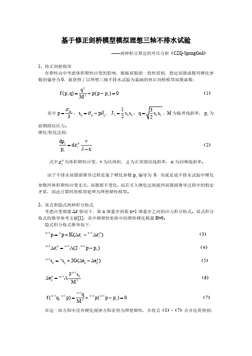
基于修正剑桥模型模拟理想三轴不排水试验——两种积分算法的对比分析(CZQ-SpringGod )1、修正剑桥模型在塑性功中考虑体积塑性应变的影响,根据屈服面一致性原则,假定屈服函数对硬化参数的偏导为0,就获得了以理想三轴不排水试验为基础的修正剑桥模型屈服函数:22(,)()0c q f p q p p p M =+-= (1) 其中3kkp σ=,ij ij ij s p σδ=-,212ij ij J s s =,q =M 为临界线斜率,c p 为前期固结压力。
硬化/软化法则:p c v c dp v d p ελκ=- (2) 式中p v ε为体积塑性应变,v 为比体积,λ为正常固结线斜率,κ为回弹线斜率。
由于不排水屈服面推导过程是基于硬化参数c p 偏导为0,也就是说不排水试验中硬化参数同体积塑性应变无关,屈服面不变化,而若引入硬化法则就同屈服面推导过程中的假定矛盾,因此计算时将模型处理为理想塑性模型。
2、显式和隐式两种积分格式考虑应变增量ε∆驱动下,第n 增量步到第n+1增量步之间的应力积分格式。
显式积分格式的推导参考文献[1],其中弹塑性矩阵中的塑性硬化模量H=0。
隐式积分格式推导如下:11()n n n p v v p p K εε++=+∆-∆ (3) 111(2)n p n n v c p p ε+++∆=Λ⋅- (4) 12()n n p ij ij ij ij s s G e e +=+∆-∆ (5) 1123n ij p n ij s e M ++∆=Λ (6) 111112(,)()0n n n n n c qf q p p p p M +++++=+-= (7)在这一组方程中没有硬化规律方程表明为理想塑性,并将式(3)-(7)合并化简得到:1112112122(2)06()(1)0n n n n v c n n n trial c p p K K p p G q p p p M Mε++++++⎧--∆+⋅Λ⋅-=⎪⎨+-+Λ=⎪⎩ (8) 式中3(2)(2)2n n trial ij ij ij ij q s G e s G e =+∆+∆ 求解(8)式方程组即可得到n+1增量步的各个增量。
Huang_Plasticity1.0_1

塑性力学的特点 塑性力学主要研究材料在出现塑性变形情况下 的变形特征和应力应变关系,是固体力学的一 个重要分支。塑性力学与弹性力学有着密切的 联系。弹性力学中的中有关平衡、变形协调以 及边界条件等概念在塑性力学中同样适用。塑 性力学与弹性力学之间的根本差别在于应力-应 变关系的不同。并且,不同类型材料的塑性变 形规律并不相同,其数学描述也有很大的差异。
材料的流变特性:蠕变
σ ε
ε
t
σ
t 加载与卸载中的蠕变 蠕变积累
§1.1 材料的弹塑性变形
材料的流变特性:应力松弛 关键词: 瞬时变形 elasticity plasticity 蠕变变形 viscosity
ε
σ
t
t
简单的材料力学试验 材料的变形规律,需要通过实验来获得。 最简单的材料力学试验 金属材料: 单轴拉伸/压缩 岩土类材料:常规三轴压缩
σ
全量形式 – 由应变表示应力
σs
ε
−σ s
弹性加载 σ = E (ε − ε 0 ), 当 | ε − ε0 |< εs σ = σ s sign(ε − ε 0 ), 当 | ε − ε 0 | ≥ ε s , (ε − ε 0 )∆ε > 0 塑性加载 当 | σ | = σ s , (ε − ε 0 )∆ε < 0 ∆σ = E ∆ε , 弹性卸载
HOHAI UNIVERSITY
塑 性 力 学 Engineering Plasticity
黄文雄
河海大学力学与材料学院
主要参考书 夏志皋编 “塑性力学”,同济大学出版社,1991 李咏偕、施泽华编 “塑性力学”,水电出版社, 1987 考核 听课、讨论、练习、考试
第一章 绪论
第八章 本构-修正剑桥模型
7.5.1 Elastic properties
常用对数
自然对数
The elastic stiffness is nonlinear and depends on the current stress level.
剑桥模型
7.5.2 Yield criterion
Cam Clay Model Modified Cam Clay Model
(i) Influence of intermediate principal stress on deformation and strength (1)
Stress ratio – strain increment ratio relation Direction of strain increments on octahedral plane
(i) Influence of intermediate principal stress (ii) Stress path dependency of plastic flow (iii) Positive dilatancy during strain hardening (iv) Anisotropy and non-coaxiality (v) Behavior under cyclic loading (vi) Influence of density and confining pressure (vii) Structured soil (viii) Time effect and age effect
' po
pf
qf
M
破坏时
1 p / p 2
' f ' 0
1 k
f
河海大学参考书
考试科目名称
应用生态学 水务规划与管理 现代工程测量 构造地质学 工程地质原理 土壤水动力学 给水排水规划 环境规划评价与管理 物理海洋学 物理化学 河流动力学 现代数据管理技术 随机水文学 高级管理学 桥梁工程 环境水力学 复合材料学 现代水文信息技术 传感器技术与信息处 理 泥沙运动力学 粘性流体动力学 高等水工结构学 线性系统理论 工程项目管理 分布式数据管理技术 软件复用技术 高分子物理 《应用生态学》张金屯主编,科学出版社,2003
-2-
10294 河海大学
2017 年博士研究生招生考试参考范围
考试科 目代码
3036 3037 3038 3039 3040 3041 3042 3044 3045 3053 3056 3058 3059 3063 3065 3066 3070 3082 3083 3085 3086 3087 3089 3094 3096 3097 3100
考试科目名称
政治理论 英语 俄语 日语 德语 法语 数理方程 计算数学 概率论与数理统计 应用统计 管理综合 数理逻辑 环境化学 社会学理论与方法 政治学原理 常微分方程 土地管理综合 马克思主义基本原理 弹性力学 结构力学 岩石力学 电力系统分析 高等土力学
参 考 范 围
《科技哲学概论》丁长青、张雁编著,河海大学出版社,2003.10;《科学技术方法》丁长青编著,河海大学出版社,2003.10; 《自 然辩证法概论》黄顺基主编,教育部社科与思政司编著,高等教育出版社,2004.5 《English Through Reading》W.W.S Bhasker and N.S.Prabhu.Macmillan World Publishing;《研究生英语教程》郑亚南主编,河海大 学出版社 参照相应的硕士专业通用教材 参照相应的硕士专业通用教材 参照相应的硕士专业通用教材 参照相应的硕士专业通用教材 《数学物理方程》陈才生等编,东南大学出版社,2002;或《数学物理方程》陈才生等编,科学出版社,2008。 《矩阵论基础》方保镕主编,清华大学出版社,2004;《数值分析》李庆扬等,清华大学出版社,2007 《概率论与数理统计教程》魏宗舒等编,高等教育出版社 《应用统计学》 (第二版) ,卢冶飞,孙宝忠编著,清华大学出版社,2015 《现代企业管理一变革的观点》黄速建等主编,经济管理出版社;《战略管理》张阳等主编,科学出版社 《面向计算机科学的数理逻辑系统建模与推理》(英文版第 2 版),Michael Huth,Mark Ryan 著,机械工业出版社,2005 年 《环境化学》戴树桂主编,高等教育出版社,2002;《有机污染化学》陆光华编著,河海大学出版社,2011 年 7 月第一版 《社会思想名家》,刘易斯·科塞著,石人译,上海人民出版社,2007 年;《新教伦理与资本主义精神》,马克斯·韦伯著,苏国勋等译, 社会科学文献出版社,2010 年;《社会分工论》,涂尔干著,渠东译,三联书店,2000 年;《规训与惩罚》,福柯著,刘北成等译,三联 书店,2007 年;《社会研究方法》,风笑天著,中国人民大学出版社,2009 年 《政治学概论》孙关宏等主编,复旦大学出版社,2004 年;《政治科学》迈克尔·罗斯金等编,华夏出版社,2001 年 《常微分方程教程》(第二版),丁同仁、李承治编,高等教育出版社 《土地经济学》(第六版)毕宝德主编,中国人民大学出版,2011 年。《土地资源管理学》(第二版)王万茂编著,高等教育出版社,2010 年。 《土地行政管理学》(第二版),曲福田主编,中国农业出版社,2011 年。《土地政策学》(第二版),黄贤金主编,中国农业出版社,2007 年。 《马克思主义基本原理概论》本书编写组,高等教育出版社,2010 年修订版;或有关教材。 《弹性力学》 (上册,第四版)徐芝纶编著,高等教育出版社,2006;《弹性力学》(第 2 版),陈国荣编著,河海大学出版社,2010 《结构静力学》蔡新等编著,河海大学出版社,2004;《结构动力学》(第六章、第七章不考)张子明等编著,河海大学出版社,2004 《岩石力学》徐志英主编,水利水电出版社(第三版),1993 年 6 月第三版 《电力系统分析》(上册),诸俊伟,中国电力出版社; 《电力系统分析》(下册),夏道止,中国电力出版社 《土工原理》,殷宗泽等编著,中国水利水电出版社,2007
经典土力学教材David Muir Wood_ Geotechnical modelling and critical state soil mechanics
Hostun sand Sadek, 2006
ABC120 250
σz
σz
ABC150
distortional probing constant mean stress non-monotonic stress paths stress probe rosettes
-250
ABC90 ABC60 ABC30 C 50 ABC300 150
distortional strain 0.05%: history recalled 1%: history ‘forgotten’
Sadek, 2006
σz 150
stress response envelopes small/medium strain stiffness
B b
C
c 50 a
stress stress
a.
b.
strain
strain
70
yielding of Bothkennar clay: boundaries deduced from inspection of stress:strain response Y1 approximately centred on in situ stress state Y3 reflects natural structure – damaged by any irrecoverable strain - evanescent
Geotechnical modelling and critical state soil mechanics Naples, May 2007
13. Designer models: addition of extra features
固体力学(080102) - 河海大学研究生院
固体力学(080102)学科门类:工学(08) 一级学科:力学(0801)河海大学固体力学学科创建于上世纪五十年代,是我校历史最悠久的学科之一,也是我校力学一级学科最早设立的硕士点。
在著名力学家徐芝伦院士倡导下,本学科坚持基础与应用并重、理论与实践结合,与水利水电工程、土木工程、交通工程、能源工程等交叉渗透,取得了一系列的高水平研究成果。
本学科1993年被国务院学位委员会评为A类,设有力学一级博士后科研流动站,学科队伍与工程力学学科相互交叉,现有教授26人,拥有国家工科力学教学基地、高性能计算中心和力学实验中心,并新建成了国内一流水平的破坏力学实验室,为进一步开展基础理论研究和重大应用研究打下了坚实的基础。
毕业研究生一部分在国内外著名大学继续深造,一部分到高校任教或大型企事业单位从事科研设计工作。
一、培养目标本学科培养力学理论和应用方面的高层次人才,具有严谨求实的科学态度和作风,能够胜任教学、科研或大型工程技术研发和管理工作。
要求掌握数学、力学理论基础以及系统深入的专业知识和有关的工程实践知识;熟练阅读外文资料;对工程问题能正确建立力学-数学模型,并能运用现代基础理论和先进的计算方法及实验技术手段进行研究,具有一定的解决重大工程技术问题的能力。
二、主要研究方向1、材料的力学特性与行为2、计算固体力学3、结构的力学效应测试与健康诊断4、工程结构的断裂与损伤5、多场耦合的力学问题三、学制和学分攻读硕士学位的标准学制为2.5年,学习年限实行弹性学制,最短不低于2年,最长不超过3.5年(非全日制学生可延长1年)。
硕士研究生课程由学位课程、非学位课程和研究环节组成。
硕士研究生课程总学分不少于34学分,其中学位课程不少于20学分,非学位课程不少于9学分,研究环节5学分。
四、课程设置固体力学学科硕士研究生课程设置。
土木工程专业英语词汇集锦
土木工程专业英语词汇(整理版)第一部分必须掌握,第二部分尽量掌握第一部分:1 Finite Element Method 有限单元法2 专业英语 Specialty English3 水利工程 Hydraulic Engineering4 土木工程 Civil Engineering5 地下工程 Underground Engineering6 岩土工程 Geotechnical Engineering7 道路工程 Road (Highway) Engineering8 桥梁工程Bridge Engineering9 隧道工程 Tunnel Engineering10 工程力学 Engineering Mechanics11 交通工程 Traffic Engineering12 港口工程 Port Engineering13 安全性 safety17木结构 timber structure18 砌体结构 masonry structure19 混凝土结构concrete structure20 钢结构 steelstructure21 钢 - 混凝土复合结构 steel and concrete composite structure22 素混凝土 plain concrete23 钢筋混凝土reinforced concrete24 钢筋 rebar25 预应力混凝土 pre-stressed concrete26 静定结构statically determinate structure27 超静定结构 statically indeterminate structure28 桁架结构 truss structure29 空间网架结构 spatial grid structure30 近海工程 offshore engineering31 静力学 statics32运动学kinematics33 动力学dynamics34 简支梁 simply supported beam35 固定支座 fixed bearing36弹性力学 elasticity37 塑性力学 plasticity38 弹塑性力学 elaso-plasticity39 断裂力学 fracture Mechanics40 土力学 soil mechanics41 水力学 hydraulics42 流体力学 fluid mechanics43 固体力学solid mechanics44 集中力 concentrated force45 压力 pressure46 静水压力 hydrostatic pressure47 均布压力 uniform pressure48 体力 body force49 重力 gravity50 线荷载 line load51 弯矩 bending moment52 扭矩 torque53 应力 stress54 应变 stain55 正应力 normal stress56 剪应力 shearing stress57 主应力 principal stress58 变形 deformation59 内力 internal force60 偏移量挠度 deflection61 沉降settlement62 屈曲失稳 buckle63 轴力 axial force64 允许应力 allowable stress65 疲劳分析 fatigue analysis66 梁 beam67 壳 shell68 板 plate69 桥 bridge70 桩 pile71 主动土压力 active earth pressure72 被动土压力 passive earth pressure73 承载力 load-bearing capacity74 水位 water Height75 位移 displacement76 结构力学 structural mechanics77 材料力学 material mechanics78 经纬仪 altometer79 水准仪level80 学科 discipline81 子学科 sub-discipline82 期刊 journal ,periodical83 文献literature84 国际标准刊号ISSN International Standard Serial Number85 国际标准书号ISBN International Standard Book Number86 卷 volume87 期 number88 专著 monograph89 会议论文集 Proceeding90 学位论文 thesis, dissertation91 专利 patent92 档案档案室 archive93 国际学术会议 conference94 导师 advisor95 学位论文答辩 defense of thesis96 博士研究生 doctorate student97 研究生 postgraduate98 工程索引EI Engineering Index99 科学引文索引SCI Science Citation Index100 科学技术会议论文集索引ISTP Index to Science and Tec hnology Proceedings101 题目 title102 摘要 abstract103 全文 full-text104 参考文献 reference105 联络单位、所属单位affiliation106 主题词 Subject107 关键字 keyword108 美国土木工程师协会ASCE American Society of Civil Engineers 109 联邦公路总署FHWA Federal Highway Administration110 国际标准组织ISO International Standard Organization111 解析方法 analytical method112 数值方法 numerical method113 计算 computation114 说明书 instruction115 规范 Specification, Code第二部分:岩土工程专业词汇1.geotechnical engineering 岩土工程2.foundation engineering 基础工程3.soil, earth 土4.soil mechanics 土力学5.cyclic loading 周期荷载6.unloading 卸载7.reloading 再加载8.viscoelastic foundation 粘弹性地基9.viscous damping 粘滞阻尼10.shear modulus 剪切模量11.soil dynamics 土动力学12.stress path 应力路径13.numerical geotechanics 数值岩土力学二.土的分类1.residual soil 残积土 groundwater level 地下水位2.groundwater 地下水 groundwater table 地下水位3.clay minerals 粘土矿物4.secondary minerals 次生矿物ndslides 滑坡6.bore hole columnar section 钻孔柱状图7.engineering geologic investigation 工程地质勘察8.boulder 漂石9.cobble 卵石10.gravel 砂石11.gravelly sand 砾砂12.coarse sand 粗砂13.medium sand 中砂14.fine sand 细砂15.silty sand 粉土16.clayey soil 粘性土17.clay 粘土18.silty clay 粉质粘土19.silt 粉土20.sandy silt 砂质粉土21.clayey silt 粘质粉土22.saturated soil 饱和土23.unsaturated soil 非饱和土24.fill (soil) 填土25.overconsolidated soil 超固结土26.normally consolidated soil 正常固结土27.underconsolidated soil 欠固结土28.zonal soil 区域性土29.soft clay 软粘土30.expansive (swelling) soil 膨胀土31.peat 泥炭32.loess 黄土33.frozen soil 冻土24.degree of saturation 饱和度25.dry unit weight 干重度26.moist unit weight 湿重度45.ISSMGE=International Society for Soil Mechanics and Geotechnical Engineering 国际土力学与岩土工程学会四.渗透性和渗流1.Darcy’s law 达西定律2.piping 管涌3.flowing soil 流土4.sand boiling 砂沸5.flow net 流网6.seepage 渗透(流)7.leakage 渗流8.seepage pressure 渗透压力9.permeability 渗透性10.seepage force 渗透力11.hydraulic gradient 水力梯度12.coefficient of permeability 渗透系数五.地基应力和变形1.soft soil 软土2.(negative) skin friction of driven pile 打入桩(负)摩阻力3.effective stress 有效应力4.total stress 总应力5.field vane shear strength 十字板抗剪强度6.low activity 低活性7.sensitivity 灵敏度8.triaxial test 三轴试验9.foundation design 基础设计10.recompaction 再压缩11.bearing capacity 承载力12.soil mass 土体13.contact stress (pressure)接触应力(压力)14.concentrated load 集中荷载15.a semi-infinite elastic solid 半无限弹性体16.homogeneous 均质17.isotropic 各向同性18.strip footing 条基19.square spread footing 方形独立基础20.underlying soil (stratum ,strata)下卧层(土)21.dead load =sustained load 恒载持续荷载22.live load 活载23.short –term transient load 短期瞬时荷载24.long-term transient load 长期荷载25.reduced load 折算荷载26.settlement 沉降27.deformation 变形28.casing 套管29.dike=dyke 堤(防)30.clay fraction 粘粒粒组31.physical properties 物理性质32.subgrade 路基33.well-graded soil 级配良好土34.poorly-graded soil 级配不良土35.normal stresses 正应力36.shear stresses 剪应力37.principal plane 主平面38.major (intermediate, minor) principal stress 最大(中、最小)主应力39.Mohr-Coulomb failure condition 摩尔-库仑破坏条件40.FEM=finite element method 有限元法41.limit equilibrium method 极限平衡法42.pore water pressure 孔隙水压力43.preconsolidation pressure 先期固结压力44.modulus of compressibility 压缩模量45.coefficent of compressibility 压缩系数pression index 压缩指数47.swelling index 回弹指数48.geostatic stress 自重应力49.additional stress 附加应力50.total stress 总应力51.final settlement 最终沉降52.slip line 滑动线六.基坑开挖与降水1 excavation 开挖(挖方)2 dewatering (基坑)降水3 failure of foundation 基坑失稳4 bracing of foundation pit 基坑围护5 bottom heave=basal heave (基坑)底隆起6 retaining wall 挡土墙7 pore-pressure distribution 孔压分布8 dewatering method 降低地下水位法9 well point system 井点系统(轻型)10 deep well point 深井点11 vacuum well point 真空井点12 braced cuts 支撑围护13 braced excavation 支撑开挖14 braced sheeting 支撑挡板七.深基础--deep foundation1.pile foundation 桩基础1)cast –in-place 灌注桩diving casting cast-in-place pile 沉管灌注桩bored pile 钻孔桩special-shaped cast-in-place pile 机控异型灌注桩piles set into rock 嵌岩灌注桩rammed bulb pile 夯扩桩2)belled pier foundation 钻孔墩基础drilled-pier foundation 钻孔扩底墩under-reamed bored pier3)precast concrete pile 预制混凝土桩4)steel pile 钢桩steel pipe pile 钢管桩steel sheet pile 钢板桩5)prestressed concrete pile 预应力混凝土桩prestressed concrete pipe pile 预应力混凝土管桩2.caisson foundation 沉井(箱)3.diaphragm wall 地下连续墙截水墙4.friction pile 摩擦桩5.end-bearing pile 端承桩6.shaft 竖井;桩身7.wave equation analysis 波动方程分析8.pile caps 承台(桩帽)9.bearing capacity of single pile 单桩承载力teral pile load test 单桩横向载荷试验11.ultimate lateral resistance of single pile 单桩横向极限承载力12.static load test of pile 单桩竖向静荷载试验13.vertical allowable load capacity 单桩竖向容许承载力14.low pile cap 低桩承台15.high-rise pile cap 高桩承台16.vertical ultimate uplift resistance of single pile 单桩抗拔极限承载力17.silent piling 静力压桩18.uplift pile 抗拔桩19.anti-slide pile 抗滑桩20.pile groups 群桩21.efficiency factor of pile groups 群桩效率系数(η)22.efficiency of pile groups 群桩效应23.dynamic pile testing 桩基动测技术24.final set 最后贯入度25.dynamic load test of pile 桩动荷载试验26.pile integrity test 桩的完整性试验27.pile head=butt 桩头28.pile tip=pile point=pile toe 桩端(头)29.pile spacing 桩距30.pile plan 桩位布置图31.arrangement of piles =pile layout 桩的布置32.group action 群桩作用33.end bearing=tip resistance 桩端阻34.skin(side) friction=shaft resistance 桩侧阻35.pile cushion 桩垫36.pile driving(by vibration) (振动)打桩37.pile pulling test 拔桩试验38.pile shoe 桩靴39.pile noise 打桩噪音40.pile rig 打桩机九.固结 consolidation1.Terzzaghi’s consolidation theory 太沙基固结理论2.Barraon’s consolidation theory 巴隆固结理论3.Biot’s consolidation theory 比奥固结理论4.over consolidation ration (OCR)超固结比5.overconsolidation soil 超固结土6.excess pore water pressure 超孔压力7.multi-dimensional consolidation 多维固结8.one-dimensional consolidation 一维固结9.primary consolidation 主固结10.secondary consolidation 次固结11.degree of consolidation 固结度12.consolidation test 固结试验13.consolidation curve 固结曲线14.time factor Tv 时间因子15.coefficient of consolidation 固结系数16.preconsolidation pressure 前期固结压力17.principle of effective stress 有效应力原理18.consolidation under K0 condition K0 固结十.抗剪强度 shear strength1.undrained shear strength 不排水抗剪强度2.residual strength 残余强度3.long-term strength 长期强度4.peak strength 峰值强度5.shear strain rate 剪切应变速率6.dilatation 剪胀7.effective stress approach of shear strength 剪胀抗剪强度有效应力法8.total stress approach of shear strength 抗剪强度总应力法9.Mohr-Coulomb theory 莫尔-库仑理论10.angle of internal friction 内摩擦角11.cohesion 粘聚力12.failure criterion 破坏准则13.vane strength 十字板抗剪强度14.unconfined compression 无侧限抗压强度15.effective stress failure envelop 有效应力破坏包线16.effective stress strength parameter 有效应力强度参数十一.本构模型--constitutive model1.elastic model 弹性模型2.nonlinear elastic model 非线性弹性模型3.elastoplastic model 弹塑性模型4.viscoelastic model 粘弹性模型5.boundary surface model 边界面模型6.Du ncan-Chang model 邓肯-张模型7.rigid plastic model 刚塑性模型8.cap model 盖帽模型9.work softening 加工软化10.work hardening 加工硬化11.Cambridge model 剑桥模型12.ideal elastoplastic model 理想弹塑性模型13.Mohr-Coulomb yield criterion 莫尔-库仑屈服准则14.yield surface 屈服面15.elastic half-space foundation model 弹性半空间地基模型16.elastic modulus 弹性模量17.Winkler foundation model 文克尔地基模型十二.地基承载力--bearing capacity of foundation soil1.punching shear failure 冲剪破坏2.general shear failure 整体剪切破化3.local shear failure 局部剪切破坏4.state of limit equilibrium 极限平衡状态5.critical edge pressure 临塑荷载6.stability of foundation soil 地基稳定性7.ultimate bearing capacity of foundation soil 地基极限承载力8.allowable bearing capacity of foundation soil 地基容许承载力十三.土压力--earth pressure1.active earth pressure 主动土压力2.passive earth pressure 被动土压力3.earth pressure at rest 静止土压力4.Coulomb’s earth pressure theory 库仑土压力理论5.Rankine’s earth pressure theory 朗金土压力理论十四.土坡稳定分析--slope stability analysis1.angle of repose 休止角2.Bishop method 毕肖普法3.safety factor of slope 边坡稳定安全系数4.Fellenius method of slices 费纽伦斯条分法5.Swedish circle method 瑞典圆弧滑动法6.slices method 条分法十五.挡土墙--retaining wall1.stability of retaining wall 挡土墙稳定性2.foundation wall 基础墙3.counter retaining wall 扶壁式挡土墙4.cantilever retaining wall 悬臂式挡土墙5.cantilever sheet pile wall 悬臂式板桩墙6.gravity retaining wall 重力式挡土墙7.anchored plate retaining wall 锚定板挡土墙8.anchored sheet pile wall 锚定板板桩墙十六.板桩结构物--sheet pile structure1.steel sheet pile 钢板桩2.reinforced concrete sheet pile 钢筋混凝土板桩3.steel piles 钢桩4.wooden sheet pile 木板桩5.timber piles 木桩十七.浅基础--shallow foundation1.box foundation 箱型基础2.mat(raft) foundation 片筏基础3.strip foundation 条形基础4.spread footing 扩展基础pensated foundation 补偿性基础6.bearing stratum 持力层7.rigid foundation 刚性基础8.flexible foundation 柔性基础9.embedded depth of foundation 基础埋置深度 foundation pressure 基底附加应力11.structure-foundation-soil interaction analysis 上部结构-基础-地基共同作用分析十八.土的动力性质--dynamic properties of soils1.dynamic strength of soils 动强度2.wave velocity method 波速法3.material damping 材料阻尼4.geometric damping 几何阻尼5.damping ratio 阻尼比6.initial liquefaction 初始液化7.natural period of soil site 地基固有周期8.dynamic shear modulus of soils 动剪切模量9.dynamic ma二十.地基基础抗震1.earthquake engineering 地震工程2.soil dynamics 土动力学3.duration of earthquake 地震持续时间4.earthquake response spectrum 地震反应谱5.earthquake intensity 地震烈度6.earthquake magnitude 震级7.seismic predominant period 地震卓越周期8.maximum acceleration of earthquake 地震最大加速度二十一.室内土工实验1.high pressure consolidation test 高压固结试验2.consolidation under K0 condition K0 固结试验3.falling head permeability 变水头试验4.constant head permeability 常水头渗透试验5.unconsolidated-undrained triaxial test 不固结不排水试验(UU)6.consolidated undrained triaxial test 固结不排水试验(CU)7.consolidated drained triaxial test 固结排水试验(CD)paction test 击实试验9.consolidated quick direct shear test 固结快剪试验10.quick direct shear test 快剪试验11.consolidated drained direct shear test 慢剪试验12.sieve analysis 筛分析13.geotechnical model test 土工模型试验14.centrifugal model test 离心模型试验15.direct shear apparatus 直剪仪16.direct shear test 直剪试验17.direct simple shear test 直接单剪试验18.dynamic triaxial test 三轴试验19.dynamic simple shear 动单剪20.free(resonance)vibration column test 自(共)振柱试验二十二.原位测试1.standard penetration test (SPT)标准贯入试验2.surface wave test (SWT) 表面波试验3.dynamic penetration test(DPT) 动力触探试验4.static cone penetration (SPT) 静力触探试验5.plate loading test 静力荷载试验teral load test of pile 单桩横向载荷试验7.static load test of pile 单桩竖向荷载试验8.cross-hole test 跨孔试验9.screw plate test 螺旋板载荷试验10.pressuremeter test 旁压试验11.light sounding 轻便触探试验12.deep settlement measurement 深层沉降观测13.vane shear test 十字板剪切试验14.field permeability test 现场渗透试验15.in-situ pore water pressure measurement 原位孔隙水压量测16.in-situ soil test 原位试验。
- 1、下载文档前请自行甄别文档内容的完整性,平台不提供额外的编辑、内容补充、找答案等附加服务。
- 2、"仅部分预览"的文档,不可在线预览部分如存在完整性等问题,可反馈申请退款(可完整预览的文档不适用该条件!)。
- 3、如文档侵犯您的权益,请联系客服反馈,我们会尽快为您处理(人工客服工作时间:9:00-18:30)。
p
p
p
σ1
σ1
σ1
σ2
Cone type
σ3
σ2
Cap type
σ3 σ2
2 yield surface
σ3
(3)hardening law f (σ ) = k
ij
σ
k2 k1
After yield, k changes, How does k change? Which factor causes k change? k increases — hardening k decreases — softening k constant — theoretical
σ1
Variation of yield surface
if f > k , k changes, yield surface moves
σ
k2 k1
q
σ2
f =k
σ3
σ1
ε
p
σ2
σ3
Loading and unloading
Current stress state — on yield surface, A new stress increment is applied. * unloading
σ1
Failure surface —— locus of the points in stress space which represent failure
Failure criterion
σ2
σ3
Trasca criterion
= kf 2 σ σ 2 σ σ 1 σ σ 3 σ1 σ 2 σ σ 1 σ σ 3 k f 2 k f 2 k f 3 k f 3 k f 1 kf = 0 2 2 2 2 2 2
g (σ δε = δλ σ
p ij
ij
)
g (σ
ij
)
δε
δε 3p
p
2
ij
Strain space is overlapped with stress space. Plastic strain increment is perpendicular to plastic potential surface
σ
k1 k2
hardening
ε
softening
k = F (H ) f (σ ij ) = F (H ) f (σ ij , H ) = 0
ε
σ
H — hardening parameter, a physical variant which causes k change For a given value of H, yield surface is defined.
σ
σ ij
σ ij
δσ ij
σ ij
δε p
σ ij
δW p
ε
δσ ij
f
σ1
σ ij = σ ij σ + δσ ij
ij
in loading unloading ,
δW = σ ijδε > 0
p
(σ
ij
σ ij )δε ijp + δσ ijδε ijp > 0
p ij
σ ij
α
δε ijp
f f
g= f
σ2 ε2
σ2 ε2
Non-associated flue rule
p ij
σ 1 ε1
σ ij
σ ij
α
δε ijp
f
(σ
ij
σ ij )δε ijp < 0 σ ij
σ2 ε2
α ≥ 90°
is perpendicular to yield surface f if not,
α ≥ 90°
ε σ1 1 σ ij
σ 1 ε1
σ ij
δε ijp
α
σ ij
4. Elasto-plastic model
ε =εe +ε p ε e —— recoverable strain, elastic ε p —— irrecoverable strain, plastic
σ
{ε } = {ε e }+ {ε p }
Plastic strain
ε
p
εe
ε
。failure criterion, yield criterion 。hardening law 。flue rule
σ
π
plane
σ1
Mohr-Coulunb Trasca Mises
σ1
σ2
σ3
σ2
σ3
σ1 σ3
2
1 2 1 q= 2 q=
=
σ1 +σ3
2
sin + c cos
σ 2 = σ 3 + b(σ 1 σ 3 )
(σ 1 σ 2 )2 + (σ 2 σ 3 )2 + (σ 1 σ 3 )2 (σ 1 σ 3 )2 (1 b )2 + b2 (σ 1 σ 3 )2 + (σ 1 σ 3 )2
σ1 σ 3
Hexagonal column Saturated soil, undrained
τ
c
σ 1 σ 2 = 2c
kf = c
σ1
σ
σ2
σ3
Mises criterion
q = kf
q= 1 2
σ1
(σ 1 σ 2 )2 + (σ 2 σ 3 )2 + (σ 3 σ 1 )2
Circular column surface Extensive Mises criterion
(1)failure criterion
σ < kf σ = kf
elastic failure
f
σ
kf
simple stress state
f f
(σ ) = k complicate stress state (σ ) —— failure function
ij ij
ε
variables are stress components
[
]
σ2
—— second deviator stress invariant 1 J2 = q I1 = 3 p 3
σ3
Circular cone surface
Cambridge university q = Mp
q M
q = M (p + pr )
q= 1 2
1 3
(σ 1 σ 2 )2 + (σ 2 σ 3 )2 + (σ 3 σ 1 )2
df = f dσ ij < 0 σ ij
σ1
dσ ij
n
α
2 vectors multiply elastic
σ2 σ1
n
α > 90 °
* loading
f df = dσ ij > 0 σ ij
α
dσ ij
α < 90 °
plastic
* neutral loading
f df = dσ ij = 0 σ ij
σ2
σ 1 ε1
p ij
If σ on yield surface,
ij
δσ ijδε > 0
(σ
σ ij )δε ijp > δσ ijδε ijp ij
(σ
ij
σ ij )δε ijp ≥ 0
σ ij
σ ij
α
δε ijp
f
α ≤ 90°
σ2 ε2
derivation
*All the points which represent the stress σ ij must be on the other side of the plane perpendicular to δε ijp yield surface f must be convex. if concave * δε
σ
k
( ) ( )
ε
τ =τ f τ <τf
p
theoretical material, yield = failure geotechnical material, yield ≠ failure
τ
τ f = σ tan + c
τ =0
σ
εv
p
εv
Yield surface
f (σ ij ) — yield function, corresponding to yield surface in stress space yield surface — locus of the points in stress space which reach yield
δε
— plastic strain increment Direction of δε p determines each component of the plastic strain increment. Flue rule gives direction of δε p
p
δε1p
δε
p
Conceive a plastic potential function
dε vp deijp = dε ijp δ ij 3
1, (i = j ) δ ij = 0, (i ≠ j )
4.
ε p = ∫ dε p = ∫ dε ijp dε ijp
5.
H = f ε vp , ε sp