麻省理工信号课程教程24
美国MIT信号与系统课程的基本结构

MIT 2009 年秋季学期信号与系统课程教学日程表 Wednesday / Recitation 备注 教学内容 Thursday / Lecture 教学内容 L1 : Signals and Systems L3 : Feedback, Cycles and Modes L5 : Feedback Control Schemes L7 : Laplace Transforms and Z Friday / Recitation 教学内容 R2 : Difference Equations R4 : Feedback, Cycles and Modes R6 : Feedback Control Schemes R8 : Laplace Transforms and Z
பைடு நூலகம்
由 S. Mahajan 和 D. Freeman 于 2009 年编著的《离 。教 学 内 容 涵 盖 了 散时间 信 号 与 系 统: 算 子 法 》 Oppenheim著作的全部主要内容。 此外, 还包括补充
表1 日期 / 课型 周次 1 2 3 4 5 6 7 8 9 10 11 12 13 14 15 Tuesday / Lecture 教学内容 ( Registration Day) L2 : DT Systems L4 : Feedback and Position Control L6 : CT Systems,Difference Eqs. L8 : CT Operator Representations ( For Columbus Day) L11 : Frequency sponse ReHW1 due HW2 due HW3 due EX4 HW5 due HW6 due EX7 HW8 due HW9 due EX10 HW11 due HW12 due EX13
《信号与系统》课程教学改革与实践

秀. 埘 嗍 @ 2 3忍 ・ 6
维普资讯
中国 现代瓣 装 各
过程 。这样组织课程 内容还能避免与数学课程相关知识的重 复, 也体现 了信号与系统 的工程特性而淡化数学复杂性。
在授课过程 中尽量理 论联系实际,将信号的调制解 调理 论的讲解与交通广播 系统 的实际联 系起来;将抽样定理与电 话通信联系起来;将信号滤波与非正弦周期信 号的分解与合 成的实验现象联系起来 。理论联系实际可 以调动学生的学习 积极性 ,也能够 加学 生对基本理论 的理解,还 能够培养学生
的4 主 干 课 程 之 ~ 。 门
多与时间少的矛盾 。另一方面,学生对经过复杂 的数学运算 和推导得到的理论结果缺乏实际应用的认识 ,不能进一步体
会求解结果 即是信 号的应用 l 。 2 ] 其次, 现有教材的例题习题不适合 电气及其 自动化与 自动 化专业教学, 现有教材中的例题、系统基本上是与通信与信息
作者 简介 : 阚江明 ,讲的微分算子模型, 电路中时 将
域的微积分关系转化为简单乘除运算关系。在离散系统的时 域分析的讲授过程中, 同样引入差分算子简化差分方程的求解
・ 金项 目:2 5 北京林 业大学校 级教 改项 目 ( 0 — 基 0 年 0 2 0 5
维普资讯
2 8 第 期 总 6期 0 年 9 (第 7 ) 0
中 现代毂有 备 国 装
《 信号与系统》 课程 教学改革与 实践 书
阚 江 明 燕 飞 张 军 国
北京林业大 学 北京 1 0 8 0 03
摘 要 :( 号与 系统》是 电子信 息类专业 的核 心技 术基础课 ,提 高教学质量和教 学效果对培 养电子信 息类合格人 才有重 《 信
“ 信号与系统”的教学 目的是让学生掌握信号和线性系 统分析的基本理论、基本原理和方法,能够在后续课程 的学
麻省理工大学 数字通讯原理 课程课件MIT6_450F09_slide25
11
ˆ(f ) −1 u �
2T
� � �
� �� � � �� � �� � �� ��
1 2T
3 2T
�� �� � �� �� �
−1 2T
� �� ���� � �� ��� � �� �� �� �
ˆ s (f )
�� � ��� �� � �
���� �
1 2T
�
0
�� �
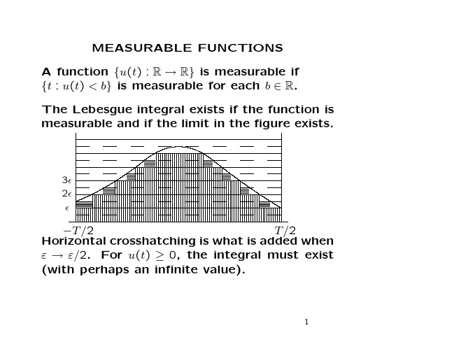
measurable and if the limit in the figure exists.
3
2
−T /2 T /2 Horizontal crosshatching is what is added when
ε → ε/2. For u(t) ≥ 0, the integral must exist
s(t) = u(kT ) sinc − k .
T k t u(t) = l.i.m. vm(kT ) sinc −k T m,k s(kT ) = u(kT ) =
�� �
m
�
�
�
�
�
�
e2πimt/T
vm(kT )
�
(Aliasing)
�
t
vm(kT ) sinc s(t) = − k .
� �� �� � �� � � �
0
Theorem: Let u ˆ(f ) be L2, and satisfy
|f |→∞
ˆ(f )|f |1+ε = 0 lim u
for ε > 0.
Then u ˆ(f ) is L1, and the inverse transform u(t) is continuous and bounded. For T > 0, the � t + k ) is sampling approx. s(t) = k u(kT ) sinc( T bounded and continuous. ˆ s(f ) satisfies � m u ˆ(f + ) rect[f T ]. ˆ s(f ) = l.i.m. T m
信号分与处理-第1课(涂然)

概述
基本内容
信号处理 指通过对信号的加工和变换,把一个信号变换 成另 个信号的过程; 成另一个信号的过程; 也可以更直观的理解为——为了特定的目的, 通过一定手段改造信号
概述
基本内容
强调 这门课不是数学课 虽然有大 的公式推导,但是最终目的是应用 虽然有大量的公式推导,但是最终目的是应用 它们解决工程实际问题 ——这是官方的说法 在我看来,如果这都不算是数学,那数学还能 是什么?
课程安排
课程定位
目标 了解信号分析、处理的基本概念 掌握信号在各种变换域下的分析方法及特性 掌握信号的数字分析基础方法 适当了解现代信号分析、处理的基本内容 提升解决相关问题的能力
课程安排
课程定位
难易程度 以基础知识为主,绝对不讲得太难太偏
fi /
人数 爱提意见
还得努力的
学习好的
课程安排
课程定位
信号分析与处理
涂 然
Mar. 2015, Xiamen
College of Mechanical Engineering and Automation Huaqiao University E-mail: Turan@
自我介绍
自我介绍
涂然 男 1985年生于重庆 涂然,男, 受教育经历
各种分类
信号分类
辨析 通常,仅在有限时间区间内不为0的信号是能 信号 如脉冲信号等 量信号——如脉冲信号等
现实中大多数信号都是这种持续时间有限信号
各种分类
信号分类
辨析 而一般幅度有限的周期信号、随机信号则属于 功率信号
电压噪声
各种分类
信号分类
辨析 重要的一点:对于一个信号 可以既不是能 信号, 不是功率信号 可以既不是能量信号,也不是功率信号 但不能既是能量信号, 又是功率信号
信号ppt课件

按所具有的时间特性划分:
确定信号和随机信号; 连续信号和离散信号;
周期信号和非周其信号; 能量信号和功率信号;
一维信号和多维信号; 因果信号与反因果信号;
实信号与复信号;
左边信号与右边信号。
第 11 页
1. 确定信号和随机信号
•确定性信号:可用确定的时间函数表示的信号:f(t)
第 26 页
三.几种典型确定性信号
1.指数信号 2.正弦信号
3.复指数信号 4. 抽样信号(Sampling Signal)
本课程讨论确定性信号
先连续,后离散;先周期,后非周期。
第 27 页
指数信号 f (t ) K e t
0 直流(常数)
0
f t
0
0 指数衰减, 0 指数增长
-1.5
或写为:
1,
2,
1.5,
f
(k )
2,
0,
1,
0,
k 1 k 0 k 1 k2 k3 k 4 其他k
f(k)= {…,0,1,2,-1.5,2,0,1,0,…} ↑
k=0 对应某序号k的序列值称为第k个样点的“样值”。
第 15 页
模拟信号、抽样信号、数字信号
•模拟信号: 时间
第一章 信号与系统
学习的主要内容:
认识本课程领域的一些名词、术语 学习信号运算规律、熟悉表达式与波形的对应关系 理解冲激信号的特性 了解本课程研究范围、学习目标 初步了解本课程用到的主要方法和手段
第1页
第一章 信号与系统
§1.1 绪论
什么是信号?什么是系统?为什么把这两 个概念连在一起?
信号的概念 系统的概念
MIT(麻省理工)信号与系统讲义-lecture2

Fall 2003 Lecture #2
9 September 2003 1) Some examples of systems 2) System properties and examples a) Causality b) Linearity c) Time invariance
11
CAUSAL OR NONCAUSAL
depends on causal
noncausal
depends on future
depends on future
noncausal
depends on
causal
12
TIME-INVARIANCE (TI)
Informally, a system is time-invariant (TI) if its behavior does not depend on what time it is. • Mathematically (in DT): A system x[n] → y[n] is TI if for any input x[n] and any time shift n0, If x[n] →y[n] then x[n -n0] →y[n -n0] •Similarly for a CT time-invariant system, If x(t) →y(t) then x(t -to) →y(t -to) .
• This system detects changes in signal slope
7
Observations
1)A very rich class of systems (but by no means all systems of interest to us) are described by differential and difference equations. 2)Such an equation, by itself, does not completely describe the input-output behavior of a system: we need auxiliary conditions (initial conditions, boundary conditions). 3)In some cases the system of interest has time as the natural independent variable and is causal. However, that is not always the case. 4)Very different physical systems may have very similar mathematical descriptions.
麻省理工数字通信课程2
12
CHAPTER 2. DISCRETE-TIME AND CONTINUOUS-TIME AWGN CHANNELS
The two parameters W and SNR turn out to characterize the channel completely for digital communications purposes; the absolute scale of P and N0 and the location of the band B do not affect the model in any essential way. In particular, as we will show in Chapter 3, the capacity of any such channel in bits per second is C[b/s] = W log2 (1 + SNR) b/s. If a particular digital communication scheme transmits a continuous bit stream over such a channel at rate R b/s, then the spectral efficiency of the scheme is said to be ρ = R/W (b/s)/Hz (read as “bits per second per Hertz”). The Shannon limit on spectral efficiency is therefore C[(b/s)/Hz] = log2 (1 + SNR) (b/s)/Hz; i.e., reliable transmission is possible when ρ < C[(b/s)/Hz] , but not when ρ > C[(b/s)/Hz] .
MIT 公开课程 信号与系统 Lecture 2
6.003:Signals and SystemsDiscrete-Time SystemsFebruary4,2010Discrete-Time SystemsWe start with discrete-time(DT)systems because they•are conceptually simpler than continuous-time systems•illustrate same important modes of thinking as continuous-time•are increasingly important(digital electronics and computation)From Samples to SignalsLumping all of the(possibly infinite)samples into a single object—the signal—simplifies its manipulation.This lumping is an abstraction that is analogous to•representing coordinates in three-space as points•representing lists of numbers as vectors in linear algebra•creating an object in PythonLet Y=R X.Which of the following is/are true:1.y[n]=x[n]for all n2.y[n+1]=x[n]for all n3.y[n]=x[n+1]for all n4.y[n−1]=x[n]for all n5.none of the aboveOperator ApproachApplies your existing expertise with polynomials to understand block diagrams,and thereby understand systems.Example: AccumulatorThese systems are equivalent in the sense that if each is initially atrest, they will produce identical outputs from the same input.(1 −R ) Y 1 = X 1⇔ ?Y 2 =(1+ R + R 2+ R 3+ ···) X 2Proof: Assume X 2 = X 1:Y 2 =(1+ R+ R 2 + R 3 + ···) X 2 =(1+ R + R 2 + R 3 + ···) X 1 = (1+ R + R 2 + R 3 + ···)(1 −R ) Y 1= ((1 + R + R 2 + R 3 + ···) −(R + R 2 + R 3 + ···)) Y 1 = Y 1It follows that Y 2 = Y 1.It also follows that (1 −R) and (1 + R + R 2 + R 3 + ···) are reciprocals .Example: AccumulatorThe reciprocal of 1−R can also be evaluated using synthetic division.1+R +R 2 +R 3 + ···1 −R 11 −RRR −R 2R 2R 2 −R 3R 3R 3 −R 4···Therefore1=1+ R + R 2 + R 3 + R 4 + ··· 1 −RAnalysis of Cyclic Systems:Geometric GrowthIf traversing the cycle decreases or increases the magnitude of the signal,then the fundamental mode will decay or grow,respectively.If the response decays toward zero,then we say that it converges. Otherwise,we it diverges.M IT OpenCourseWare6.003 Signals and SystemsSpring 2010For information about citing these materials or our Terms of Use, visit: /terms.。
MIT 信号与系统 Lecture 19
April 15, 2010
Homework 11 will not collected or graded. Solutions will be posted. Closed book: 3 pages of notes (8 1 2 × 11 inches; front and back). Designed as 1-hour exam; two hours to complete. Review sessions during open office hours. April 15, 2010
ω s-plane z -plane
H (e j Ω ) = H (z )|z =e j Ω
σ
|H (jω )|
H (ej Ω )
1
0
ω
−π
0
πΩ
Check Yourself
A system H (z ) = 1 − az has the following pole-zero diagram. z−a z -plane
x[7]
Number of multiples increases as N 2 .
8 × 8 = 64 multiplications
FFT
Divide into two 4-point series (divide and conquer). Even-numbered entries ⎡ ⎤ ⎡ 0 0 a0 W4 W 4 ⎢a ⎥ ⎢W0 W1 ⎢ 1⎥ ⎢ 4 4 ⎢ ⎥=⎢ 0 2 ⎣ a2 ⎦ ⎣ W4 W4 0 3 a3 W4 W4 Odd-numbered entries ⎡ ⎤ ⎡ 0 0 W4 W4 b0 ⎢b ⎥ ⎢W0 W1 ⎢ 1⎥ ⎢ 4 4 ⎢ ⎥=⎢ 0 2 ⎣ b2 ⎦ ⎣ W 4 W 4 0 3 W4 W4 b3 in x[n]:
MIT课程设置
美国MIT EECS系本科生课程设置简介清华大学郑君里于歆杰研究美国MIT(麻省理工学院)EECS(电气工程与计算机科学)系的课程安排,可以给我们一些启示,供我国同类系科教学改革参考。
国内已有一些文章对此给出介绍[1-3]。
但是由于该校课程门类很多,与国内教学计划的形式差别较大,往往不容易看清楚核心问题。
本文将MIT课程计划(2005—2006)列成一些表格,以突出要点,从而便于和我国情况进行比较。
首先,给出课程分类及学分,见表1。
表1课程类型划分、大致门数和学分MIT学分统计原则与我国情况不同。
每门课程要计入讲授、实验、复习自学(课外)三部分时间。
例如,电路与电子学为4+2+9=15学分(其中,每周讲课4学时,实验2学时,课后复习9学时),大致相当于我国的5~6学分(每周5~6学时,课内)。
因此,372学分对应我国约372/3=124学分(或稍多至148.8)。
我们关心电气工程与计算机科学本科的主要基础课程设置,下面着重讨论表1中的EECS必修课和限选课程两部分共10门课程的情况,略去其他内容的分析。
表2给出全系必修课。
表2 EECS全体必修课程对EECS系全体学生划分为3个学习(与研究)方向,见表3。
表33个方向及其与我国情况对比与此同时,将全部课程划分为7个工程领域,见表4,每个学习方向的学生按照各自方向规定之原则从7个领域中选取不同课程做组合。
表47个工程领域涉及的主要课程下面给出3个方向限选课程的指导原则,并举出可能构成的选课实例,见表5,这里的5门限选课加上表2的5门必修课以及表1中限选数学1门和限选实验1门共计12门课,大约在2—3年级学完。
将此处结果与我国各系2—3年级主修的10多门课程对照,即可看出二者的区别与共同之处。
表53个方向的选课原则(从7个领域的许多课程中选5门)课程设置特点及其与我国情况比较:(1)统一、坚实的系级平台核心课:表2中的课程是本学科基础知识的精华,全系学生必修。
- 1、下载文档前请自行甄别文档内容的完整性,平台不提供额外的编辑、内容补充、找答案等附加服务。
- 2、"仅部分预览"的文档,不可在线预览部分如存在完整性等问题,可反馈申请退款(可完整预览的文档不适用该条件!)。
- 3、如文档侵犯您的权益,请联系客服反馈,我们会尽快为您处理(人工客服工作时间:9:00-18:30)。
Amplitude, Phase, and Frequency Modulation
There are many ways to embed a “message” in a carrier. Here are three. Amplitude Modulation (AM): Phase Modulation (PM): Frequency Modulation (FM): y1 (t) = x(t) cos(ωc t) y2 (t) = cos(ωc t + kx(t)) � � �t y3 (t) = cos ωc t + k −∞ x(τ )dτ
Find the Fourier transform of a PM signal. x(t) = sin(ωm t)
y (t) = cos(ωc t + mx(t)) = cos(ωc t + m sin(ωm t))
= cos(ωc t) cos(m sin(ωm t))) − sin(ωc t) sin(m sin(ωm t)))
Find the Fourier transform of a PM signal. x(t) = sin(ωm t)
y (t) = cos(ωc t + mx(t)) = cos(ωc t + m sin(ωm t))
= cos(ωc t) cos(m sin(ωm t))) − sin(ωc t) sin(m sin(ωm t)))
x1(t)
cos x2(t) cos x3(t) cos
3t 2t 1t
z1(t)
z2(t)
z(t) cos
ct
LPF
y(t)
z3(t)
Superheterodyne Receiver
Edwin Howard Armstrong invented the superheterodyne receiver, which made broadcast AM practical.
Find the Fourier transform of a PM signal. x(t) = sin(ωm t)
y (t) = cos(ωc t + mx(t)) = cos(ωc t + m sin(ωm t))
= cos(ωc t) cos(m sin(ωm t))) − sin(ωc t) sin(m sin(ωm t)))
2π
, therefore cos(m sin(ω t)) is periodic in T . x(t) is periodic in T = ω m m
cos(m sin(ωm t)) 1 0 −1 m = 30 |ak | 0 10 20 30 40 50 60 k t
Phase/Frequency Modulation
2π
, therefore cos(m sin(ω t)) is periodic in T . x(t) is periodic in T = ω m m
cos(m sin(ωm t)) 1 0 −1 m=1 |ak | 0 10 20 30 40 50 60 k t
Phase/Frequency Modulation
Amplitude Modulation
Amplitude modulation can be used to match audio frequencies to
radio frequencies. It allows parallel transmission of multiple channels.
Find the Fourier transform of a PM signal. x(t) = sin(ωm t)
y (t) = cos(ωc t + mx(t)) = cos(ωc t + m sin(ωm t))
= cos(ωc t) cos(m sin(ωm t))) − sin(ωc t) sin(m sin(ωm t)))
• bandwidth?
Frequency Modulation
Early investigators thought that narrowband FM could have arbitrar ily narrow bandwidth, allowing more channels than AM. Wrong! � � � t x(τ )dτ y3 (t) = cos ωc t + k −∞ � � � t � � t � = cos(ωc t) × cos k x(τ )dτ − sin(ωc t) × sin k x(τ )dτ
Phase/Frequency Modulation
Find the Fourier transform of a PM signal. x(t) = sin(ωm t)
y (t) = cos(ωc t + mx(t)) = cos(ωc t + m sin(ωm t))
= cos(ωc t) cos(m sin(ωm t))) − sin(ωc t) sin(m sin(ωm t)))
Find the Fourier transform of a PM signal. x(t) = sin(ωm t)
y (t) = cos(ωc t + mx(t)) = cos(ωc t + m sin(ωm t))
= cos(ωc t) cos(m sin(ωm t))) − sin(ωc t) sin(m sin(ωm t)))
Edwin Howard Armstrong also invented and patented the “regenerative” (positive feedback) circuit for amplifying radio signals (while he was a junior at Columbia University). He also in vented wide-band FM.
Find the Fourier transform of a PM signal. x(t) = sin(ωm t)
y (t) = cos(ωc t + mx(t)) = cos(ωc t + m sin(ωm t))
= cos(ωc t) cos(m sin(ωm t))) − sin(ωc t) sin(m sin(ωm t)))
2π
, therefore cos(m sin(ω t)) is periodic in T . x(t) is periodic in T = ω m m
cos(m sin(ωm t)) 1 0 −1 m=0 |ak | 0 10 20 30 40 50 60 k t
Phase/Frequency Modulation
2π
, therefore cos(m sin(ω t)) is periodic in T . x(t) is periodic in T = ω m m
cos(m sin(ωm t)) 1 0 −1 m = 10 |ak |
0 10 20 30 40 50 k 60
t
Phase/Frequency Modulation
6.003: Signals and Systems
Modulation
May 6, 2010
Communications Systems
Signals are not always well matched to the media through which we wish to transmit them. signal audio video internet applications telephone, radio, phonograph, CD, cell phone, MP3 television, cinema, HDTV, DVD coax, twisted pair, cable TV, DSL, optical fiber, E/M
2π
, therefore cos(m sin(ω t)) is periodic in T . x(t) is periodic in T = ω m m
cos(m sin(ωm t)) 1 0 −1 m=5 |ak | 0 10 20 30 40 50 60 k t
Phase/Frequency Modulation
2π
, therefore cos(m sin(ω t)) is periodic in T . x(t) is periodic in T = ω m m
Frequency Modulation
Compare AM to FM for x(t) = cos(ωm t). AM: y1 (t) = (cos(ωm t) + 1.1) cos(ωc t)
t
FM: y3 (t) = cos(ωc t + m sin(ωm t))
t
Advantages of FM: • constant power • no need to transmit carrier (unless DC important)
Find the Fourier transform of a PM signal. x(t) = sin(ωm t)
y (t) = cos(ωc t + mx(t)) = cos(ωc t + m sin(ωm t))
= cos(ωc t) cos(m sin(ωm t))) − sin(ωc t) sin(m sin(ωm t)))
−∞ −∞
If k → 0 then � � t � x(τ )dτ → 1 cos k −∞ � � t � � t sin k x(τ )dτ → k x(τ )dτ −∞ −∞ � � t � y3 (t) ≈ cos(ωc t) − sin(ωc t) × k x(τ )dτ