Stabilized Kuramoto-Sivashinsky equation A useful model for secondary instabilities and rel
KitAlysis

KitAlysis™ Suzuki-Miyaura Cross-CouplingReaction Screening KitCatalog Number KITALYSIS-SMStore at Room TemperatureTECHNICAL BULLETINProduct DescriptionThe KitAlysis™ Suzuki-Miyaura Cross-Coupling Reaction Screening Kit enables chemists to quickly and efficiently screen conditions for the coupling of aryl halides with organoboronic acids.Quick identification of optimal conditions allows faster scale-up of the desired synthetic transformation. All required chemicals come pre-weighed for ease of use.Each Suzuki-Miyaura Cross-Coupling Reaction Screening Kit contains 4 individual screening sets. Each screening set has components to run 24 unique Suzuki-Miyaura reactions:∙10 μmol (het)aryl halide (user supplied)∙15–20 μmol (het)aryl boronate (user supplied)∙ 1 μmol catalyst per vial (1:1 Pd:Ligand); 6 in this system∙30 μmol base (1.5 M K3PO4)∙0.1 M solvent concentration (DMAc, Toluene, n-butanol, and THF) Access /kitalysis for detailed step-by-step Protocols and Scale-up Guide. The Protocols include an introductory video, instructions for the Labware, and work-up/internal standard addition procedures.A downloadable spreadsheet for stock solution recipes for each screening set is available from the step-by-step Protocol.The spreadsheet provides:∙Calculations for substrate recipes based on the molecular weight of user supplied substrates∙Quick directions for experienced users∙Print button allows you to take experimental recipes to the lab∙Contains all experimental information, which can easily be saved as a pdf file and appended toelectronic laboratory notebooksScreening Kit Components∙Four screening sets individually sealed under nitrogen in mylar bags. Each bag includes 24 glass vials loaded with stir bars and pre-weighedcatalysts (1 μmol), see Figures 1 and 2∙Ampule boxes containing degassed, anhydrous liquids:4 ⨯ 2 mL Toluene4 ⨯ 2 mL THF4 ⨯ 2 mL n-Butanol4 ⨯ 2 mL DMAc4 ⨯ 2 mL aq. 1.5 M K3PO4∙Biphenyl Internal Standard (15.4 mg)∙ 4 New KitAlysis 24-Well Reaction BlockReplacement Films∙ 4 substrate stock solution vials with stir bars2 Figure 2. CatalystsFigure 3.Positions of CatalystsSuggested Equipment (Not Provided)∙ 96-well plate for automated HPLC analysis(Catalog Number Z688711)∙ 96-well plate cap mat for automated HPLC analysis(Catalog Number C1111)∙ 10–100 μL pipette (Catalog Number Z683809) ∙ 2–200 μL pipette tip refill (Catalog NumberZ640220)∙ 100–1,000 μL pipette (Catalog Number Z683825) ∙ 50–1,000 μL pipette tip refill (Catalog NumberZ640247)∙ 2-inch needles for ease of ampule solventextraction (Catalog Number Z192570)∙ 1 mL syringe for accurate solvent volume extractionfrom ampule (Catalog Number Z230723)Specially designed KitAlysis Labware allows screening set up in a hood without the use of a glove box.∙ KitAlysis Benchtop Inertion Box (Catalog NumberZ742064)∙ KitAlysis 24-well Reaction Block and Screwdriver(Catalog Number Z742107)∙ KitAlysis 24-well Reaction Block and Intertion BoxStarter Set (Catalog Number Z742108)Instructions for the Labware can be accessed in the Articles section of the website product display page for the kit.Precautions and DisclaimerThis product is for R&D use only, not for drug,household, or other uses. Please consult the Safety Data Sheet for information regarding hazards and safe handling practices.Storage/StabilityStore the kit at room temperature.KitAlysis is a trademark of Sigma-Aldrich Co. LLC.DR,MAM 08/16-2©2016 Sigma-Aldrich Co. LLC. All rights reserved. SIGMA-ALDRICH is a trademark of Sigma-Aldrich Co. LLC, registered in the US and other countries. Aldrich brand products are sold through Sigma-Aldrich, Inc. Purchaser must determine the suitability of the product(s) for theirparticular use. Additional terms and conditions may apply. Please see product information on the Sigma-Aldrich website at and/or on the reverse side of the invoice or packing slip.。
【国家自然科学基金】_hausdorff_基金支持热词逐年推荐_【万方软件创新助手】_20140730
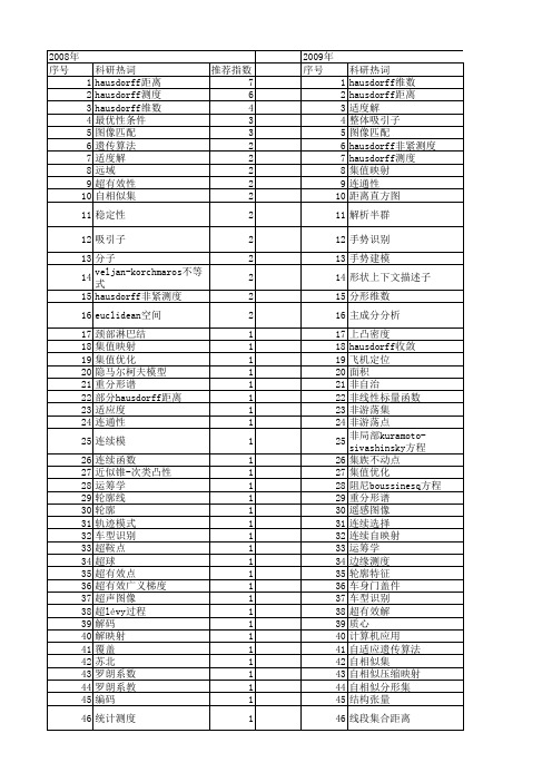
科研热词 推荐指数 hausdorff距离 7 hausdorff测度 6 hausdorff维数 4 最优性条件 3 图像匹配 3 遗传算法 2 适度解 2 远域 2 超有效性 2 自相似集 2 稳定性 2 吸引子 2 分子 2 veljan-korchmaros不等式 2 hausdorff非紧测度 2 euclidean空间 2 颈部淋巴结 1 集值映射 1 集值优化 1 隐马尔柯夫模型 1 重分形谱 1 部分hausdorff距离 1 适应度 1 连通性 1 连续模 1 连续函数 1 近似锥-次类凸性 1 运筹学 1 轮廓线 1 轮廓 1 轨迹模式 1 车型识别 1 超鞍点 1 超球 1 超有效点 1 超有效广义梯度 1 超声图像 1 超lévy过程 1 解码 1 解映射 1 覆盖 1 苏北 1 罗朗系数 1 罗朗系教 1 编码 1 统计测度 1 统计收敛 1 线段hausdorff距离 1 紧支撑 1 稳定过程 1 积分微分适度解 1 碎片拼合 1
免疫遗传算法 体积 仿射运动分类器 人脸识别 人脸特征定位 人脸定位 交互式图像分割 主动形状模型 临界指数 严有效解 严有效 不动点 下半连续性 上自相似集 上半连续性 上半连续函数 上凸密度 sierpinski地毯 sierpinski 垫片 scott拓扑 rectifiable集 lévy过程 k-s假设检验 icp算法 hilbert方体 hausdorff跟踪 hausdorff拓扑 hausdorff 测度 hausdorff hausdoff 维数 harris角点 gabor小波 fuzzy测度 fpga fourier变换 contourlet变换 contingent上图切导数 cantor集 c0-半群 brown运动 box雏数 ban54 55 56 57 58 59 60 61 62 63 64 65 66 67 68 69 70 71 72 73 74 75 76 77 78 79 80 81 82 83 84 85 86 87 88 89 90 91 92 93 94 95 96 97 98 99 100 101 102 103 104 105 106
【国家自然科学基金】_连串反应_基金支持热词逐年推荐_【万方软件创新助手】_20140803
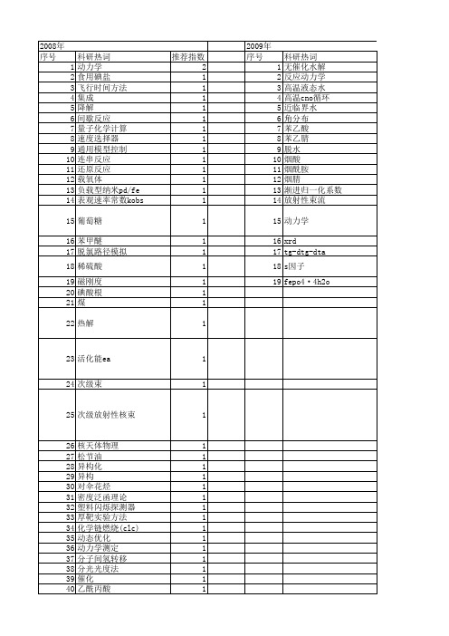
科研热词 动力学 食用碘盐 飞行时间方法 集成 降解 间歇反应 量子化学计算 速度选择器 通用模型控制 连串反应 还原反应 载氧体 负载型纳米pd/fe 表观速率常数kobs 葡萄糖 苯甲醚 脱氯路径模拟 稀硫酸 磁刚度 碘酸根 煤 热解 活化能ea 次级束 次级放射性核束 核天体物理 松节油 异构化 异构 对伞花烃 密度泛函理论 塑料闪烁探测器 厚靶实验方法 化学链燃烧(clc) 动态优化 动力学测定 分子间氢转移 分光光度法 催化 乙酰丙酸 中间体 不确定参数 caso4
2011年 序号 1 2 3 4 5 6 7 8 9 10 11 12
2011年 科研热词 非线性拟合 非等温动力学 重结晶 迪开石 近临界水 过程强化 聚丙烯腈 研究进展 热分解 混合 无催化水解 反应动力学 推荐指数 1 1 1 1 1 1 1 1 1 1 1 1
2012年 序号 1 2 3 4 5 6 7 8 9 10 11 12 13 14 15 16 17 18 19 20 21 22 23 24 25 26 27
2013年 序号 1 2 3 4 5 6 7 8 9 10 11 12 13 14 15 16 17 18
科研热词 推荐指数 硝解 2 反应动力学 2 sex 2 n2o5 2 hmx 2 dadn 2 酶学过程 1 自碱化 1 硝基苯 1 甲苯氯化 1 性能分析 1 对氨基苯酚 1 反硝化 1 反应精馏 1 双功能催化剂 1 催化加氢 1 侧反应器-精馏塔集成系统 1 亚硝氮积累 1
【国家自然科学基金】_多项式混沌_基金支持热词逐年推荐_【万方软件创新助手】_20140730

推荐指数 2 1 1 1 1 1 1 1 1 1 1 1 1 1 1 1 1 1 1 1 1 1 1 1 1 1 1 1 1 1 1 1 1 1 1 1 1 1 1 1 1 1 1 1 1 1
2011年 序号 1 2 3 4 5 6 7 8 9 10 11 12 13 14 15 16 17 18 19 20 21 22 23 24 25 26 27 28 29 30 31 32 33 34 35 36 37 38 39 40
2011年 科研热词 chebyshev多项式 混沌映射 实数域 多项式混沌 公钥加密 非线性微分反馈控制 随机最优控制 随机对流扩散方程 随机响应面方法 阶跃函数 遗传算法 蔡氏电路 自适应混沌多项式 自适应机制 网格多涡卷混沌吸引子 绝对节点坐标 电路实现 混沌多项式 混沌 柔性多体系统 方腔流动 数值模拟 投影寻踪回归 扰动 待定系数法 异宿轨道 密钥 安全性 多重网格 地震动 参数随机振荡电路系统 加密 光滑型chua系统 交通流量预测 不确定性 shilnikov定理 lorenz legendre karhunen-loève展开 duffing振子 推荐指数 3 2 2 2 2 1 1 1 1 1 1 1 1 1 1 1 1 1 1 1 1 1 1 1 1 1 1 1 1 1 1 1 1 1 1 1 1 1 1 1
2012年 序号 1 2 3 4 5 6 7 8 9 10 11 12 13 14 15 16 17 18 19 20 21 22 23 24 25 26 27 28 29 30 31 32 33 34 35 36 37 38
科研热词 推荐指数 预处理器 2 随机过程数值仿真 2 随机对流扩散方程 1 随机场 1 软测量 1 身份认证 1 蒙特卡洛方法 1 脉冲控制 1 结构可靠度 1 稀疏性 1 矢量基 1 混沌级数 1 混沌现象 1 混沌映射 1 混沌控制 1 混合核 1 最小二乘支持向量机 1 无单元galerkin方法 1 方腔流动 1 数值模拟 1 数值仿真精度实验与分析 1 平移多项式基函数 1 平方和算法 1 层递响应面法 1 层递响应面 1 小波动态自适应网格 1 密钥协商 1 多项式混沌 1 多项式浑沌展开 1 多项式模型 1 向量 1 半群特性 1 动态自适应小波方法 1 不确定性 1 rsa算法 1 kuramoto-sivashinsky方程 1 krylov子空间 1 chebyshev多项式 1
Nonlocal Kuramoto-Sivashinsky方程近似惯性流形的构造
No. 9
N no a K rmooSv sisy方 程 o lcl ua t—iahnk
近 似 惯 性 流 形 的 构 造
罗 宏
( 川师 范 大 学 四 数 学 与 软 件科 学 学 院 , 都 成 606 ) 10 6
摘
要 : 究 了 N n cl ua o —i sisy方程 解的 长时 间行 为 , 用压 缩 映像 原理 , 研 o l a K rm t Sv h k o o a n 利 构
造 了方 程 的 近 似 惯 性 流 形 , 得 到 了近 似 惯 性 流 形 逼 近 方 程 全 局 吸 引 予 的 阶 数 估 计 。 并
关 键 词 : o l a K rm t S ahnk N n cl ua o —i sisy方程 ; o o v 近似 惯性 流 形 ; 缩 映像 原 理 ;阶数 估计 压
保证惯 性 流形存 在性 的条 件十 分苛刻 ( 比如谱 间 隙条 件 ) ,因此 许 多 重要 的无穷 维 动 力 系统 的惯 性 流形
的存 在性 仍未解 决 , 于是 自然想 到用 一种 近似 的 、 光滑 的 、 比较 容 易求解 的流 形去逼 近整 体 吸 引子 和惯 性
收 稿 E 期 :0 0— 5—2 t 21 0 4
Kur m o o- v s n ky Eq to a t Si a hi s ua i n
L UO n Ho g
( o ee f t mac n otaeSine Sc unN r a U i r t, hnd 0 6 hn ) C lg h tsadSf r c c , i a om l nv syC egu6 6 ,C ia l o Ma e i w e h ei 1 0
Integrating Factor Methods as Exponential Integrators

Integrating Factor Methods asExponential IntegratorsBorislav V.MinchevDepartment of Mathematical Science,NTNU,7491Trondheim,NorwayBorko.Minchev@ii.uib.noAbstract.Recently a lot of effort has been placed in the constructionand implementation of a class of methods called exponential integrators.These methods are preferable when one has to deal with stiffand highlyoscillatory semilinear problems,which often arise after spatial discretiza-tion of Partial Differential Equations(PDEs).The main idea behind themethods is to use the exponential and some closely related functionsinside the numerical scheme.In this note we show that the integratingfactor methods,introduced by Lawson in1967,are also examples of expo-nential integrators with very special structure for the related exponentialfunctions.In order to prove this relation,we use the approach based onbi-coloured rooted trees and B-series.We also show under what condi-tions every bi-coloured rooted tree can be express as a linear combinationof standard non-coloured rooted trees.1IntroductionRealistic models of many physical processes require effective numer-ical solvers for a special class of partial differential equations,which after semidiscretization in space can be written in the following formu =Lu+N(u(t)),u(t0)=u0,(1.1)where u:R→R d,L∈R d×d,N:R d→R d and d is a discretiza-tion parameter equal to the number of spatial grid points.Several interesting problems can be brought to this form.Examples are Allen-Cahn,Burgers,Cahn-Hilliard,Kuramoto-Sivashinsky,Navier-Stokes,Swift-Hohenberg,nonlinear Scr¨o dinger equations.Typically the linear part of the problem will be stiffand the nonlinear part will be nonstiff.Many numerical integrators have been developed to overcome the phenomenon of stiffness.Exponential integrators was introduced in the early sixties as an alternative approach for solving2stiffsystems.The main idea behind these methods is to integrate exactly the linear part of the problem and then use an appropriate approximation of the nonlinear part.Thus the exponential function, and functions which are closely related to the exponential function, appear in the format of the method.This was the reason why,until recently,these methods have not been regarded as practical.The latest achievements in thefield of computing approximations to the matrix exponential,have provided a new interest in the construction and implementation of exponential integrators[2,3,6,7,9].The main requirements imposed on the functions,which appear in the format of an exponential integrator are,to be analytic,map the spectrum of L into a bounded region in C and can be computed exactly or up to arbitrary high order cheaply.Suppose that,for all l∈N andλ∈R,the operatorsφ[l](λ):R d×d→R d×d satisfy the above conditions and can be expanded in the formφ[l](λ)(hL)= j≥0φ[l]j(λ)(hL)j.Theφ[l]functions,which are used in practice are associated with the so called Exponential Time Differencing methods[3,4,10,11], and can be written explicitly asφ[l](λ)(hL)=(λhL)−l eλhL−l−1 k=0(λhL)k k! .(1.2)If h represents the stepsize and U i denotes the internal stage ap-proximation of the exact solution for i=1,2,...,s then the compu-tations performed in step number n of an exponential Runge–Kutta (RK)method are related by the equationsU i=sj=1s l=1α[l]ijφ[l](c i)(hL)hN(U j)+e c i hL u n−1,u n=sj=1s l=1β[l]jφ[l](1)(hL)hN(U j)+e hL u n−1,(1.3)whereα[l]ij andβ[l]j are the parameters of the method and the vector c=(c1,c2...,c s)T is the abscissae vector.Ifα[l]ij=0for all j≥i3 the method is explicit and implicit otherwise.Alternatively the com-putations performed in step number n can be represented in a more Runge–Kutta type formulation as followscα[1]α[2]···α[s],β[1]Tβ[2]T···β[s]Twhere each element in row number i of the matrixα[l]is multiplied byφ[l](c i)(hL)and each element in the vectorβ[l]T is multiplied by φ[l](1)(hL).The resulting matrices are then added in a component by component sense.Other important class of methods which are also used for solving the semilinear problem(1.1)are the Integrating Factor(IF)methods. The idea behind these methods goes back to the work of Lawson [8].He proposes to ameliorate the effect of the stifflinear part of equation(1.1)by using change of variables(also known as Lawson transformation),v(t)=e−tL u(t).The initial value problem(1.1)written in the new variable isv (t)=e−tL N(e tL v(t))v(t0)=v0,(1.4) where v0=e−t0L u0.The approach now is to apply an arbitrary s-stage Runge–Kutta method to the transformed equation(1.4)and then to transform the result back into the original variable.Thus,a method which satisfy just the nonstifforder conditions will not suffer from sever order reduction,when it is applied to stiffproblems.The aim of this paper is to show that the IF methods are ex-amples of exponential RK methods with special choices for theφ[l] functions and the parametersα[l]andβ[l]T.We also prove that in this special case the nonstifforder theory for the exponential RK methods reduces to the classical Runge–Kutta order theory,which explains why the IF methods exhibit the expected order.The paper is organized as follows:we briefly survey the nonstifforder theory for the exponential RK methods in Section2.Next,in Section3,we define the structure the matricesα[l]and the vectors β[l]T as well as the form of the functionsφ[l],which correspond to the IF methods.Finally,in Section4,we conclude with several remarks and questions of future interest.42Nonstifforder conditionsThe nonstifforder theory for the exponential RK methods was first constructed in [4]and later developed in [11].Here we follow the approach suggested in [9].It is based on bi-coloured rooted trees and B-series.For those not familiar with these concepts we suggest the monographs [1,5]for a complete treatment.Let 2T ∗denote the set of all bi-coloured (black and white)rooted trees with the requirement that the valency of the white nodes is always one.This correspods to the fact that the first term on the right hand side of (1.1)is linear.Let ∅represents the empty set which remains if the root of the one node tree or is removed.The order of the tree τ∈2T ∗is defined as the number of vertices in the tree,and it is denoted by |τ|.The density γof the tree is defined as the product over all vertices of the order of the subtree rooted at that vertex.An exponential Runge–Kutta method with elementary weight function a :2T ∗→R ,has nonstifforder p ,if for all τ∈2T ∗,such that |τ|≤p ,a (τ)=1/γ(τ).In order to give a practical representation of the elementary weight function a of the numerical solution,it is convenient to in-troduce some notations.Let for l =0,1,...and k =1,...,m the s ×smatrix φ[k ]l (c )=diag φ[k ]l (c 1),...,φ[k ]l (c s ) and C =diag(c 1,...,c s ).DefineA [l ]=s k =1φ[k ]l (c )α[k ],b [l ]T =s k =1φ[k ]l (1)β[k ]T ,C [l ]=1(l +1)!C l +1.(2.1)The elementary weight function a of the numerical solution can be computed using the following non-recursive rule:–Attach b [j ]Tto the root black node.–Attach A [j ]to all remaining nonterminal black nodes.–Attach A [j ]e to all terminal black nodes.–Attach C [j ]e to all terminal white nodes.–Attach I to all remaining white nodes.5 The value j is the number of white nodes directly below the corre-sponding node,I is the s×s identity matrix and e=(1,...,1)T. Now for each tree multiply from the root to the leaf as in the case for Runge–Kutta methods,then multiply these expressions in a compo-nent by component sense.3IF methods as a special caseApplying a standard s-stage Runge–Kutta method to the trans-formed equation(1.4)and then transforming back the result into the original variable,leads us to the followingφ[l]functionsφ[l](λ)(hL)=e(λ−c l)hL.(3.1) Every IF method can be represented in the form(1.3)withφ[l]func-tions given by(3.1)and with a special choice of the coefficient ma-tricesα[l]and the coefficient vectorsβ[l]T.This choice reduces the set of all order conditions to a set,which consists only of the order conditions corresponding to the black trees.To proof of this fact we need the following lemma.Lemma1.Let t∈R\{0,−1,−2,...},then for j=0,1,2,...jk=0(−1)k k!(j−k)!1(k+t)=1.t(t+1)···(t+j)Proof.The proof of this statement is by induction on j.The following theorem defines the structure of the matricesα[l] and the vectorsβ[l]T for the IF methods.With this structure of the coefficients,to achieve certain nonstifforder,it is sufficient to satisfy only the black trees.This implies that the transformed differential equation(1.4)is solved using a Runge–Kutta method.Theorem1.Let all the non-zero coefficients of an exponential Runge–Kutta method(1.3),withφ[l]functions given by(3.1)be located in column number l of the matrixα[l]and in position number l of the vectorβ[l]T for l=1,2,...,s.The method has nonstifforder p iffall order conditions corresponding to the black trees are satisfied.6Proof.It follows directly that if the exponential Runge–Kutta method has nonstifforder p then all order conditions corresponding to the black trees are satisfied.Let us assume that all the order conditions corresponding to the black trees are satisfied.We need to prove that all the remaining order conditions are also satisfied.From the defi-nition of theφ[l]functions(3.1),it follows that for j=0,1,2,...,φ[l]j(1)=(1−c l)jj!,φ[l]j(c)=1j!diag((c1−c l)j,...,(c s−c l)j).(3.2)Since all order conditions corresponding to the black trees involve only the coefficients A[0],b[0]T and c,we need to express every other order condition in terms of these coefficients.Having in mind the special structure of the matricesα[l]and the vectorsβ[l]T,after sub-stituting(3.2)into(2.1),we obtain for j=1,2,...,A[j]=jk=0(−1)k k!(j−k)!C[0]j−k A[0]C[0]k,b[j]T=jk=0(−1)k k!(j−k)!b[0]T C[0]k.(3.3)From the fact that all order conditions corresponding to the black trees are satisfied,it follows that A[0],b[0]T and c form a Runge–Kutta method.Therefore,C[0]e=A[0]e,C[0]ζ=(A[0]e)ζ,C[0]kζ=(A[0]e)...(A[0]e)ζ,(3.4)whereζis an arbitrary vector and the multiplications between the elements in the brackets are in a component by component sense.Now,we are in a position to define a procedure which transforms every coloured treeτinto a linear combination of black trees of order at most|τ|.Each treeτcan be decomposed asτ=(τb,τj,τt), whereτb is a coloured tree on the bottom with less number of white nodes thanτ;τj is tall white tree with j≥1white nodes andτt is black tree on the top.First applying formula(3.3)and then(3.4), for the order condition corresponding to a treeτ,we obtain the following three representations in terms of black trees or trees with7less white vertices.If τt =∅then τreduces toτ==If τb =∅then τreduces toτ==δ0+···+δ+···+δ,where δk =(−1)k k !(j −k )!for k =0,1,2,...,j .In the general case when τ{t,b }=∅,then τcan be representedas τ==δ+···+δk+···+δj (3.5)For each of the trees in the linear combination we apply the same procedure.Thus,after a finite number of steps all the trees in the combination will be black.From (2.1)it is clear that the order of every single black tree cannot exceed the order of coloured tree.To complete the proof we need to show that a (τ)=1/γ(τ)for all coloured trees τ,where |τ|≤p .We prove this by induction on the number of steps θin the transformation process.Let θ=1.Every coloured tree τhas representation τ= jk =0δk τk ,where all τk areblack trees.If γ(τt )=x 1|τt |x 2then a (τk )=1γ(τk )=1x 1(|τt |+k )x 2and by Lemma 1for t =|τt |it follows thata (τ)=j k =0(−1)k k !(j −k )!a (τk )=jk =0(−1)k k !(j −k )!1x 1(|τt |+k )x 2=1x 1|τt |(|τt |+1)···(|τt |+j )x 2=1γ(τ).Assume that a (τ)=1/γ(τ)for all coloured trees τwith θsteps in the transformation process.Let τbe a tree with θ+1steps in the transformation process.From (3.5)it follows that τ= j k =0δk τk ,8whereτk are coloured trees withθsteps in the transformation pro-cess and hence a(τk)=1/γ(τk).Ifγ(τt)=x1|τt|x2then a(τk)=1γ(τk)=1x1(|τt|+k)x2and by Lemma1for t=|τt|it again follows thata(τ)=1/γ(τ).4ConclusionsWe have shown that the IF methods are examples of exponential Runge–Kutta methods with special structure of the coefficients ma-trices and the relatedφ[l]functions.We have also proven that,in this special case,the nonstifforder theory for the exponential RK meth-ods reduces to the classical Runge–Kutta order theory.This explains why the IF methods exhibit the expected order.Other examples of theφ[l]functions,rather than(1.2)and(3.1),arise from the frame-work of Lie group methods see[9].The question how tofind the best set ofφ[l]functions is open and needs further investigation. References1.J.C.Butcher,Numerical methods for ordinary differential equations,John Wi-ley&Sons,2003.2.M.Calvo and C.Palencia,A class of explicit multistep exponential integrators forsemilinear problems,preprint,2005.3.P.M.Cox and P.C.Matthews,Exponential time differencing for stiffsystems,J.Comput.Phys.176(2002),430–455.4. A.Friedli,Verallgemeinerte Runge–Kutta verfahren zur l¨o esung steifer differen-tialgleichungssysteme,Lect.Notes Math.631(1978).5. E.Hairer,C.Lubich,and G.Wanner,Geometric numerical integration,Springer,2003,Number31in Springer Series in Computational Mathematics.6.M.Hochbruck and A.Osterman,Explicit exponential Runge–Kutta methods forsemilinear parabolic problems,Submitted to SIAM J.Numer.Anal.,2004.7.Exponential Runge–Kutta methods for parabolic problems,To appear in Appl.Nu-mer.Math.,2004.wson,Generalized Runge–Kutta processes for stable systems with large Lips-chitz constants,SIAM J.Numer.Anal.4(1969),372–390.9. B.Minchev,Exponential integrators for semilinear problems,Ph.D.thesis,Univer-sity of Bergen,2004.10.S.Nørsett,An A-stable modification of the Adams-Bashforth methods,Lect.NotesMath.109(1969),214–219.11.K.Strehmel and R.Weiner,B-convergence results for linearly implicit one stepmethods,BIT27(1987),264–281.。
【国家自然科学基金】_精确孤立波解_基金支持热词逐年推荐_【万方软件创新助手】_20140801
2009年 序号 1 2 3 4 5 6 7 8 9 10 11 12 13 14 15 16 17 18 19 20 21 22
科研热词 辅助方程 函数变换 非线性差分微分方程 孤立波解 孤立波 周期波 非线性弯曲波 行波解 联立薛定谔方程组 有限挠度 扭结波 尖波 孤子 周期波解 周期 分支理论 光滑波 riecati方程 klein-gordon方程 jacobi椭圆函数展开 hamilton系统 ablowitz-方程
推荐指数 3 3 2 2 2 2 1 1 1 1 1 1 1 1 1 1 1 1 1 1 1 1
2010年 序号 1 2 3 4 5 6 7 8 9 10 11 12 13 14 15 16 17 18 19 20 21 22 23 24 25 26 27 28 29
科研热词 推荐指数 孤立波 3 精确解 2 孤波解 2 周期波解 2 周期波 2 非线性扭转波方程 1 非线性差分微分方程 1 解的叠加公式 1 紧解 1 椭圆函数 1 指数函数展开法 1 广义(2+1)维bkp方程 1 孤立波解 1 周期尖波 1 周期孤立波解 1 双曲函数正切法 1 双周期孤立波解 1 双周期双孤立波解 1 光滑孤立波 1 光滑周期波 1 三角函数型辅助方程 1 kdv方程 1 jacobi椭圆函数 1 hirota方法 1 camassa-holm-kp方程 1 bbm系统 1 (n+1)维双sine-gordon方程 1 (3+1)维k-p方程 1 (2+1)-维流体力学型系统 1
2013年 序号 1 2 3 4 5 6 7 8 9 10 11 12 13 14 15 16 17 18 19 20 21 22 23 24 25 26 27
科研热词 推荐指数 动力系统理论 2 光滑孤立波 2 光滑周期波 2 齐次平衡法 1 精确孤立波解 1 符号计算 1 稳定性 1 离散mkdv方程 1 相图 1 条件稳定性 1 有界解 1 改进的tanh函数法 1 扭波解 1 微扰解 1 广义非线性耗散超弹性杆波动方程1 广义二维bbm方程 1 广义(n+1)维boussinesq方程 1 孤立波解 1 孤波解 1 周期波解 1 双扭结单孤子 1 动力系统分支理论 1 分支理论 1 1 schr(o)dinger-kdv方程 1 mkdv方程 1 lyapunov特征指数 1
摩托尔斯丁机器人模型3B的用户指南说明书
3B SCIENTIFIC ® PHYSICS1Motore Stirling G 1002594Istruzioni per l'uso10/23 ALF/UD1 Volano con marcaturaper determinare il numero di giri2 Unità motore-generatorecon puleggia a due stadi 3 Interruttore 4 Lampadina5 Jack di sicurezza da 4mm6 Bruciatore ad alcol7 Prese di misura dellatemperatura 18 Pistone di compressione 9 Attacco del tubo contappo per la misurazione della pressione10 Prese di misura dellatemperatura 2 11 Pistone di lavoro 12 Asta filettata M3(collegata al pistone di lavoro)1. Norme di sicurezzaRiempire con attenzione il bruciatore ad alcol con alcol da ardere, in modo tale che non fuoriesca.Non riempire il bruciatore ad alcol se lostoppino sta ancora bruciando o se nelle vicinanze è presente un’altra fiamma aperta. Dopo l’uso chiudere immediatamente ilflacone di alcol.Non avvicinare le mani alla fiamma aperta. Attenzione! Spegnere la fiamma solo con ilcoperchio fissato.Il motore Stirling si riscalda durante il funzionamento con fiamma aperta.Non toccare il cilindro di compressionedurante e al termine del funzionamento del motore Stirling.Lasciare raffreddare il motore prima dirimuoverlo.2. DescrizioneIl motore Stirling permette l’analisi qualitativa e quantitativa del ciclo di Stirling. Può essere utilizzato in tre modalità diverse: motore termico, pompa di calore o macchina frigorifera.Il cilindro e il pistone di compressione sono realizzati in vetro resistente alle alte temperature; il cilindro di lavoro, il volano e le protezioni del cambio sono invece in vetro acrilico. In questo modo è possibile osservare molto bene i singoli movimenti in qualsiasi momento. Gli alberi a gomiti hanno cuscinetti a sfera e sono realizzati in acciaio temprato. Le bielle sono di plasticaresistente all’usura.L’unità motore-generatore incorporata, dotata di puleggia a due stadi consente di trasformare l’energia meccanica generata in energia elettrica. Con possibilità di commutazione per l’azionamento di una lampada incorporata o di carichi esterni, oppure per alimentare energia elettrica per il funzionamento in qualità di pompa di calore o macchina frigorifera.Fissando il filo in dotazione all'asta filettata del pistone di lavoro, è possibile misurarne la corsa.23. Dati tecniciUnità motore-generatore: max. 12 V CC Puleggia a due stadi: 30 mm Ø, 19 mm Ø Pistone di lavoro: 25 mm Ø Corsa pistone di lavoro: 24 mm Variazione del volume:24 mm 325mm 12cm 2Volume minimo: 32 cm³ Volume massimo: 44 cm³Potenza del motore Stirling: ca. 1 WDimensioni: ca. 300x220x160 mm³ Peso: ca. 1,65 kg4. Schema di funzionamentoIl ciclo Stirling ideale avviene in 4 fasi:1a fase: fase di espansione: cambiamento distato isotermico, l’aria si espande a temperatura costante2a fase: cambiamento di stato isocorico, l’ariasi raf fredda a volume costante nel rigeneratore3a fase: fase di compressione: cambiamentodi stato isotermico, l’aria viene compressa in modo isotermico4a fase: cambiamento di stato isocorico, l’ariaviene di nuovo riscaldata alla temperatura origina ria nel rigeneratoreNel motore Stirling, questo processo ideale è realizzato solo in maniera approssimativa, perché i quattro tempi si sovrappongono. Il gas passa da caldo a freddo già durante la fase di espansione e durante la fase di compressione l’aria non si trova ancora tutta nella parte fredda del motore.Fig. 1 Schema di funzionamento(A: Pistone di compressione, B: Pistone di lavoro)5. Utilizzo5.1 Il motore Stirling come motore termico Riempire il bruciatore ad alcool, inserirlonell’incavo della piastra di base, estrarre svitando lo stoppino di circa 1-2 mm e accenderlo.Portare i pistoni di compressione nellaposizioni più arretrata e dopo un breve periodo di riscaldamento (da 1 a 2 minuti circa) mettere in movimento il volano con una leggera pressione in senso orario (sguardo rivolto verso l'unità motore-generatore) (vedere fig. 2).Se necessario, impostare la tensione dellacinghia di trasmissione spostando l'unità motore-generatore. Accendere la lampadina spostandol'interruttore nella posizione “sopra”.In alternativa collegare il carico esternotramite le prese da 4 mm e mettere in funzione con l’interruttore in posizione "sotto".Numero di giri senza carico: ca. 1000 giri/min Numero di giri congeneratore come carico: ca. 650 giri/min Tensione generatore: ca. 6 V CC Scarto di pressione: +250 hPa/-150 hPa5.2 Il motore Stirling come pompa di calore omacchina frigoriferaDotazione supplementare necessaria:1 Alimentatore CC, 0 - 20 V, 0 - 5 A @ 230 V1003312oppure1 Alimentatore CC, 0 - 20 V, 0 - 5 A @ 115 V1003311Termometro digitale 1002794 Inserire i sensori di temperatura nelle presedi misura della temperatura e collegarli ad un misuratore (vedere fig. 3).Collegare la sorgente di corrente continuatramite le prese da 4 mm.Impostare al massimo 12 V e azionare ilmotore di Stirling con l'interruttore in posizione "sotto".Osservare l’aumento o la diminuzione ditemperatura.In modalità di funzionamento macchina frigorifera il volano ruota in senso orario (sguardo rivolto verso l'unità motore-generatore), in modalità pompa di calore in senso antiorario.Per cambiare la modalità difunzionamentoinvertire la polarità dei cavi di collegamento.3Scarto di pressione: +250 hPa/-150 hPa Tensione motore: 9 V Numero di giri: 600 giri/minDifferenza di temperatura (riferita a 21° C): Macchina frigorifera: -4 K (serbatoio: +6 K) Pompa di calore: +13 K (serbatoio: -1 K)5.3 Registrazione del diagramma pressione-volume del motore Stirling come pompa di caloreDotazione supplementare necessaria:1 Alimentatore CC, 0 - 20 V, 0 - 5 A @ 230 V1003312oppure1 Alimentatore CC, 0 - 20 V, 0 - 5 A @ 115 V10033111 Portasensori per motore Stirling G 1008500 1 Sensore di pressione relativa ±1000 hPa 1021533 1 Rilevatore di corsa FW 10215342 Cavos del sensore 1021514 1 Data logger 1 SoftwareUlteriori informazioni sulla misurazione digitale sono disponibili sul sito web del prodotto, nel webshop 3B.Fissare il portasensori alla piastra di base delmotore Stirling.Nel portasensori, montare il sensore dipressione relativa in basso e il rilevatore di corsa in alto in modo tale che il lato stampato sia rivolto verso l’alto.Collegare l’attacco del tubo “+” del sensore di pressione relativa e l’attacco tubo sul cilindro di lavoro del motore Stirling per mezzo del tubo flessibile fornito in dotazione con il portasensori (1008500).Avvitare il dado cieco fissato al filo (compreso nella dotazione del portasensori) sull’asta filettata del pistone di lavoro, passare il filo intorno alla puleggia del rilevatore di corsa e appendere la molla ad elica all’asta filettata. (Per una descrizione dettagliata relativa al montaggio dei sensori sul portasensori vedere le istruzioni per l’uso del portasensori 1008500.)Collegare il sensore di pressione relativa e il rilevatore di corsa al data logger.Collegare la sorgente di corrente continua tramite le prese da 4 mm.Impostare al massimo 12 V e azionare il motore di Stirling con l'interruttore in posizione "sotto".Avviare il software e registrare il diagramma pressione-volume.Fig.2Il motore Stirling come motore termico3B Scientific GmbH Ludwig-Erhard-Straße 20 20459 Amburgo • Germania • Con riserva di modifiche tecniche © Copyright 2023 3B Scientific GmbHFig. 3 Il motore Stirling come pompa di calore o macchina frigoriferaFig. 4 Registrazione del diagramma pressione-volume。
PREPARATION OF MEDICAL HARD CAPSULE
专利名称:PREPARATION OF MEDICAL HARD CAPSULE 发明人:ARAUME KIYOSHI,MUTOYASUAKI,NISHIYAMA YUICHI,CHIBA TORU申请号:JP14562689申请日:19890608公开号:JPH039755A公开日:19910117专利内容由知识产权出版社提供摘要:PURPOSE:To efficiently prepare a medical hard capsule whose wall part has a uniform thickness by coating a pin with an aqueous solution of hydroxypropyl methyl cellulose having structural viscosity in its flow characteristics and drying the coated pin to mold the prototype of the capsule and releasing said product to cut the same into a predetermined length. CONSTITUTION:The concn. of an aqueous solution of hydroxypropyl methyl cellulose is 15-25wt.% and the viscosity thereof at 40 deg.C is3,000-15,000cps and the ratio of the viscosity measured after standing for 30min at 40 deg.C and the viscosity measured at a shear rate of 1.5sec<-1> immediately after sufficient stirring is 130% or more. A pin having the shape corresponding to the respective body and cap of a medical hard capsule is immersed in the aqueous solution of hydroxypropyl methyl cellulose to be drawn up and the aqueous solution is applied to the pin and dried to mold the prototype of the capsule. The prototype is released from the pin to be cut into a predetermined length and the obtained body and cap are engaged with each other to make it possible to obtain a medical hard capsule whose wall part has a uniform thickness.申请人:SHIN ETSU CHEM CO LTD更多信息请下载全文后查看。
Engagement device in automatic transmission
专利名称:Engagement device in automatictransmission发明人:Seitoku Kubo,Koujiro Kuramochi,Tatsuo Kyushima申请号:US06/190034申请日:19800923公开号:US04380179A公开日:19830419专利内容由知识产权出版社提供摘要:In an automatic transmission including sun gears, ring gears and a carrier for rotatably supporting a pinion on a shaft, the pinion being adapted to mesh with the sun gear and the ring gear; the improvements comprising a hub extending radially outside of the ring gear and having a friction surface in part of the outer peripheral wall thereof and external spline teeth provided in the other part of the outer peripheral wall, the hub being attached to the carrier; a friction element adapted to engage a cylindrical outer race fitted on internal spline-teeth of a transmission housing and the friction face of the hub; a plurality of first friction plates axially, slidably fitted on the external spline teeth of the hub; and a plurality of second friction plates axially, slidably fitted on the internal spline-teeth of the transmission housing, the first and second friction plates disposed one after another.申请人:TOYOTA JIDOSHA KOGYO KABUSHIKI KAISHA代理机构:Finnegan, Henderson, Farabow, Garrett & Dunner更多信息请下载全文后查看。
- 1、下载文档前请自行甄别文档内容的完整性,平台不提供额外的编辑、内容补充、找答案等附加服务。
- 2、"仅部分预览"的文档,不可在线预览部分如存在完整性等问题,可反馈申请退款(可完整预览的文档不适用该条件!)。
- 3、如文档侵犯您的权益,请联系客服反馈,我们会尽快为您处理(人工客服工作时间:9:00-18:30)。
a r X i v :0809.1964v 1 [n l i n .P S ] 11 S e p 2008APS/123-QEDThe Stabilized Kuramoto-Sivashinsky Equation:A Useful Model For Secondary Instabilities and Related Dynamics of Experimental One-Dimensional Cellular FlowsP.Brunet 1,2∗1KTH Mechanics -SE -10044Stockholm,Sweden2School of Mathematics,University of Bristol,University Walk,Bristol BS81TW,United Kingdom(Dated:September 11,2008)We report numerical simulations of one-dimensional cellular solutions of the stabilized Kuramoto-Sivashinsky (SKS)equation.This equation offers a range of generic behavior in pattern-forming instabilities of moving interfaces,like a host of secondary instabilities or transition toward disorder.We compare some of these collective behaviors to those observed in experiments.In particular destabilization scenarios of bifurcated states are studied in a spatially semi-extended situation,which is common in realistic patterns,but was barely explored so far.PACS numbers:47.54.-r,47.20.MaAn interface that is driven out-of-equilibrium fre-quently develops a patterned structure,characterized by a spatially periodic array of identical cells.This pattern can in turn show a set of various secondary instabilities,until a possible transition to disorder [1].Such a scenario has been encountered in various experiments,such as di-rectional solidification [2,3],directional viscous finger-ing [4,5,6],Taylor-Dean flow [7],a locally heated thin layer of liquid [8]or an array of falling liquid columns [9,10,11,12,13].Coullet and Iooss [14]have proposed a generic model,based on broken symmetries that predicts ten secondary instabilities from a primary static periodic cellular struc-ture.This model reproduced successfully many features of secondary modes associated to broken symmetries on the primary pattern,for instance parity-broken (PB)do-mains of drifting cells [15]or vacillating-breathing (VB)mode leading to out-of-phase oscillations.However,the model was built under assumptions of slow-varying space-phase variables and thus remained valid only close to secondary thresholds.Gil [16,17]has recently built an extension of this model,that includes possible phase-mismatch between the primary static state and the bifur-cated one.Therefore,Gil’s model could reproduce some far-from-secondary-threshold behaviors,such as oscillat-ing patches left behind a propagative domain,black soli-tons or spatiotemporal disorder.Alternative approaches using partial differential equa-tions or cellular automata have been proposed,where the possible dynamical modes are not explicitly introduced in the model,but rather appear via the unstable dynam-ics of cellular solutions.An example is the stabilized Kuramoto-Sivashinsky (SKS)equation,which is inves-tigated numerically in this paper.In its non-stabilized form,this equation was first built to reproduce some gen-eral phenomena in falling film on inclined substrates [18]or in flame-front instabilities [19].The SKS equation is the following:∂f∂x2−∂2f∂x 4(1)The term −αf represents the damping term.It has been shown [20]that this equation was one of the simplest to capture ubiquitous features of pattern-forming insta-bilities in interfacial growing fronts.This equation is also known to exhibit spatio-temporal intermittency,i.e.co-existence of laminar domains and turbulent patches for a large number of cells [21],while secondary bifurcations have been found as well [20],albeit for a small number of cells (up to 3).However,very few studies focussed on secondary instabilities for an intermediate number of cells (typically a few tens).This is the condition under which most experimental interfacial patterns are investi-gated,and it is expected that collective behaviors with both spatial and temporal significance show up.In this paper we numerically investigate tertiary bifur-cations,i.e.destabilization scenarios on secondary dy-namical states.These secondary states are themselves results of the destabilization of a primary static periodic structure.With this semi-constrained (or semi-extended)geometry,the pattern is large enough to show collective behaviors,and small enough to allow for the tracking of the motion and the shape of a single cell.We aim to find a generic comprehensive model for complex states that appear to be due to non-trivial mode coupling or finite-size effects:(a)oscillating wakes behind a propagative domain,(b)an amplitude hole corresponding to a phase jump in an extended oscillatory state,(c)oscillations su-perimposed on a state of drifting cells before its rupture.We show that these tertiary states,amongst others,can be reproduced by the SKS equation,demonstrating its relevance for phenomena beyond the threshold of sec-ondary instabilities.This paper is divided into two parts:we give a short description of the numerical method,fol-lowed by a set of results in the form of spatio-temporal diagrams.Then we comment on similarities and differ-ences with experiments.2Results The resolution of eq.(1)is carried out by a pseudo-spectral method.The space derivatives are cal-culated in Fourier space:a multiplication of the vector of the Fourier coefficients,by the vector of the correspond-ing wave-numbers times the complex imaginary unit i ,gives the first space derivative.Any n th space derivative is calculated via the same type of multiplication that is repeated n times.The time derivative of f is then evalu-ated by a finite difference method.The choice of a small time-step (typically around 10−3)is suitable in order to avoid convergence problems.An implicit scheme has been used as well,but is not necessary here:the cellular solutions are smooth enough for a simple explicit scheme to work.We employ periodic boundary conditions and the initial conditions are fixed through the number of cells N c ,using about 25mesh points per cell.Inspired by the method employed in [20],we prescribe initial conditions as combinations of sinusoidal functions in order to trigger secondary instabilities from a pri-mary periodic,static pattern.Most of the initials con-ditions consist of a single wave-number k plus random perturbations (typical magnitude 1/100).Some states needed specific initial conditions,like for example the PB drifting cells,which are obtained from a combination:f 0(x )=sin(kx )+a sin(2kx +φ0).The phase shift is ar-bitrarily chosen at 0.5,and the amplitude a is chosen to be equal to 0.5.These two quantities can take values in a certain range (0.3to 2for the absolute value of φ0,0.25to 1for a )without changing the phenomenon qualitatively,but they slightly influence the kinetic properties of the selected states.As the purpose of this study is to seek for destabilization scenarios of secondary bifurcated states,we opt for a set of parameters (k ,αand N C )such that the system is close to the boundary of existence of the bi-furcated states.To compute the temporal evolution of a localized domain of PB cells,we chose the following initial condition:f 0(x )=sin kx (1+θ2(tanh(x lim −x )+1).Then betweenx =0and x lim ,the cells are asymmetrical and have a larger wavelength,which corresponds to the domain of stability of drifting cells [20].Figure 1gives a cartography of the main states ob-tained by varying both αand k .The stability of each state is checked by runs of relatively long duration time of one hundred (corresponding to 105time steps):if the state is not broken,it is considered as stable.The sym-bols stand for the domain boundaries:when these are crossed,the initial state undergoes a transition to an-other one (sometimes disordered).One of the main rea-son for the break-up is the occurrence of the Eckhaus instability [20],which delimitates the domain for static cells.The break-up of drifting states coincides well with the neutral curve of the mode of wavelength 2k .The OSC regime is stable within a much narrower strip than the one predicted by the linear stability analysis [20].At large α,both drifting and static states undergo a transi-aFIG.1:Stability diagram of the primary and secondary states in the SKS equation.The domains for static cells,oscillat-ing cells (OSC)drifting cells (DRIFT)and oscillating-drifting cells (OSCD)are bounded respectively by open circles,dark circles,open squares and dark squares.In empty domains,a given state is unstable.The full line stands for the neutral curve of the mode of wave number k ,and the dashed line stands for the neutral curve of the mode 2k .tion to a flat front and the cellular pattern vanishes:it corresponds to the neutral curve of the mode k .Typical spatiotemporal diagrams are depicted on fig.2,and reproduce complex collective behaviors (a-c)rem-iniscent to various experiments of patterned interfaces.Time runs vertically from bottom to top.These dia-grams are obtained by plotting f (x,t )every n th time-step,added to a vertical shift proportional to the value of time.The case (a)represents a state of drifting cells,initially traveling at constant speed,which undergo an os-cillatory instability in a second step,to ultimately break-up and enter a disordered regime.The case (b)is sim-ilar to (a),except that each cell oscillate out-of-phase of its nearest neighbors.These oscillations are likely to get amplified and lead to spatiotemporal disorder,like in case (a).The case (c)shows a local domain of drifting cells,propagating opposite of drift,and leaving oscilla-tory patches behind its trailing edge.A second kind of behavior concerns phase imperfec-tions in extended oscillatory regimes,fig. 3.These di-agrams are obtained when an oscillatory state develops and exhibits a so-called ’optical mode’(by analogy to eigenmodes in phonons)i.e.neighbor cells oscillating out of phase.While such a state can be almost perfectly ho-mogeneous if the number of columns is even,it will nec-essarily adapt to a non-homogeneous spatial phase for an odd number of columns.These diagrams show that the phase imperfection can be twofold:it can either be sharply localized (top diagram on fig.3)or evenly dis-patched on the pattern (bottom diagram).In this sec-ond case,the dashed line describes the iso-phase of the double-period state.The first case exhibits an amplitude3FIG.2:Examples of complex dynamics beyond a secondary instability.(a)A global drift that undergoes in-phase oscilla-tions as a first stage to the break-up towards spatiotemporal disorder (k =0.47,α=0.095,N c =18).(b)A global drift that undergoes a bifurcation to out-of-phase oscillations (k =0.53,α=0.04,N c =12).(c)Oscillating wake left behind a domain of drifting cells (extract)(α=0.15,N c =18).FIG.3:Imperfect extended oscillatory,period-doubling state,caused by an odd number of cells and periodic boundaries.Top:localization of an amplitude hole.Bottom:progressive phase-shift.Both obtained with:k =0.64,α=0.1,N c =19.hole,i.e.the amplitude of oscillations vanishes in the vicinity of the phase imperfection,enabling the pattern to have a sharp phase jump of π.Comparisons with experiments -Discussion We now argue that the features depicted above reproduce desta-bilization scenarios observed in several experiments.WeV d1/kV d1/aV dV d (c m /s )G (cm 2/s)FIG.4:Measurements of drifting velocities in the SKS equa-tion (a,b,c)and in the experimental pattern of liquid jets (d).(a)Versus 1/k for two values of α.(b)Versus 1/αfor k =0.47.(c)Versus 1/αfor various k (close-up around threshold).(d)Drift velocities versus flow-rate,for different wavelengths (sil-icon oil of viscosity η=100cP),start with a presentation of quantitative data on the PB drifting cells.Figures 4show general trends of the drift speed V d ,measured on a globally extended drifting state in both the SKS equation (a-c)and a pattern of falling jets (d)[10,13].The distance along x is chosen such as the length of a cell equals one.Figure 4-a shows the dependency of V d versus 1/k ,for two values of α.Fig-ures 4-b and -c show V d versus 1/α:the general trend is a sharp increase of the speed just above a threshold value for α.Let us also recall that the drift velocity of PB cells in the pattern of columns (V d )increases as the square-root of Γ(the flow-rate per unit length),see fig.4-d.If one tries to get a similar relationship for the SKS equation,it turns out that identifying the control param-eter with 1/α,is the most relevant choice (compare figs.4-b,4-c and 4-d).In the pattern of columns,a similar dependance on k was found:the drift speed increases with 1/k for most of the conditions (fig.4-a).In other experiments,the identification of 1/αwith the control parameter of the PB bifurcation is also straightforward:in the printer’s instability,it is the rotation speed of the internal cylinder [6]and in directional solidification it is a combination of the wavelength λand the pulling velocity V that reads:λV 2.The dynamics depicted in figures 2are commonly ob-served in experiments.Case (a)is reminiscent to various experiments [3,7,13].It can either appear under tem-poral modulations of the control parameter [7]or simply4 when the control parameter is increased sufficiently be-yond the threshold of drifting cells[3,13].Case(b)hasonly been observed in directional solidification and re-ferred to as T-2λO in[3].Case(c)is observed in bothdirectional viscousfingering[5]and an array of liquidcolumns[11,13].It shows the link between the parity-breaking and vacillating-breathing modes:in this case the relaxation at the rear wall of the propagative dila-tion wave(drifting cells are dilated compared to static cells)leads to oscillations at the trailing edge of the do-main.These oscillations are the local counterparts of the ones infig. 3.Two of these destabilizing behaviors are reproduced onfigs.5-a and b for the pattern of liquid columns[11,13].We now examine the phase imperfections in an oscilla-tory state(figs.3).The two types of phase imperfections on an extended oscillating state have been observed in the pattern of columns[13]for an odd number of columns (whereas an almost homogeneous oscillatory state is ob-served for an even number of columns),as shown onfigs. 5-c and d.It should be noted,however,that the SKS equation failed to reproduce a sustained propagating do-main of PB cells.Such a domain is bound to shrink and to vanish after a while,at least in the explored parameter range.Thus probably,a state of PB cells remains stable only for an extended drifting state.In conclusion,the presented results show that the SKS equation is able to reproduce a set of complex situations that occur for some secondary instabilities of pattern-forming experiments.We have chosen a semi-extended pattern(a few tens of cells),as this is frequently encoun-tered in experiments,and we have taken parameters and initial conditions in order to trigger further destabiliza-tion of secondary bifurcated states.The fact that such realistic behaviors are reproduced by a simple generic equation like(1),provides an interesting perspective for studying tertiary bifurcations.This includes a disordered regime with occurrences of phase defects(such defects appear on top of diagramfig.2-a),already reported in [20]for a small number of cells and also obtained for a larger number of cells(a few tens)in our simulations.A comprehensive study of such a regime based on statistics of defect occurrences,would be of great interest. Acknowledgments-J.Hoepffner and L.Brandt are kindly acknowledged for their help in building the code. We thank J.H.Snoeijer for a critical reading of the manuscript.∗Electronic address:p.brunet@[1]M.C.Cross and P.C.Hohenberg,Rev.Mod.Phys.65851(1993).[2]J.-M.Flesselles,A.J.Simon and A.J.Libchaber,Adv.inPhys.40,1(1991).(a)(b)(c)(d)FIG.5:Various collective behaviors in the pattern of liq-uid columns(viscosityη=100cP),reproduced by the SKS equation.(a)Oscillations superimposed on a state of global drifting cells,leading ultimately to disorder.(b)An oscillat-ing wake in the trailing edge of a propagating domain.(c)A phase defect localized in an oscillatory state.(d)Progressive phase-shift in an oscillatory state.[3]M.Ginibre,S.Akamatsu and G.Faivre,Phys.Rev.E56780(1997).[4]M.Rabaud,S.Michalland and Y.Couder,Phys.Rev.Lett.64,184(1990).[5]S.Michalland and M.Rabaud,Physica D61,197(1992).[6]L.Pan and J.R.de Bruyn,Phys.Rev.Lett.70,1791(1993).[7]S.G.K.Tennakoon,C.D.Andereck,J.J.Hegseth and H.Riecke,Phys.Rev.E545053(1996).[8]J.Burguete,D.Maza and H.L.Mancini,Physica D17456(2003).[9]C.Counillon,L.Daudet,T.Podgorski and L.Limat,Phys.Rev.Lett.80,2117(1998).[10]P.Brunet,J.-M.Flesselles and L.Limat,Europhys.Lett.56,221(2001).[11]P.Brunet,J.-M.Flesselles and L.Limat,Eur.Phys.J.B35525(2003).[12]P.Brunet and L.Limat,Phys.Rev.E70046207(2004).[13]P.Brunet,J.-M.Flesselles and L.Limat,Eur.Phys.J.B55297-322(2007).[14]P.Coullet and G.Iooss,Phys.Rev.Lett.64,866(1990).[15]R.E.Goldstein,G.H.Gunaratne,L.Gil and P.Coullet,Phys.Rev.A43,6700(1991).[16]L.Gil,Europhys.Lett.48,156(1999).[17]L.Gil,Physica D147,300(2000).[18]Y.Kuramoto,Chemical oscillations,waves and turbu-lence,Springer-Verlag(1978).5[19]G.I.Sivashinsky,Acta Astronautica4,1177(1977).[20]C.Misbah and A.Valance,Phys.Rev.E49,166(1994).[21]H.Chat´e and P.Manneville,Phys.Rev.Lett.58,112(1987).[22]K.R.Elder,J.D.Gunton and N.Goldenfeld,Phys.Rev.E56,1631(1997).。