sas试题课笔记三Word版
sas练习题(打印版)
sas练习题(打印版)### SAS练习题(打印版)#### 一、基础数据操作1. 数据导入- 题目:使用SAS导入一个CSV文件,并列出前5个观测值。
- 答案:使用`PROC IMPORT`过程导入数据,并用`PROC PRINT`展示前5个观测。
2. 数据筛选- 题目:筛选出某列数据大于50的所有观测。
- 答案:使用`WHERE`语句进行筛选。
3. 数据分组- 题目:根据某列数据对数据集进行分组,并计算每组的均值。
- 答案:使用`PROC MEANS`过程和`BY`语句进行分组和计算。
4. 数据排序- 题目:按照某列数据的升序或降序对数据集进行排序。
- 答案:使用`PROC SORT`过程进行排序。
#### 二、描述性统计分析1. 单变量分析- 题目:计算某列数据的均值、中位数、标准差等统计量。
- 答案:使用`PROC UNIVARIATE`过程进行单变量描述性统计分析。
2. 频率分布- 题目:计算某列数据的频数和频率分布。
- 答案:使用`PROC FREQ`过程进行频率分布分析。
3. 相关性分析- 题目:计算两列数据的相关系数。
- 答案:使用`PROC CORR`过程计算相关系数。
#### 三、假设检验1. t检验- 题目:对两组独立样本的均值进行t检验。
- 答案:使用`PROC TTEST`过程进行t检验。
2. 方差分析- 题目:对多个组别数据进行方差分析。
- 答案:使用`PROC ANOVA`过程进行方差分析。
3. 卡方检验- 题目:对分类变量进行卡方检验。
- 答案:使用`PROC FREQ`过程和`CHI2TEST`选项进行卡方检验。
#### 四、回归分析1. 简单线性回归- 题目:使用一个自变量和一个因变量进行简单线性回归分析。
- 答案:使用`PROC REG`过程进行简单线性回归。
2. 多元线性回归- 题目:使用多个自变量和一个因变量进行多元线性回归分析。
- 答案:同样使用`PROC REG`过程,但包括多个自变量。
2023年sas分析方法笔记

Proccorrdata=数据集;
Var变量名变量名;
Run;
结果:
简朴记录量
相关系数及p值
3.8gplot过程:绘制散点图和曲线图,绘制回归曲线。
Procgplotdata=数据集名称;
Symbol曲线类型;
Plot竖轴变量*横轴变量;
Run;
Procgplotdata=sasuser.score;
2.3生成报表: Report→Tables
2.4变量计算: Date→Transform
2.5绘制记录图
2.5.1条形图: Graph→BarChart→Horizontal
2.5.2饼图: Graph→PieChart
2.5.3直方图: Graph→Histogram
2.5.4概率图: Graph→Probalityplot
2.7.6成对样本均值t检查:成对样本检查中总体是相关的。
Statistics→Hypothesistests→Two-Samplepairedt-testformeans
2.7.7两样本比例检查:检查两个总体中某个比例的值是否相等。
Statistics→Hypothesistests→Two-Sampletestforproportions
Procmeansdata=sasuser.stock;
Varprice;
Run;
3.5univariate过程
Procunivariatedata=数据集;
Var分析变量;
Run;
结果:
Moments:记录量的各阶矩,例如一阶矩就是均值,二阶矩就是方差等;
BasicStatisticalMeasures:基本记录量;
sas各过程笔记+描述性统计+线性回归+logistic回归+生存+判别+聚类+主成分+因子分析
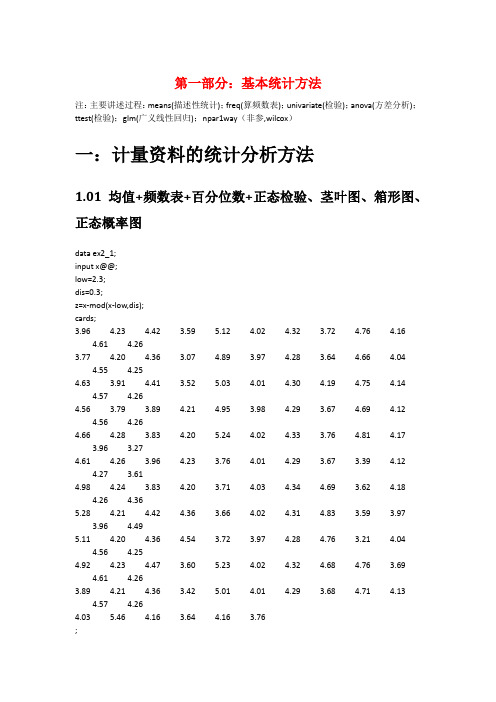
第一部分:基本统计方法注:主要讲述过程:means(描述性统计);freq(算频数表);univariate(检验);anova(方差分析);ttest(检验);glm(广义线性回归);npar1way(非参,wilcox)一:计量资料的统计分析方法1.01均值+频数表+百分位数+正态检验、茎叶图、箱形图、正态概率图data ex2_1;input x@@;low=2.3;dis=0.3;z=x-mod(x-low,dis);cards;3.964.23 4.42 3.595.12 4.02 4.32 3.72 4.76 4.164.61 4.263.774.20 4.36 3.07 4.89 3.97 4.28 3.64 4.66 4.044.55 4.254.63 3.91 4.41 3.525.03 4.01 4.30 4.19 4.75 4.144.57 4.264.56 3.79 3.89 4.21 4.95 3.98 4.29 3.67 4.69 4.124.56 4.264.66 4.28 3.83 4.205.24 4.02 4.33 3.76 4.81 4.173.96 3.274.61 4.26 3.96 4.23 3.76 4.01 4.29 3.67 3.39 4.124.27 3.614.98 4.24 3.83 4.20 3.71 4.03 4.34 4.69 3.62 4.184.26 4.365.28 4.21 4.42 4.36 3.66 4.02 4.31 4.83 3.59 3.973.964.495.11 4.20 4.36 4.54 3.72 3.97 4.28 4.76 3.21 4.044.56 4.254.92 4.23 4.47 3.605.23 4.02 4.32 4.68 4.76 3.694.61 4.263.894.21 4.36 3.425.01 4.01 4.29 3.68 4.71 4.134.57 4.264.035.46 4.16 3.64 4.16 3.76;/*freq语句,算频数表*/proc freq;tables z;run;proc means data=ex2_1n mean std stderr clm;var x;run;data ex2_1;input x f@@;cards;3.07 23.27 33.47 93.67 143.87 224.07 304.27 214.47 154.67 104.87 65.07 45.27 2;run;proc means;freq f;var x;run;/*把freq f改成weight f就是把f当权重或频数来算,f则在0,1之间*//*计算x的95%的置信区间*/proc univariate data=ex2_1;var x;output out=pctpctlpre=ppctlpts=2.5 97.5;run;proc print data=pct;run;/*正态检验、茎叶图、箱形图、正态概率图*/proc univariate data=ex2_1normalplot;var x;run;/*Extreme Observation显示的值是最小的5个极值和最大的5个极值*/1.02几何均值data ex2_5;input x f@@;y=log10(x);cards;10 420 340 1080 10160 11320 15640 141280 2;proc means noprint;/*调用means过程,不显示结果*/var y;freq f;output out=b/*结果输出到数据集b中*/mean=logmean;/*把数据集b中均数的变量名mean改为logmean*/run;data c;/*新建数据集c*/set b;/*调用数据集b*/g=10**logmean;/*计算变量logmean的反对数,该值就是x的几何均数,将该值赋值给变量g*/ proc print data=c;var g;run;/*这个是计算平通平均数的值*/proc means data=ex2_5;var x;freq f;run;1.03已知均值和方差求置信区间-单样本+单样本与总体/*单样本*/data ex3_2;n=10;mean=166.95;std=3.64;t=tinv(0.975,n-1);pts=t*std/sqrt(n);lclm=mean-pts;uclm=mean+pts;proc print;var lclm uclm;run;/*单样本与总体均值*/data ex3_5;n=36;/*样本量*/s_m=130.83;/*样本均值*/std=25.74;/*样本标准差*/p_m=140;/*总体均值*/df=n-1;/*自由度*/t=(s_m-p_m)/(std/sqrt(n));p=(1-probt(abs(t),df))*2;/*根据t值计算p值*/run;proc print;var t p;run;1.06双样本均值相等检验+两组分开+两组一起算+两组样本量不同/*双样本分开算*/data ex3_4;n1=29;n2=32;m1=20.10;m2=16.89;s1=7.02;s2=8.46;ss1=s1**2*(n1-1);ss2=s2**2*(n2-1);sc2=(ss1+ss2)/(n1+n2-2);se=sqrt(sc2*(1/n1+1/n2));t=tinv(0.975,n1+n2-2);lclm=(m1-m2)-t*se;uclm=(m1-m2)+t*se;proc print;var t se lclm uclm;run;/*双样本相减后再算*//*用MEANS作配对资料两个样本均数比较的t检验*/data ex3_6;input x1 x2 @@;d=x1-x2;cards;0.840 0.5800.591 0.5090.674 0.5000.632 0.3160.687 0.3370.978 0.5170.750 0.4540.730 0.5121.200 0.9970.870 0.506;proc means t prt;var d;run;/*用UNIVARIATE过程作配对资料两样本均数比较的t检验*/ proc univariate data=ex3_6;var d;run;/*双样本两组样本量不同*/data ex3_7;input x@@;if _n_<21 then c=1;/*当观测数小于21时,变量c的值为1,表示试验组*/else c=2;/*其余变量c的值为2,表示对照组*/cards;-0.70 -5.60 2.00 2.80 0.70 3.50 4.00 5.80 7.10 -0.502.50 -1.60 1.703.00 0.404.50 4.60 2.50 6.00 -1.403.70 6.50 5.00 5.20 0.80 0.20 0.60 3.40 6.60 -1.106.00 3.80 2.00 1.60 2.00 2.20 1.20 3.10 1.70 -2.00;proc ttest;/*调用ttest过程*/var x;/*定义分析变量为x*/class c;/*定义分组变量为c*/run;1.08-1.13anova方差分析过程+一维分组+二维分组+三维分组/*只有一组分组因素*/data ex4_2;input x c @@;cards;3.53 1 2.42 2 2.86 3 0.89 44.59 1 3.36 2 2.28 3 1.06 44.34 1 4.32 2 2.39 3 1.08 42.66 1 2.34 2 2.28 3 1.27 43.59 1 2.68 2 2.48 3 1.63 43.13 1 2.95 2 2.28 3 1.89 43.30 1 2.36 2 3.48 3 1.31 44.04 1 2.56 2 2.42 3 2.51 43.53 1 2.52 2 2.41 3 1.88 43.56 1 2.27 2 2.66 3 1.41 43.85 1 2.98 2 3.29 3 3.19 44.07 1 3.72 2 2.70 3 1.92 41.37 12.65 2 2.66 3 0.94 43.93 1 2.22 2 3.68 3 2.11 42.33 1 2.90 2 2.65 3 2.81 42.98 1 1.98 2 2.66 3 1.98 44.00 1 2.63 2 2.32 3 1.74 43.55 1 2.86 2 2.61 3 2.16 42.64 1 2.93 23.64 3 3.37 42.56 1 2.17 2 2.58 3 2.97 43.50 1 2.72 2 3.65 3 1.69 43.25 1 1.56 2 3.21 3 1.19 42.96 13.11 2 2.23 3 2.17 44.30 1 1.81 2 2.32 3 2.28 43.52 1 1.77 2 2.68 3 1.72 43.93 1 2.80 2 3.04 3 2.47 44.19 1 3.57 2 2.81 3 1.02 42.96 1 2.97 23.02 3 2.52 44.16 1 4.02 2 1.97 3 2.10 42.59 1 2.31 2 1.68 33.71 4;proc anova;/*调用anova过程*/class c;/*定义分组变量为c*/model x=c;/*定义模型,分析g对x的影响*/means c/dunnett;/*用LSD法对多组均数过行两两比较*/means c/hovtest;/*作方差齐性检验,默认levene法,p值大于0.05,则认为是g组方差相等*/run;quit;/*有两组分组因素*/data ex4_4;input x a b@@;cards;0.82 1 10.65 2 10.51 3 10.73 1 20.54 2 20.23 3 20.43 1 30.34 2 30.28 3 30.41 1 40.21 2 40.31 3 40.68 1 50.43 2 50.24 3 5;proc anova;class a b;/*定义分组变量a和b*/model x=a b;/*定义模型,分析a和b对x影响*/means a/snk;/*用SNK法对变量a的多组均数进行两两比较*/run;quit;1.15嵌套设计资料的方差分析glm过程一级因素+二组因素(glm过程要先class再model)/*嵌套设计资料的方差分析*/data ex11_6;input x a b @@;cards;82 1 184 1 191 1 288 1 285 1 383 1 365 2 461 2 462 2 559 2 556 2 660 2 671 3 767 3 775 3 878 3 885 3 989 3 9;proc glm;/*调用glm过程*/class a b;/*定义分组变量为a和b*/model x=a a(b);/*定义模型,以a为一组因素,b为二级因素*/run;quit;1.17重复测量资料的方差分析data ex12_2;input t1 t2 g@@;/*确定变量名称,t1和t2分别为两个时间点的分析变量,g为处理因素变量,b为区组变量*/cards;130 114 1124 110 1136 126 1128 116 1122 102 1118 100 1116 98 1138 122 1126 108 1124 106 1118 124 2132 122 2134 132 2114 96 2118 124 2128 118 2118 116 2132 122 2120 124 2134 128 2;proc glm;/*调用glm过程*/class g;/*定义分组变量g*/model t1 t2=g;/*定义模型,分析g对变量t1和t2的影响*/repeated time 2/*命名重复因子为time,有2个水平*/contrast(1)/*表示以第一时间点为对照点*//summary;/*考察不同时间点与对照时间点比较的结果*/run;quit;data ex12_3;input t0-t4 g@@;cards;120 108 112 120 117 1118 109 115 126 123 1119 112 119 124 118 1121 112 119 126 120 1127 121 127 133 126 1121 120 118 131 137 2122 121 119 129 133 2128 129 126 135 142 2117 115 111 123 131 2118 114 116 123 133 2131 119 118 135 129 3129 128 121 148 132 3123 123 120 143 136 3123 121 116 145 126 3125 124 118 142 130 3;proc glm;class g;model t0-t4=g;repeated time 5/*命名重复因子为time,有2个水平*/contrast(1);run;quit;二:计数资料的统计分析方法2.1四格表资料的卡方检验data ex7_1;input r c f@@;/*确定变量名称,r为行变量,c为列变量,f为频数变量*/ cards;1 1 991 2 52 1 752 2 21;proc freq;/*调用freq过程*/weight f;/*定义f为频数变量*/tables r*c/*作r*c的列联表*//chisq/*对列联表作卡方检验*/expected;/*输出每个格的理论频数*/run;2.5阳性事件发生的概率(二项分布)data ex6_1;do x=6 to 8;/*建立循环,变量x从6到8*/p1=probbnml(0.7,10,x);/*计算二项分布随机变量不大于x的概率*/p2=probbnml(0.7,10,x-1);/*计算二项分布随机变量不大于x-1的概率*/p=p1-p2;*/计算出现x的概率*/output;/*结果输出*/end;proc print;var x p;run;2.6正态分布法计算总体率的可信区间data ex6_3;n=100;x=55;p=x/n;sp=sqrt(p*(1-p)/n);u=probit(0.975);usp=u*sp;lclm=p-usp;uclm=p+usp;proc print;var n p sp lclm uclm;run;2.7样本率与总体率的比较(直接法——单侧检验)data ex6_4;d=probbnml(0.55,10,8);p=1-d;proc print;var p;run;2.8样本率与总体率的比较(直接法——双侧检验)data ex6_5;p01=probbnml(0.6,10,9);p02=probbnml(0.6,10,8);p0=p01-p02;/*计算出现9的概率*/do i=0to10;/*建立循环,变量i从0到10*/p11=probbnml(0.6,10,i);p12=probbnml(0.6,10,i-1);p1=p11-p12;/*计算出现i的概率*/if i=0then p1=p11; /*定义出现0的概率*/if p1<=p0 then output; /*如果出现i的概率小于出现9的概率,则保留在数据集中*/ end;proc means sum;var p1;run;2.9两个样本率比较的z检验data ex6_7;n1=120;n2=110;x1=36;x2=22;p1=x1/n1;p2=x2/n2;pc=(x1+x2)/(n1+n2);/*计算合并发生率*/sp=sqrt(pc*(1-pc)*(1/n1+1/n2));/*计算两个率相差的标准误差*/u=(p1-p2)/sp;/*计算u值*/p=(1-probnorm(abs(u)))*2;/*计算p值*/format u p 5.4;/*输出格式为小数点后保留4位*/proc print;var pc sp u p;run;2.10.Poisson分布的样本均数与总体均数比较(直接法)data ex6_12;n=120;/*确定样本例数*/pai=0.008; /*确定总体率*/lam=n*pai; /*计算总体均数lamda*/x=4; /*确定实际发生数*/p=1-poisson(lam,x-1);/*计算实际发生数所对应的概率*/proc print;var lam p;run;2.11 Poisson分布的样本均数与总体均数比较(正态近似法)data ex6_12;n=25000;/*样本量*/x=123; /*样本均数*/pi=0.003; /*确定总体率*/lam=n*pi; /*计算总体均数*/u=(x-lam)/sqrt(lam*(1-pi)); /*计算u值*/p=1-probnorm(abs(u)); /*计算u值所对应的p值*/proc print;var lam u p;run;2.14负二项分布的参数估计data ex6_16;input x f@@;cards;0 301 142 83 44 25 06 2;proc univariate;var x;freq f;output out=mv2var=v;run;data k;set mv2;k=mu**2/(v-mu);proc print;var mu k;run;三、非参数统计方法3.2单个样本中位数和总体中位数比较data ex8_2;input x1@@;median=45.30;/*假设中位数为45.30*/d=x1-median; /*计算x1和假设中位数的差值*/cards;44.21 45.30 46.39 49.47 51.05 53.1653.26 54.37 57.16 67.37 71.05 87.37;proc univariate; /*调用univariate过程度*/var d;run;proc means median; /*调用means过程计算x1实际的中位数*/var x1;run;3.3两个独立样本比较的Wilcoxon秩和检验(R对应函数wilcox.test())data ex8_3;input x c @@;/*确定变量名称,x、c分别为分析变量和分组变量(类别多于两类一样的写法)*/2.78 13.23 14.20 14.87 15.12 16.21 17.18 18.05 18.56 19.60 13.23 23.50 24.04 24.15 24.28 24.34 24.47 24.64 24.75 24.82 24.95 25.10 2;proc npar1way wilcoxon;/*调用npar1way过程,进行wilcoxon分析*/var x;/*定义分析变量为x*/class c;/*定义分组变量为c*/run;3.4等级资料的两样本比较data ex8_4;input c g f@@;/*确定变量名称,f为频数,c为分类,g为要分析的变量(分类多种类似)*/ cards;1 1 11 2 81 3 161 4 101 5 42 1 22 2 232 3 112 5 0;proc npar1way wilcoxon;/*调用npar1way过程,进行wilcoxon分析*/freq f;/*确定频数变量为f*/var g;/*定义分析变量g*/class c;/*定义分组变量c*/run;第二部分:多元统计分析方法注:主要讲述过程:reg(回归),corr(相关分析),nlin(对数曲线回归),logistic(逻辑回归),phreg(条件logistic回归分析+cox回归),life test(生存分析),discrim(判别分析),stepdisc(逐步回归),cluster(聚类),varclus(指标聚类),princomp(主成分分析),factor(因子分析),cancorr(典型相关分析)一:回归和相关分析1.1两个变量的直线回归分析data ex9_1;input x y;/*确定变量名称*/cards;13 3.5411 3.019 3.096 2.488 2.5610 3.3612 3.187 2.65;proc reg;/*调用reg过程*/model y=x;/*定义模型,以y为应变量,以x为自变量*//*在model语句后面加上选项,得到一些有用的统计量,常用的有:stb(输出标准化偏回归系数)、p(输出每个观测的实际值、预测值和残差)、cli(输出每个观测预测值均数的双侧95%置信区间)、clm(输出每个观测预测值的双侧95%置信范围)*//*例如:model y=x /stb p cli */plot y*x;/*画出散点图*/run;1.2两个变量的直线相关分析data ex9_5;input x y;cards;43 217.2274 316.1851 231.1158 220.9650 254.7065 293.8454 263.2857 271.7367 263.4669 276.5380 341.1548 261.0038 213.2085 315.1254 252.08;proc corr;/*若要求作spearman相关分析,则可以写成proc corr spearman */ var x y;run;/*得到一个相关系数矩阵*/1.4加权直线加回data ex9_9;input x y;w=1/(x*x); /*设置权重变量w*/cards;0.11 4.000.12 5.100.21 9.500.30 9.000.34 17.200.44 14.000.56 18.900.60 29.400.69 22.100.80 41.50;proc reg;weight w;/*定义权重变量w*/model y=x;/*定义模型,以y为因变量,以x为自变量*/run;1.5两个直线回归系数的比较data ex9_12;input x y c@@;cards;13 3.54 111 3.01 19 3.09 16 2.48 18 2.56 110 3.36 112 3.18 17 2.65 110 3.01 29 2.83 211 2.92 212 3.09 215 3.98 216 3.89 28 2.21 27 2.39 210 2.74 215 3.36 2;proc glm;class c;model y=x c x*c;/*定义模型,分析x、c以及x和c的交互作用对y的影响,即判断两总体直线回归系数是否相同*/run;proc glm;class c;model y=x c;/*上一步已排除协变量的影响,然后再分析两分析变量是否来自同一总体*/run;1.6两个变量的对数曲线回归data ex9_13;input x y;cards;0.005 34.110.050 57.990.500 94.495.000 128.5025.000 169.98;proc nlin;/*调用nlin过程*/parms a=0 b=0; /*定义初始值*/model y=a+b*log10(x); /*定义对数模型,以y为因变以量,x为自变量*/ run;1.7两个变量的指数曲线回归分析data ex9_14;input x y;cards;2 545 507 4510 3714 3519 2526 2031 1634 1838 1345 852 1153 860 465 6;proc nlin;parms a=4 b=0.03;/*定义初始值*/model y=exp(a+b*x);/*定义指数模型,以y为因变量,x为自变量*/run;1.8多元回归data ex15_1;input x1-x4 y@@;/*确定变量名称,x1,x2,x3,x4分别为自变量,y为应变量*/ cards;5.68 1.90 4.53 8.20 11.203.79 1.64 7.32 6.90 8.806.02 3.56 6.95 10.80 12.304.85 1.075.88 8.30 11.604.60 2.32 4.05 7.50 13.406.05 0.64 1.42 13.60 18.304.90 8.50 12.60 8.50 11.107.08 3.00 6.75 11.50 12.103.85 2.11 16.28 7.90 9.604.65 0.63 6.59 7.10 8.404.59 1.97 3.61 8.70 9.304.29 1.97 6.61 7.80 10.607.97 1.93 7.57 9.90 8.406.19 1.18 1.42 6.90 9.606.13 2.06 10.35 10.50 10.905.71 1.78 8.53 8.00 10.106.40 2.40 4.53 10.30 14.806.06 3.67 12.797.10 9.105.09 1.03 2.53 8.90 10.806.13 1.71 5.28 9.90 10.205.78 3.36 2.96 8.00 13.605.43 1.13 4.31 11.30 14.906.50 6.21 3.47 12.30 16.007.98 7.92 3.37 9.80 13.2011.54 10.89 1.20 10.50 20.005.84 0.92 8.616.40 13.303.84 1.20 6.45 9.60 10.40;proc reg;model y=x1-x4;/*也可以写成model y=x1 x2 x3 x4;*/run;1.9逐步回归data ex12_2;input x1-x4 y@@;cards;5.68 1.90 4.53 8.20 11.203.79 1.64 7.32 6.90 8.806.02 3.56 6.95 10.80 12.304.85 1.075.88 8.30 11.604.60 2.32 4.05 7.50 13.406.05 0.64 1.42 13.60 18.304.90 8.50 12.60 8.50 11.107.08 3.00 6.75 11.50 12.103.85 2.11 16.28 7.90 9.604.65 0.63 6.59 7.10 8.404.59 1.97 3.61 8.70 9.304.29 1.97 6.61 7.80 10.607.97 1.93 7.57 9.90 8.406.19 1.18 1.42 6.90 9.606.13 2.06 10.35 10.50 10.905.71 1.78 8.53 8.00 10.106.40 2.40 4.53 10.30 14.806.06 3.67 12.797.10 9.105.09 1.03 2.53 8.90 10.806.13 1.71 5.28 9.90 10.205.78 3.36 2.96 8.00 13.605.43 1.13 4.31 11.30 14.906.50 6.21 3.47 12.30 16.007.98 7.92 3.37 9.80 13.2011.54 10.89 1.20 10.50 20.005.84 0.92 8.616.40 13.303.84 1.20 6.45 9.60 10.40;proc reg;model y=x1-x4/selection=stepwise/*定义模型,以y因变量,x1-x4为变量进行多元回归分析*/ sle=0.10/*定义入先变量的界值*/sls=0.10;/*定义剔除变量的界值*/run;三:logistic回归3.1 两个变量logistic回归分析data ex16_1;input y x1 x2 f@@;/*确定变量名称,y为发病情况,x1为吸烟情况,x2为饮酒情况,f为发生频数*/cards;1 0 0 631 0 1 631 1 0 441 1 1 2650 0 0 1360 0 1 1070 1 0 570 1 1 151;proc logistic;/*调用logistic过程*/freq f;/*定义频数变量f*/model y=x1 x2;/*定义模型,以y为因变量,x1和x2为自变量*/run;3.2 1:M配对资料的条件logistic回归分析data ex16_3;input i y x1-x6 @@;/*确定变量名称,i为区组变量,y为病人情况,1为病例,0为对照,x1-x6为危险因素*/t=2-y;/*定义时间变量*/cards;1 1 3 5 1 1 1 01 0 1 1 1 3 3 01 0 1 1 1 3 3 02 1 13 1 1 3 02 0 1 1 13 2 02 0 1 2 13 2 03 1 14 1 3 2 03 0 1 5 1 3 2 03 0 14 1 3 2 04 1 1 4 1 2 1 14 0 2 1 1 3 2 05 1 2 4 2 3 2 0 5 0 1 2 1 3 3 05 0 2 3 1 3 2 06 1 1 3 1 3 2 1 6 0 1 2 1 3 2 06 0 1 3 2 3 3 07 1 2 1 1 3 2 1 7 0 1 1 1 3 3 07 0 1 1 1 3 3 08 1 1 2 3 2 2 0 8 0 1 5 1 3 2 08 0 1 2 1 3 1 09 1 3 4 3 3 2 0 9 0 1 1 1 3 3 09 0 1 4 1 3 1 010 1 1 4 1 3 3 1 10 0 1 4 1 3 3 010 0 1 2 1 3 1 011 1 3 4 1 3 2 0 11 0 3 4 1 3 1 011 0 1 5 1 3 1 012 1 1 4 3 3 3 0 12 0 1 5 1 3 2 012 0 1 5 1 3 3 013 1 1 4 1 3 2 0 13 0 1 1 1 3 1 013 0 1 1 1 3 2 014 1 1 3 1 3 2 1 14 0 1 1 1 3 1 014 0 1 2 1 3 3 015 1 1 4 1 3 2 0 15 0 1 5 1 3 3 015 0 1 5 1 3 3 016 1 1 4 2 3 1 0 16 0 2 1 1 3 3 016 0 1 1 3 3 2 017 1 2 3 1 3 2 0 17 0 1 1 2 3 2 017 0 1 2 1 3 2 018 1 1 4 1 3 2 0 18 0 1 1 1 2 1 0 18 0 1 2 1 3 2 019 0 1 1 1 2 1 019 0 2 2 2 3 1 020 1 1 4 2 3 2 120 0 1 5 1 3 3 020 0 1 4 1 3 2 021 1 1 5 1 2 1 021 0 1 4 1 3 2 021 0 1 2 1 3 2 122 1 1 2 2 3 1 022 0 1 2 1 3 2 022 0 1 1 1 3 3 023 1 1 3 1 2 2 023 0 1 1 1 3 1 123 0 1 1 2 3 2 124 1 1 2 2 3 2 124 0 1 1 1 3 2 024 0 1 1 2 3 2 025 1 1 4 1 1 1 125 0 1 1 1 3 2 025 0 1 1 1 3 3 0;proc phreg;/*调用phreg过程*/model t*y(0)=x1-x6/*定义模型,以t为时间变量,y为截尾变量,x1-x6为自变量*//selection=stepwise/*选择逐步回归方法筛选变量*/sle=0.1sls=0.1/*入选和剔除的界值均为0.1*/ties=discrete;/*用离散logistic模型替代比例危险模型*/strata i;/*定义区组变量*/run;2.3 应变量为多分类资料的logistic回归data ex16_5;input x1 x2 y f;/*x1是两个社区,x2是性别,Y是获取健康知识途径(传统大众媒介=1,网络=2,社区宣传=3,f为频数)*/cards;0 0 1 200 0 2 350 0 3 260 1 1 100 1 2 270 1 3 571 0 1 421 02 171 1 1 161 12 121 1 3 26;proc logistic;freq f;/*定义频数变量为f*/model y(ref='3')/*定义模型,以y为因变量,ref语句指时参照的类别为“社区宣传”,最后得到结果均为与“社区宣传”相对应*/=x1 x2/*定义x1和x2为自变量*//link=glogit;/*指定多分类应变量回归模型*/run;四:生存分析4.1乘积极限法估计生存率,例17-2甲、乙两种手术方法的生存率估计data ex17_2;input t d@@;/*确定变量名称,t为时间变量,d为截尾变量*/cards;1 13 15 15 15 16 16 16 17 18 110 110 114 017 119 020 022 026 034 134 044 159 1;proc lifetest;/*调用lifetest过程*/time t*d(0);/*定义模型,以t为时间变量,d为截尾变量,变量值为0表示截尾数据*/ run;4.2寿命表法估计生存率data ex17_3;input t d f@@;cards;0 0 00 1 4561 0 391 1 2262 0 222 1 1523 0 233 1 1714 0 244 1 1355 0 1075 1 1256 0 1336 1 837 0 1027 1 748 0 688 1 519 0 649 1 4210 0 4510 1 4311 0 5311 1 3412 0 3312 1 1813 0 2714 0 3314 1 615 0 2015 1 0;proc lifetest method=life/*调用lifetest过程,指定用寿命表法估计生存率*/ width=1;/*表示每间隔1估计生存率*/freq f;/*表示以f为频数变量*/time t*d(0);/*定义模型,以t为时间变量,d为截尾变量,变量值为0表示截尾数据*/ run;4.3生存曲线比较的log-rank检验及制作生存曲线data ex17_4;input t d g @@;cards;1 1 13 1 15 1 15 1 15 1 16 1 16 1 16 1 17 1 18 1 110 1 110 1 114 0 117 1 119 0 120 0 122 0 126 0 131 0 134 1 134 0 144 1 159 1 11 1 21 1 22 1 23 1 23 1 24 1 24 1 24 1 26 1 26 1 28 1 29 1 29 1 210 1 211 1 212 1 213 1 215 1 217 1 218 1 2;proc lifetest plot=(s);/*调用lifetest过程并做生存曲线图*/ time t*d(0);strata g;/*定义变量g为分组变量*/run;4.4.cox回归分析data ex17_5;input x1-x6 t y @@;cards;54 0 0 1 1 0 52 057 0 1 0 0 0 51 058 0 0 0 1 1 35 143 1 1 1 1 0 103 048 0 1 0 0 0 7 140 0 1 0 0 0 60 044 0 1 0 0 0 58 036 0 0 0 1 1 29 139 1 1 1 0 1 70 042 0 1 0 0 1 67 042 0 1 0 0 0 66 042 1 0 1 1 0 87 051 1 1 1 0 0 85 055 0 1 0 0 1 82 052 1 1 1 0 1 74 0 48 1 1 1 0 0 63 0 54 1 0 1 1 1 101 0 38 0 1 0 0 0 100 0 40 1 1 1 0 1 66 1 38 0 0 0 1 0 93 0 19 0 0 0 1 0 24 1 67 1 0 1 1 0 93 0 37 0 0 1 1 0 90 0 43 1 0 0 1 0 15 149 0 0 0 1 0 3 150 1 1 1 1 1 87 0 53 1 1 1 0 0 120 0 32 1 1 1 0 0 120 0 46 0 1 0 0 1 120 043 1 0 1 1 0 120 044 1 0 1 1 0 120 0 62 0 0 0 1 0 120 0 40 1 1 1 0 1 40 1 50 1 0 0 1 0 26 1 33 1 1 0 0 0 120 0 57 1 1 1 0 0 120 0 48 1 0 0 1 0 120 0 28 0 0 0 1 0 3 1 54 1 0 1 1 0 120 1 35 0 1 0 1 1 7 1 47 0 0 0 1 0 18 1 49 1 0 1 1 0 120 0 43 0 1 0 0 0 120 0 48 1 1 0 0 0 15 1 44 0 0 0 1 0 4 1 60 1 1 1 0 0 120 0 40 0 0 0 1 0 16 1 32 0 1 0 0 1 24 1 44 0 0 0 1 1 19 1 48 1 0 0 1 0 120 0 72 0 1 0 1 0 24 1 42 0 0 0 1 0 2 1 63 1 0 1 1 0 120 0 55 0 1 1 0 0 12 1 39 0 0 0 1 0 5 1 44 0 0 0 1 0 120 0 42 1 1 1 0 0 120 061 0 1 0 1 0 40 145 1 0 1 1 0 108 038 0 1 0 0 0 24 162 0 0 0 1 0 16 1;proc phreg;model t*y(1)=x1-x6/*定义模型,以t为时间变量,y为截尾变量,变量值1表示截尾数据,x1-x6为危险因素*//selection=stepwisesle=0.05sls=0.05;run;五:判别和聚类分析5.1判别分析data ex18_4;input x1-x4 g; /*确定变量名称,x1-x4为用于进行判别分析的指标,g为分组变量*/ cards;6.0 -11.5 19 90 1-11.0 -18.5 25 -36 390.2 -17.0 17 3 2-4.0 -15.0 13 54 10.0 -14.0 20 35 20.5 -11.5 19 37 3-10.0 -19.0 21 -42 30.0 -23.0 5 -35 120.0 -22.0 8 -20 3-100.0 -21.4 7 -15 1-100.0 -21.5 15 -40 213.0 -17.2 18 2 2-5.0 -18.5 15 18 110.0 -18.0 14 50 1-8.0 -14.0 16 56 10.6 -13.0 26 21 3-40.0 -20.0 22 -50 3;proc discrim;class g;/*定义分组变量为g*/var x1-x4;/*定义用于分析的指标变量为x1-x4*/run;(结果横向是真实值,竖向的预测值)5.2逐步判别分析data ex18_5;input x1-x4 g;cards;6.0 -11.5 19 90 1-11.0 -18.5 25 -36 390.2 -17.0 17 3 2-4.0 -15.0 13 54 10.0 -14.0 20 35 20.5 -11.5 19 37 3-10.0 -19.0 21 -42 30.0 -23.0 5 -35 120.0 -22.0 8 -20 3-100.0 -21.4 7 -15 1-100.0 -21.5 15 -40 213.0 -17.2 18 2 2-5.0 -18.5 15 18 110.0 -18.0 14 50 1-8.0 -14.0 16 56 10.6 -13.0 26 21 3-40.0 -20.0 22 -50 3;proc stepdisc /*调用stepdisc过程*/slentry=0.2/*确定入选标准为0.2*/slstay=0.3;/*确定剔除标准为0.3*/class g;/*定义分组变量为g*/var x1-x4;/*定义用于分析的指标变量为x1-x4*/run;(筛选出变量后,调用discrim过程对筛选出的变量作判别分析,即先做5.2再做5.1)5.3作样品聚类和指标聚类data ex19_3;input x1-x9;cards;46 25 5 2138 1.68 0.35 8.11 4 4 35 12 20 3510 2.76 1.43 6.84 3 3 52 25 20 2784 2.19 0.54 4.11 3 3 32 7 20 2451 1.93 0.47 11.45 9 6 38 22 0 3247 2.56 0.80 11.68 5 5 51 31 30 3710 2.92 0.37 11.60 2 2 40 9 10 3194 2.51 0.40 11.40 5 5 34 17 20 4658 3.67 0.46 11.35 3 3 50 29 0 5019 3.95 0.47 13.45 10 8 42 20 20 7482 5.89 0.12 13.11 0 0 57 30 15 3800 2.99 0.19 10.76 2 236 15 20 2478 1.95 0.25 10.00 0 037 12 0 3827 3.01 0.82 10.50 4 4 52 32 0 2984 2.35 0.16 11.15 3 3 52 32 10 3749 2.95 0.72 11.45 11 10 42 27 30 4941 3.89 0.73 13.80 7 6 44 27 20 3948 3.11 0.33 13.65 16 14 40 21 5 3360 2.64 0.37 11.40 0 0 38 21 5 2936 2.31 0.69 11.40 1 1 44 27 20 6851 5.39 0.99 12.28 7 6 43 27 0 3926 3.09 0.47 11.95 0 0 26 10 3 4381 3.45 0.52 11.80 7 5 37 18 20 7142 5.62 0.85 11.81 5 5 28 9 20 2612 2.06 0.37 11.65 1 1 25 9 30 2638 2.08 0.78 12.25 1 1 34 14 20 4322 3.40 0.41 15.00 5 5 50 32 20 2862 2.25 0.69 8.80 2 2;proc cluster/*调用cluster过程*/method=average;/*采用类平均法进行聚类*/var x1-x9;/*定义用于分析的指标变量x1-x9*/run;proc treegraphics haxis=axis1 horizontal;/*调用tree过程输出聚类图,并将图横向输出*/ run;/*对各个指标聚类,即对9个变量聚类*/proc varclus;/*调用varclus过程*/var x1-x9;/*定义用于分析的指标变量x1-x9*/run;六、主成分分析和因子分析6.1主成分分析data ex20_1;input x1-x6;cards;92 77 80 95 99 12697 75 77 80 95 12595 80 70 78 89 12075 75 73 88 98 11092 68 72 79 88 11390 85 80 70 78 10372 93 75 77 80 10088 70 76 72 81 10264 70 69 85 93 10570 73 70 87 84 10078 69 75 73 89 9778 72 71 68 75 9675 64 63 76 73 9284 66 77 55 65 7670 64 51 60 67 8858 72 75 62 52 7582 73 40 50 48 6145 65 42 47 43 60;proc princomp;/*调用princomp过程,对6个变量做主成分分析,结果包括主成分累积贡献率,特征向量矩阵*/run;6.2因子分析data ex20_2;input x1-x9;cards;4.34 389 99.06 1.23 25.46 93.15 3.56 97.51 61.663.45 271 88.28 0.85 23.55 94.31 2.44 97.94 73.334.38 385 103.97 1.21 26.54 92.53 4.02 98.484.18 377 99.48 1.19 26.89 93.86 2.92 99.41 63.164.32 378 102.01 1.19 27.63 93.18 1.99 99.71 80.004.13 349 97.55 1.10 27.34 90.63 4.38 99.03 63.164.57 361 91.66 1.14 24.89 90.60 2.73 99.69 73.534.31 209 62.18 0.52 31.74 91.67 3.65 99.48 61.114.06 425 83.27 0.93 26.56 93.81 3.09 99.48 70.734.43 458 92.39 0.95 24.26 91.12 4.21 99.76 79.074.13 496 95.43 1.03 28.75 93.43 3.50 99.10 80.494.10 514 92.99 1.07 26.31 93.24 4.22 100.00 78.954.11 490 80.90 0.97 26.90 93.68 4.97 99.77 80.533.53 344 79.66 0.68 31.87 94.77 3.59 100.00 81.974.16 508 90.98 1.01 29.43 95.75 2.77 98.72 62.864.17 545 92.98 1.08 26.92 94.89 3.14 99.41 82.354.16 507 95.10 1.01 25.82 94.41 2.80 99.35 60.614.86 540 93.17 1.07 27.59 93.47 2.77 99.80 70.215.06 552 84.38 1.10 27.56 95.15 3.10 98.63 69.234.03 453 72.69 0.90 26.03 91.94 4.50 99.05 60.424.15 529 86.53 1.05 22.40 91.52 3.84 98.58 68.423.94 515 91.01 1.02 25.44 94.88 2.56 99.36 73.914.12 552 89.14 1.10 25.70 92.65 3.87 95.52 66.674.42 597 90.18 1.18 26.94 93.03 3.76 99.28 73.813.05 437 78.81 0.87 23.05 94.46 4.03 96.223.94 477 87.34 0.95 26.78 91.784.57 94.28 87.344.14 638 88.57 1.27 26.53 95.16 1.67 94.50 91.673.87 583 89.82 1.16 22.66 93.43 3.55 94.49 89.074.08 552 90.19 1.10 22.53 90.36 3.47 97.88 87.144.14 551 90.81 1.09 23.06 91.65 2.47 97.72 87.134.04 574 81.36 1.14 26.65 93.74 1.61 98.20 93.023.93 515 76.87 1.02 23.88 93.82 3.09 95.46 88.373.90 555 80.58 1.10 23.08 94.38 2.06 96.82 91.793.62 554 87.21 1.10 22.50 92.43 3.22 97.16 87.773.75 586 90.31 1.12 23.73 92.47 2.07 97.74 93.893.77 627 86.47 1.24 23.22 91.17 3.40 98.98 89.80;proc factor/*调用factor过程*/n=4;/*确定因子数为4,如果不写就默认为3*/run;proc factorn=4rotate=quartimax;/*因子旋转的方法为四次方最大正交旋转*/run;七、典型相关分析(具体解释看ppt“SAS-典型相关分析(可以先上本章_再上对应分析)”)data ex21_1;input x1-x4 y1-y4;cards;1210 120.7 23.4 59.8 11.3 67.6 1.92 2.71 1040 121.2 22.9 59.0 10.1 66.5 1.92 2.60 1620 121.5 24.6 59.5 9.5 67.8 1.95 2.64 1690 122.5 24.4 60.7 11.0 69.2 2.08 2.64 1150 122.7 27.2 64.5 10.5 69.1 2.19 2.84 1150 123.2 20.0 56.1 10.4 59.3 1.83 2.61 1460 123.3 24.9 58.4 10.5 69.0 2.01 2.72 1190 123.4 21.8 59.0 10.6 67.4 1.90 2.71 1840 123.9 23.5 60.2 9.6 67.1 2.00 2.84 1250 124.5 25.2 63.0 11.2 67.8 2.05 2.78 1480 124.8 22.3 58.1 10.7 67.9 2.05 2.73 1310 124.9 22.0 58.0 10.5 67.8 1.98 2.68 1660 125.3 24.7 60.0 10.8 69.3 1.95 2.80 1580 125.6 22.8 59.0 9.4 69.1 2.00 2.65 1460 125.8 25.7 61.0 10.2 69.6 1.95 2.70 1240 126.0 30.2 68.0 9.2 67.1 2.14 2.88 1100 126.2 25.2 60.5 9.8 68.4 1.98 2.72 1250 126.8 23.6 58.5 10.2 67.5 1.94 2.74 1270 127.1 23.0 57.7 10.8 69.8 1.90 2.78 1300 127.6 24.3 59.0 10.3 67.9 1.93 2.84 1350 127.7 24.1 60.0 11.0 69.7 2.03 2.77 1250 128.3 21.6 55.5 10.4 68.5 1.83 2.70 1720 128.5 27.1 62.0 11.4 71.2 2.03 2.75 1480 128.5 22.6 57.4 10.0 67.3 2.04 2.83 1380 129.4 24.9 60.5 11.5 69.8 2.04 2.76 1170 129.0 26.7 63.7 9.6 67.4 2.13 2.98 1640 129.8 26.1 62.0 9.8 71.0 2.00 2.84 1640 131.6 28.7 62.8 9.7 70.7 1.89 2.89 1150 130.2 25.0 58.6 10.5 71.8 1.96 2.78 1430 130.5 26.1 60.7 10.8 68.6 2.05 2.77 1150 130.6 23.4 54.4 11.8 69.2 1.96 2.78 1150 131.4 25.5 63.2 10.2 70.4 2.05 2.84 1320 131.6 25.6 58.9 10.9 70.2 2.06 2.86 1360 131.7 27.4 62.0 10.9 73.5 1.99 2.70 1460 132.0 26.3 61.5 11.1 71.2 2.17 2.13 1380 132.2 25.7 61.4 10.1 70.1 1.96 2.83 1300 132.5 24.5 57.0 10.8 71.8 2.02 2.84 1220 132.7 27.0 61.3 10.1 72.2 2.08 2.80 1320 132.9 25.2 60.5 11.2 73.1 2.01 2.73 1910 133.1 30.1 67.0 9.0 87.1 2.15 2.97 1800 133.5 26.5 62.5 9.8 71.7 2.07 2.82 1560 133.6 24.8 58.5 10.3 72.2 1.93 2.79 1840 134.0 26.0 60.5 10.4 73.0 1.98 2.741590 134.4 25.5 60.7 9.6 69.9 1.99 2.81 1430 134.1 26.6 63.0 11.2 72.2 2.06 2.90 1760 134.6 32.5 66.0 9.9 87.4 2.61 2.98 1470 135.3 27.9 61.8 10.1 73.3 2.20 2.78 1580 135.6 28.1 65.8 9.8 73.1 2.05 2.89 1580 136.5 28.2 62.0 11.8 72.9 2.17 2.92 1840 137.1 27.6 62.8 9.5 72.4 2.11 2.91 1810 137.4 28.3 62.5 9.4 74.2 2.06 3.00 1850 138.1 29.5 62.4 9.7 72.3 2.12 4.02 2120 140.0 34.9 68.8 9.5 87.9 2.74 4.15 1760 140.7 32.0 64.4 10.2 74.0 2.17 4.05 1800 141.0 32.5 63.8 9.5 88.2 2.65 4.08 1260 141.7 29.1 65.0 9.7 88.2 2.68 2.90 1860 142.4 19.3 70.0 10.1 89.6 2.71 4.06 1800 144.7 27.0 58.3 10.8 74.8 2.10 2.82 1470 136.8 26.3 61.4 10.0 72.2 2.07 2.93 1260 121.1 22.9 59.0 10.6 66.3 2.05 2.76 1570 132.7 25.3 58.6 11.5 73.6 2.16 2.78 1290 125.0 25.7 60.5 10.1 68.8 2.00 2.69 1580 133.2 27.3 60.7 9.6 71.7 2.11 2.85 1690 132.8 28.6 64.7 9.6 72.9 2.19 4.08 1670 131.6 25.4 59.7 10.6 69.8 2.14 2.76 1300 133.1 25.9 58.0 10.1 69.7 2.12 2.83 1610 134.0 25.8 59.6 9.4 70.8 2.10 2.88 1580 134.3 26.3 61.2 10.2 72.2 2.14 2.84 1570 129.1 27.7 62.2 11.1 72.9 2.09 2.93 1660 140.1 32.1 67.0 9.3 87.1 2.15 4.03 1040 132.6 27.9 62.0 10.3 72.5 2.08 2.81 1290 128.3 23.6 58.5 9.3 69.0 1.97 2.76 1980 145.8 34.5 68.0 9.8 89.7 2.68 4.25 1210 133.3 25.6 61.5 9.9 71.0 2.11 2.82 1300 134.3 25.6 61.0 10.5 73.2 2.02 2.83 1310 138.1 27.8 61.2 9.9 73.5 2.09 2.78 1590 135.6 25.9 59.6 9.6 72.8 2.10 2.91 1270 128.3 24.1 58.5 10.3 69.2 1.92 2.77 1310 129.7 24.7 61.7 10.1 69.4 2.03 2.80 2280 143.6 37.6 70.0 9.7 88.8 2.17 4.18 1580 136.6 32.3 67.2 10.3 87.1 2.66 4.04 2370 147.4 38.8 73.0 10.8 90.7 2.82 4.38 ;proc cancorr;/*调用cancorr过程*/var x1-x4;/*定义一组变组变量*/with y1-y3;/*定义另一组变量*/。
SAS学习笔记

/*此处可添加更多weight宏*/
run;
/*先观察一下,灵敏度和特异性有问题的时候,再修改上面的打分程序*/
proc sort data=new1;
run;
/*此处扩展名可自行添加更多,使得筛选更全面*/
data novideo;
input noname:$12. @@;
cards;
jpg doc xls docx xlsx ppt pptx mp3 bmp gif wma tif html csv txt exe pdf sas wav png
%weight(var1=欲,var2=爱,var3=少妇,var4=情爱,var5=床,var6=com,var7=www,var8=美女,var9=漂亮,var10=炮,n=10);
%weight(var1=骚,var2=爽,var3=逼,var4=私,var5=风流,var6=,var7=,var8=,var9=,var10=,n=15);
(5)程序编辑器,增强型编辑器PGM,WEDIT
(6)日志窗口LOG
(7)“输出”窗口OUTPUT
(8)“SAS资源管理器”EXPLORER
1、在命令栏中可以输入多个窗口命令,命令之间必须用分号分隔。
例如打开‘脚注’和‘查找’窗口
Footnote;expfind
2、LOG窗口-log
程序行:黑色表示
仅写出很少的字段。更多字段读者自行添加 */
data new1;
set new;
weight=0;
sas课程笔记

目录1、数据导入(对于导入数据参见little sas book第二章) (2)1.1创建新逻辑库创建新逻辑库有两种方法: (2)1.2 将你的数据放入SAS*/ (3)1.3用LIBNAME语句使用永久数据集 (3)2、开发数据(参见little sas book第三章) (3)2.1 格式、输入、读取 (3)2.2 用IF THEN DO END 和else if选择数据或选取部分数据 (5)2.3 求取最大值和总值 (6)2.4 累加和累乘 (7)2.5数组处理 (7)练习计算某只股票某段时间的累计收益率和年化收益率(提取数据和计算) (8)3、函数- COMPBL & COMPRESS、 (11)3.1 COMPBL & COMPRESS去掉空格 (11)3.2 INDEX;是找寻后一个变量在前一个变量中的位置 (12)3.3 SCAN提取字串、SUBSTR替换字串 (12)3.4 VERIFY;核实某字符的存在 (13)3.5 UPCASE vs. LOWCASE; (13)3.6 日期时间的显示和计算 (14)3.7 Truncation 用函数处理具体数值 (16)3.8 数据转置 (18)3.9 概率统计与随机抽样函数 (18)练习计算A股股票在2014年的双周收益率序列 (21)4、对表的处理 (22)4.1 表的连接 (22)4.2 表的合并 (24)5、数据查询实例 (27)6、利用宏 (30)6.1 利用宏程序导入股票日交易数据 (30)6.2用宏程序导入两个文本文件的数据并计算两只股票的总收益率和(几何平均)年收益率 (32)6.3 求winners50和losers50(答案) (33)6.4.1定义宏变量 (35)6.4.2引用宏变量 (36)6.4.3 多次引用宏变量 (36)6.4.4 改变宏变量的值 (37)6.4.5 如何隔开宏变量引用和文本 (38)6.4.6 显示宏变量值 (38)6.4.7 间接引用宏变量&& (38)6.4.8 定义宏和调用宏(什么是宏?) (39)6.4.9 宏参数(定义在宏%MACRO语句内的宏变量) (40)6.4.10 宏程序语句和宏函数 (41)1、对于在CSMAR下载的数据,用foxpro格式下载,然后用Stat/Transfer转换成SAS格式;对于在RESSET数据库下载的数据,建议使用下载数据时自动生成的数据导入程序(可能要稍作修改)导入SAS。
超经典的SASBASE的笔记(3)(可编辑修改word版)
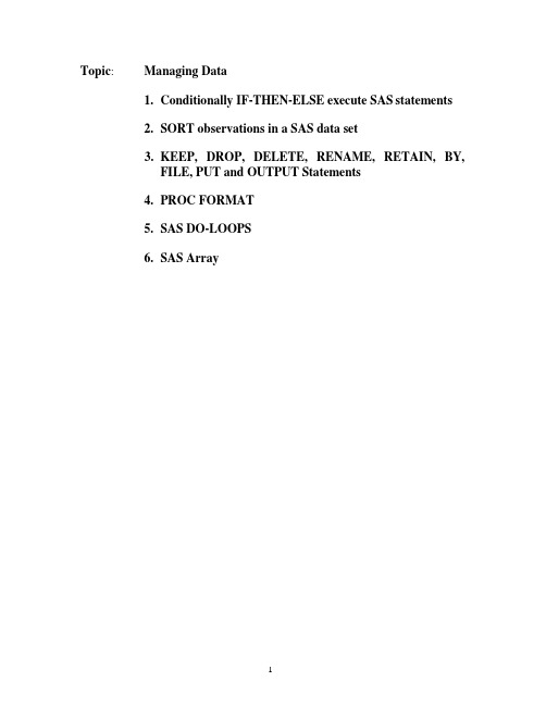
Topic: Managing Data1.Conditionally IF-THEN-ELSE execute SAS statements2.SORT observations in a SAS data set3.KEEP, DROP, DELETE, RENAME, RETAIN, BY,FILE, PUT and OUTPUT Statements4.PROC FORMAT5.SAS DO-LOOPS6.SAS Array1.Conditionally IF-THEN-ELSE execute SAS statementsConditional execution of data step program statements is implemented using theIF/THEN/ELSE statements.Syntax:IF expression THEN statement1;<ELSE statement2;>Observe that IF/THEN and ELSE are two separate SAS statements. Each time the IF statement is executed the expression following the IF is evaluated. When the expression is true for the observation, the statement following the THEN is executed. The ELSE statement, which is optional, can be used to control a specific action if the IF condition is false.Or try to fully understand the following statements:The inputs to the IF /ELSE statements areexpression is an expression that is evaluated for being true or false.statement1 is a statement executed when expression is true.statement2 is a statement executed when expression is false.These examples show different ways of specifying the IF-THEN/ELSE statement./*Example: IF-THEN*/data if_01_a;input code @@;cards;1 2 3;data if_01_b;length type $ 8.;set if_01_a;if code=1 then type ='Fix';if code=2 then type ='Variable';if code ^=1 and code ^=2 then type = 'Unknown';label type ='Types of Mortgage Rate';run;/*Example: IF-THEN/ELSE*/data if_01_c;length type $ 8.;set if_01_a;if code=1 then type ='Fix';else if code=2 then type ='Variable';else if code ^=1 and code ^=2 then type = 'Unknown';label type ='Types of Mortgage Rate';run;Let us see how to divide age group?data age_grp;input pat_id age @@;cards;290156 66 299871 68 280256 64 270456 60 262156 58263256 55 266456 53 250656 44 251256 43 257456 47258356 48 244606 42 249456 41 233256 33 237656 37228356 28 222606 22 219856 21;run;data age_grp2;length agegrp $ 5.;set age_grp;if 20<= age < 35 then agegrp = '20-34';else if 35<= age < 50 then agegrp = '35-49';else if 50<= age < 65 then agegrp = '50-64';else if 65 <= age then agegrp = '65+';run;proc freq ;tables agegrp/list;*tables agegrp/out = age_grp3;run;Advice:A better way to write multiple IF statement is to use an ELSE before all but the first IF. The other IF-THEN/ELSE statements would look like this:If then;Else if then;Else if then;…………..;The effect of the ELSE statements is that when any IF statement is true, all the following ELSE statements are skipped. The advantage is to reduce computer time (since all the IF do not have to be tested) and evenly to avoid the following type of error. Would you see what will happen with the statements below?data er;input x @@ ;cards;1 2 3 4 5;run;data er_2;set er;if x=1 then x=5;if x=2 then x=4;if x=4 then x=2;if x=5 then x=1;run;data er_3;set er;if x=1 then x=5;else if x=2 then x=4;else if x=4 then x=2;else if x=5 then x=1;run;/*Example: IF-THEN/DO*/data oss_test;length course $ 8. school $ 4.;input course school score year;cards;English NT 92 1998English NT 94 1999English NT 96 2000English NT 91 2001English NSS 88 1998English NSS 80 1999English NSS 84 2000English NSS 82 2001Math NT 86 1998Math NT 88 1999Math NT 89 2000Math NT 86 2001Math NT 90 2002Math NSS 84 1998Math NSS 88 1999Math NSS 88 2000Math NSS 92 2001Math NSS 89 2002;data oss_test1 ;set oss_test;if course= 'English' then do;if score > 84 then output ;end;run;data oss_test2;set oss_test;if school = 'NT' then do;if course ='Math' then do;if score >86 then output;end;end;run;Earlier you learned to assign values conditionally using IF-THEN/ELSE statements. You can also use SELECT groups in DATA steps to perform conditional processing. A SELECT group contains these statements:Syntax:SELECT <(select-expression)>;WHEN-1 (when-expression-1 <..., when-expression-n>) statement;WHEN-n (when-expression-1 <..., when-expression-n>) statement;<OTHERWISE statement;>END;Example:data sel;input id salary gender job $;cards;1 2800 0 CA2 3100 0 RN3 2698 1 ME4 4550 1 MD5 3895 1 TA;data sel2;length occupation $ 20 Sex $ 7;set sel;select (id);when (1) income=salary*10;when (3,4) income=salary*15;otherwise income=salary*5;end;select(job);when ('CA') occupation="Chartered Accountant";when ('RN') occupation="Registed Nurse";when ('ME') occupation="Mechanic I";when ('MD') occupation="Doctor";otherwise occupation="Other";end;select(gender);when (0) Sex="Female";when (1) Sex="Male";otherwise Sex='Unknown';end;run;2.SORT observations in a SAS data setBasic Concept:2.1.1Sorting Orders for Numeric VariablesFor numeric variables, the smallest-to-largest comparison sequence is1.SAS System missing values (shown as a period or special missing value)2.negative numeric values3.zero4.positive numeric values.data sorting_1;input x @@ ;cards;. 1 0 -2 3;proc sort data =sorting_1;by x;run;order of output: . -2 0 1 3;2.1.2Sorting Orders for Character Variablesdata sorting_2;input area $ @@;cards;toronto London 535 . hamilton;proc sort data =sorting_2;by area;run;Output: ‘blank’ , 535, London, hamilton, toronto2.2What can SORT do?-Specify the input data set-Create an output data set-Specify the output order-Eliminate duplicate observations with common BY values and other options2.3Applications of PROC SORT procedureThe sort procedure sorts observations in a SAS data set by one or more character or numeric variables, either replacing the original data set or creating a new, sorted data set. PROC SORT by itself produces no printed output.2.3.1Observations Sorted by the Values of One VariableIn this example, PROC SORT replaces the original data set, sorted alphabetically by last name, with a data set that is sorted by employee identification number. The statements that produce the output follow:data sorting_3;input Name $ IDnumber;datalines;Arnsbarger 5466Belloit 1988Capshaw 7338Lemeux 4210Pierce 5779Wesley 2092;proc sort ;by idnumber;run;2.3.2Observations Sorted by the Values of Multiple VariablesThe businesses in this example are first sorted by town, then by debt from highest amount to lowest amount, then by account number.DESCENDING option: reverses the sort order for the variable that immediately follows in the statement so that observations are sorted from the largest value to the smallest value.data sorting_4;input company $ 1-23 town $ 24-36 debt accnt_num;datalines;Apex Catering Apex 37.95 9923Bob's Beds Morrisville 119.95 4998Boyd & Sons Accounting Garner 312.49 4762 Deluxe Hardware Garner 467.12 8941 Elway Piano and Organ Garner 65.79 5217 Ice Cream Delight Holly Springs 299.98 2310 Pauline's Antiques Morrisville 302.05 9112 Paul's Pizza Apex 83.00 1019 Peter's Auto Parts Apex 65.79 7288 Strickland Industries Morrisville 657.22 1675 Tina's Pet Shop Apex 37.95 5108 Tim's Burger Stand Holly Springs 119.95 6335 Watson Tabor Travel Apex 37.95 3131 World Wide Electronics Garner 119.95 1122 ; run ;proc sort ;by town descending debt; run ;2.3.3 Create Output Data Set for the Sorted Observationsproc sort data = sorting_4 out = sorting_5;by town descending debt; run ;2.3.4 Eliminate duplicate observations -NODUPKEY optionIn this example, PROC SORT creates an output data set that contains only the first observation of each BY group. The NODUPKEY option removes an observation from the output data set when its BY value is identical to the previous observation's BY value. The resulting report contains one observation for each town where the businesses are located. It automatically eliminates multiple observations where the By variables have the same value.options nodate pageno=1 linesize=80 pagesize=60; data account;input Company $ 1-22 Debt 25-30 AccountNumber 33-36Town $ 39-51;datalines ; Paul's Pizza 83.00 1019 Apex World Wide Electronics 119.95 1122 GarnerStrickland Industries 657.22 1675 Morrisville Ice Cream Delight 299.98 2310 Holly Springs Watson Tabor Travel 37.95 3131 Apex Boyd & Sons Accounting 312.49 4762 Garner Bob's Beds 119.95 4998 Morrisville Tina's Pet Shop 37.95 5108 ApexSprings Peter's Auto Parts 65.79 7288 Apex Deluxe Hardware 467.12 8941 Garner Pauline's Antiques 302.05 9112 Morrisville Apex Catering 37.95 9923 Apex ;proc sort data =account out =towns nodupkey;by town; run ;Elway Piano and Organ 65.79 5217 Garner Tim's Burger Stand 119.95 6335 Hollyproc print data=towns;var town company debt accountnumber;title 'Towns of Customers with Past-Due Accounts';run;-NODUPLICATE /NODUP/NODUPRECS optionIn this example, the NODUPLICATE option removes observations that have duplicate values with BY value.Example:data sorting_6;input pat_id age;cards;290156 66290156 66280256 64280156 64262156 58263256 55;run;proc sort data =sorting_6 noduplicate out = sorting_7;by age ;run;***Nodupkey, nodup, and noduplicate***;data dup;input account_id visit mmddyy10. checking_bal comma9.2 ;datalines;201189 11/11/1998 7,865.28201189 11/28/1998 5,724.02201189 12/08/1998 6,908.98202369 11/11/1998 4,405.18204189 11/28/1998 5,724.02204189 12/05/1998 8,054.32225189 11/28/1998 3,632.85225189 11/28/1998 3,632.85;proc sort data =dup out=dup2 noduplicate ;by account_id;run;proc sort data =dup nodupkey out=dup3;by account_id;run;proc sort data =dup nodup out=dup4;by account_id;run;/* The COMMAw.d format writes numeric values with commas that separate every three digits and a period that separates the decimal fraction.2.3.5DUPOUTspecifies the output data set to which duplicate observations are written.data a;input bank_id deposits city $;datalines;60925 5672 Toronto60925 5672 Toronto61002 5670 Hamilton61009 7500 Toronto;proc sort data=a dupout=b noduprecs;by bank_id;run;Note: The DUPOUT option is effective only when used with the NODUPKEY or NODUPREC options. Without one of these options, the log will show a WARNING message and the DUPOUT data set will be created with 0 records.3.KEEP, DROP, DELETE, RENAME, RETAIN, BY, OUTPUT, PUT, andFile statements3.1KEEP and DROPBasically say, KEEP and DROP are mutually exclusive.Sometimes you do not need to use all of the variables in a data set for further processing. To restrict the variables in an input data set, the data set option keep= can be used with a list of variable names. For example:data account;input Company $ 1-22 Debt 25-30 Account_Number 33-36Town $ 39-51;datalines;Paul's Pizza 83.00 1019 ApexStrickland Industries 657.22 1675 MorrisvilleIce Cream Delight 299.98 2310 Holly SpringsBoyd & Sons Accounting 312.49 4762 GarnerBob's Beds 119.95 4998 Morrisville;data account_new;set account (keep= account_number town);*keep account_number town;run;Advantage: is very efficient, and prevents all the variables from being read for each observation.Sometimes, if you only wanted to remove a few variables from the data set, or control the variables which will be output to a data set, you could use the drop option to specify the variables in a similar fashion. The DROP statement specifies that some variables be excluded from the OUT= data set.How to get the same result from above example with drop statement?Efficient:The DROP and KEEP statement selection is applied before variables are read from the data file, while the DROP= and KEEP= data set option selection is applied after variables are read and as they are written to the OUT= data set. Therefore, using theDROP and KEEP statement instead of the DROP= and KEEP = data set option respectively is much more efficient.3.2DELETEUse the DELETE statement to mark records for deletion in the current output data set. data account;input Company $ 1-22 Debt 25-30 AccountNumber 33-36Town $ 39-51;datalines;Paul's Pizza 83.00 1019 ApexStrickland Industries 657.22 1675 MorrisvilleIce Cream Delight 299.98 2310 Holly SpringsBoyd & Sons Accounting 312.49 4762 GarnerBob's Beds 119.95 4998 Morrisville;data account_new;set account;*delete ;/* deletes the current obs */if debt < 85 then delete ; /* deletes obs where debt<85 */run;3.3RENAME3.3.1Syntax:Rename old-name = new-name;3.3.2Detail: The RENAME statement is used to change the names of variables in the output data sets. Or it allows you to change the names of one or more variables, variables in a list, or a combination of variables and variable lists. The new variable names are written to the output data set only. The new-name is limited to thirty-two characters.3.3.3Comparison•RENAME cannot be used in PROC steps, but the RENAME= data set option can.•The RENAME= data set option allows you to specify the variables you want to rename for each input or output data set. Use it in input data sets to rename variables before processing.•If you use the RENAME= data set option in an output data set, you must continue to use the old variable names in programming statements for the current DATA step. After your output data is created, you can use the new variable names.•The RENAME= data set option in the SET statement renames variables in the input data set. You can use the new names in programming statements for the current DATA step./* rename cannot be used in PROC steps, but rename=dataset optioncan*/;data rena_me;input patient age ht;datalines;005 65 178003 60 170006 55 172;proc means data = rena_me;var age;rename patient= pat_id;run;proc means data = rena_me(rename=(ht=height));/*ht renamed by height*/; var age height;run;/* The RENAME= data set option allows you to specify the variables you want to rename for each input or output data set. Use it in input data sets to rename variables before processing*/;data rena_me(rename=(ht=height));input patient age ht;datalines;005 65 178003 60 170006 55 172;proc means data = rena_me; var age height; run;/*If you use the RENAME= data set option in an output data set, you must continue to use the old variable names in programming statementsfor the current DATA step. After your output data is created, you can use the new variable names. */;data rena_me(rename=(ht=height));input patient age ht;wt=ht*0.8;datalines;005 65 178003 60 170006 55 172;proc means data = rena_me;var age height wt;run;/*The RENAME= data set option in the SET statement renames variables in the input data set. You can use the new names in programmingstatements for the current DATA step. */;data rena_me;input patient age ht;wt=ht*0.8; datalines;005 65 178003 60 170006 55 172;data rena_me4;set rena_me (rename=(ht=height wt=weight));wt2=weight*0.9;*wt2=wt*0.9;/*comparison*/;run;proc print data=rena_me4;run;3.4RETAINThe RETAIN statement•names the variables which should not be set to missing before the next iteration of the data step (the "retained variables")•may give initial values (for first iteration of data step)•non-executable (can be placed anywhere in the data step)Because SAS default behavior is to set all variables to missing each time a new observation is read. Sometimes it is necessary to “remember” the value of a variable from previous observation. Retained variables are important especially in working with grouped observations. First, we'll examine the concept with a simple example.Example:data alpha;input a b c;retain runtot 0; /*runtot will keep a running total of a, b, c */ runtot=runtot + (a+b+c);cards;2 4 63 1 50 7 98 5 4;run;proc print;run;What is the output?How a retained variable behaves during data step executionTo understand the values of the retained variable RUNTOT on the output observations, picture shown using data step execution as follows.Before input a b c; is executed the first time:A B C RUNTOT| | | || | | | 0| | | |After input a b c; is executed the first time:A B C RUNTOT| | | | || 2 | 4 | 6 | 0 || | | | |After runtot=runtot + (a+b+c); is executed the first time:A B C RUNTOT| | | | || 2 | 4 | 6 | 12| 1st obs output: A B C RUNTOT| | | | | 2 4 6 12After input a b c; is executed the second time:A B C RUNTOT| | | | || 3 | 1 | 5 | 12|| | | | |After runtot=runtot + (a+b+c); is executed the second time:A B C RUNTOT| | | | || 3 | 1 | 5 | 21| 2nd obs output: A B C RUNTOT| | | | | 3 1 5 213.5By StatementOrders the output according to the BY groups. By-group processing refers to the use of a BY statement in a DATA step, which permits identification of the first- and last- occurring record for each of the specified BY variables. Two dichotomous (1/0) variables are automatically created for each variable specified in the BY statement when using SET, MERGE, or UPDATE, FIRST.varname and LAST.varname, where varname is the name of the BY variable(s). By creating these variables, a number of various calculations are possible, such as obtaining a count of records for each unique identifier. You can only use one BY statement in each PROC step.In the DATA step, SAS identifies the beginning and end of each BY group by creating two temporary variables for each BY variable: FIRST.variable and LAST.variable.These temporary variables are available for DATA step programming but are not added to the output data set. Their values indicate whether an observation is•the first one in a BY group•the last one in a BY group•neither the first nor the last one in a BY group•both first and last, as is the case when there is only one observation in a BY group.You can take actions conditionally, based on whether you are processing the first or the last observation of a BY group. For the first record in a BY group, the value of theFIRST.varname1 is set to 1, with all other records in the BY group set to 0. For the last record in a BY group, the value of the LAST.varname1 is set to 1, with all other records set to 0. FIRST. and LAST. variables are not kept in the newly created data set since they are usually just used for subsequent processing. Their value can be assigned, however, to other variables.data hosp;input PHIN @@ ;cards;562737 563850 563961 565858 566739 568729 568729 568729 569961 660861;PROC SORT data=hosp;BY phin;RUN;DATA dup;SET hosp;BY phin; (1)firstfl=FIRST.phin; (2)lastfl=LAST.phin; (3)RUN;(1)Set the data by PHIN (already previously sorted by this variable) in order to create FIRST.PHIN and LAST.PHIN.(2)Create a new variable called FIRSTFL and assign it a value of 1 for everyFIRST.PHIN=1 encountered.(3)Create a new variable called LASTFL and assign it a value of 1 for everyLAST.PHIN=1 encountered.In the above example, the person with PHIN 568729 has 3 record s (observations 6-8). For the first record (#6), FIRSTFL is set to 1, indicating that it is the first record for that person and all other records for that PHIN show FIRSTFL values set to 0. For the third and last record, LASTFL is set to 1, indicating that it is the last record for that person and all other records show LASTFL values set to 0.DATA ONE;INPUT SUBJECT SCORE @@;DATALINES;1 112 213 31 1 124 41 1 13 2 22 4 42 4 43;/*Using FIRST. and LAST. Variables to Count Observations per Subject*/; PROC SORT DATA=ONE;BY SUBJECT;RUN;DATA COUNT;SET ONE;BY SUBJECT;IF FIRST.SUBJECT = 1 THEN NUMBER = 0;NUMBER + 1;IF LAST.SUBJECT = 1 THEN OUTPUT;KEEP SUBJECT NUMBER;RUN;PROC PRINT DATA=COUNT;TITLE "Counting Observations per Subject";RUN;PROC FREQ DATA=ONE NOPRINT;TABLES SUBJECT/OUT=CNT; RUN;Example: /* to keep first/last observation '*/; data clean;input patno gender hr temp visit $dx ae sbp dbp; datalines;0235 1 75 92.6 052398 2 0 120 650235 1 75 92.6 052398 2 0 120 650256 1 80 92.1 052498 4 1 110 700367 2 78 91.7 052398 3 1 110 650235 . 75 92.6 053098 2 0 118 700256 1 78 91.8 053198 4 1 110 730235 0 . 92.6 . 8 1 120 700367 0398 21809692.096.7.060298. 010 21201307585;* to check multiple observations;proc sort data = clean;by patno;run;data multi2 a b;set clean;by patno;*if first.patno;*if last.patno;if first.patno then output a;if last.patno then output b;run;proc print data = multi2;*title 'First observation to keep';title ' Last observation to keep';run;/*count*/;data multi4;set clean;by patno;if first.patno then do;count=0;end;retain count;count =count +1;if last.patno then output;run;proc print data=multi4;run;3.6OUTPUTSyntax:OUTPUT out=SAS-data-set <DATA=SAS-data-set>; Example:/*SAS-data-set*/;data out_01;input id age;datalines;001 78002 76003 77004 70005 73;proc means data =out_01 nway sum;var age;output out = out_02(drop= _freq_ _type_)/*new dataset*/mean = m_agesum = s_age;run;/* DATA=SAS-data-set*/;data out_03 out_04 out_05;set out_01;if id=001 then output out_03;else if id=002 then output out_04;else if id=003 then output out_05;run;3.7PUTThe PUT statement is used to print or store information in a specified format. It is also useful for generating data files which are to be used later by other programs. Put writes lines to the SAS log, to the SAS procedure output file, or to an external file that is specified in the most recent FILE statement. It is valid in a DATA step.You can use a PUT statement to specify a character string to identify your message in the log. The character string must be enclosed in quotation marks.put 'NOTE: PUT is a statement';Note that when you specify a variable in the PUT statement, only its value is written to the log. To write both the variable name and its value in the log, add an equal sign (=) to the variable name.put 'Invalid value:' KEYID= ;You can use the '@' to specify the initial print position (column) of the output a variable. SAS enables you to specify the beginning column number for the data and its format. For example, you could substitute the following statement for the PUT statement in the second DATA _NULL_ in the above example:PUT @6 Y 11.2 @18 X1 11.2 @30 X2 11.2@42 predict 11.2 @54 residual 11.2 ;In the example: reporting format, the HEADER=HEADING option on the FILE statement tells SAS to execute the PUT statements which follow the label HEADING(labels have a ':' after them) and then continue with the printing of the lines. This allows a heading to print at the top of each page.DATA report;INPUT ssn 1-9 grossinc 10-20 taxrate 21-23 ;FILE PRINT HEADER=heading NOTITLES;netinc = grossinc - (grossinc*taxrate);PUT ssn @30 grossinc @50 netinc; RETURN;heading:PUT _PAGE_ 'LISTING OF INCOMES' / ;PUT @1 'SOCIAL SECURITY NUMBER' @30 'GROSS INCOME' @50 'NET INCOME'; RETURN;CARDS;564981234 45689 0.15;data club1;input idno name $ startwght date : date7.;put name;put idno 1-3 name 5-10 ;datalines;032 David 180 25nov99049 Amelia 145 25nov99219 Alan 210 12nov99;Moving the Pointer within a Pageput @15 name;3.8FILEIt identifies an external file that the DATA step uses to write output from a PUT statement. SAS FILE and PUT statements work very well for creating flat files. The FILE statement specifies the output file where the data will be written. If you want the results in your LISTING file, use the file reference name PRINT on the FILE statement as illustrated below:A typical program might look like the following:data club1;input idno name $ startwght date : date7.;file 'c:\aa.txt';file print;put name;datalines;032 David 180 25nov99049 Amelia 145 25nov99219 Alan 210 12nov99;The PUT statement in the example above uses a format list where the variable is specified and is followed by the desired format.4.PROC FORMAT4.1Introduction: Data values are inadequate to display in an output destination. The data values are usually coded values -- '0' for 'yes' or ‘survival’ and '1' for 'no' or ‘death’, et al.These values are not clear to casual users who inspect output. SAS institute provides numerous means for changing the appearance of data values when displayed in an output destination. A format can be applied as needed. These formats go a long way in satisfying the usual needs for displaying data in a more customary and user-friendly manner.4.2 PROC FORMAT allows the programmer to create user-defined formats to meet programming needs. Some aspects of Proc Format and the formats they create include1. formats are applied to a variable, usually in a Format statement2. applying a format to a variable does not change the values in the data set3. formats determine only how the data is presented in the output destinationWe discuss PROC FORMAT concentrating on the value statement.The Value Statement1. is used only in Proc Format2. identifies the name of the format being created3. identifies the association between the data values and output labels4. is used to create formats for both character and numeric type variables5. recodes dataWhen naming a format, follow these rules:1. formats are limited to names of eight characters or fewer2. format names should use letters or underscore only; do not use numbers3. character formats all begin with a dollar sign ($) which counts as one of thecharacters in the name4. do not name a format the same name as a format supplied by SAS Institute.5. if a format is given a name longer than eight characters, SAS will use onlythe first eight characters when assigning the name.6. the format definition ends with the “ ; “ on a new line. This is just my preference.7. do not end with numbers and dot.4.3 Examplesdata format_01;input name $ 1-19 id_num salary dollar8.0 site $ ; datalines ;Capalleti, Jimmy 2355 $34,072 BR1Chen, Len 5889 $33,771 BR2Davis, Brad 3878 $31,509 BR3Martinez, Maria 3985 $78,980 US1Orfali, Philip 0740 $80,648 US2Smith, Robert 5162 $64,561 INCORRECT CODE;proc format ;value $city 'BR1'='Birmingham UK''BR2'='Plymouth UK''BR3'='York UK''US1'='Denver USA''US2'='Miami USA'Other='INCORRECT CODE';Sorrell, Joseph Zook, Carla 4421 $62,403 US17385 $37,010 BR3。
整理的SAS笔记
第一章sas是什么1.SAS系统是一个模块化的集成软件系统;——数据处理和统计领域的国际标准软件;——世界领先的数据分析和信息系统;SAS系统广泛应用于金融、医疗、运输、通迅、政府、科研和教育等领域;SAS含义Statistical Analysis System2.SAS系统的主要四大功能数据访问数据管理数据分析数据呈现3.SAS系统对50多种数据源提供了引擎,如:DB2 和Oracle-------------------------------------------第二章开始sas程序的讲解1.sas程序的介绍有两种程序步组成,数据步和过程步,每个步通常有若干个SAS语句组成;数据步:以data语句开始,用于创建和处理SAS数据集;过程步:以proc语句开始,主要用户处理SAS数据集;2.SAS数据集通常分为两个部分:描述部分(包含数据属性的信息)和数据部分(包含数值);数据集的列称为变量(Variable),行称为观测(Observation)。
查看数据集的描述部分:proc contents data=sas_data_set;run;查看数据集的数据部分:proc print data=sas_data_set;run;4.SAS变量的类型*字符型变量(Character Variable )(1-32767字节),均以字母、下划线开头;字符型变量的缺省数据用空格表示;*数值型变量(Numerical Variable )默认为8个字节的长度,数值型变量的缺省数据用点(.)表示;5.变量的命名规范:1-32个字符长度,不区分大小写,以下划线或字母开头-------------------------------------------第三章sas数据仓库1.每次SAS启动都自动生成三个库标记:WORK、SASUSER和SASHELP;2.库的分类永久性库:sasuser、sashelp、自定义的库临时性库:只有一个,名为WORK,可以省略库标记;每次启动SAS自动生成,结束SAS后库中的数据被自动删除;用libname指定库标记,如:libname temp“e:\temp\data”;3.使用关键词_ALL_列出数据仓库中所有的sas文件,使用NODS option来禁止对数据集的描述PROC CONTENTS DATA=libref._ALL_ NODS;RUN;注意:NODS选项只能和_ALL_一起联用-------------------------------------------第四章数据列表报表1.print过程语法格式:proc print data=SAS数据集noobs;var 分析变量1 分析变量2 ... 分析变量n;where 表达式;sum 求和变量;run;Noobs选项:在PRINT过程中可以用NOOBS选项去掉OBS列;VAR语句:控制变量的出现与否以及出现的顺序;WHERE语句:控制哪些观测将出现在报表中;它的表达式主要是操作数和操作符,SUM语句:计算变量的总合;2.观测的排序和分组§(sort)和(by)对数据进行分组并求每组小计,用PRINT过程的BY语句,但必须先对相应的变量进行排序;如:proc sort data=temp.empdata out=temp.empdata2;By JobCode;Run;proc print data=temp.empdata;by JobCode;sum Salary;pageby JobCode; /*使产生的报表按组分页*/run;-------------------------------------------第五章:输出1.标题和脚注:在所有的SAS报告中都可以加标题(Title)和脚注(Footnote):语法格式:TITLEn ‘text’;FOOTNOTEn ‘text’;特点:n 的取值范围是1-10;标题出现在每页的顶部;脚注出现在每页的底部;如果没有定义标题,缺省的标题是:“The SAS System”;如果没有脚注就不出现;没有n的标题和脚注就是:TITLE1、FOOTNOTE1;定义的标题和脚注一直有效,知道另一个语句被执行;带n的标题或脚注被执行后,替代了原先具有同样号码的标题和脚注;带n的标题或脚注被执行后,取消了更大号码的标题和脚注;BEL语句:产生用户化和容易阅读的表头:如:label 变量1=’标签’变量2=’标签’;属性:是最大长度为256个字符串;注意:在PRINT过程中必须用PRINT语句中的LABEL或SPLIT=选项才能被显示;在过程步中定义只在该过程中有效;在数据步中定义就被存在数据集的描述部分与数据集一直有效;3.format的使用分类:系统format和用户自定义format4.用户自定义format的使用format变量的语法格式:<$>format<w>.<d>在VALUE语句中,格式可以赋予为:A.单个数字:如:Proc format;Value gender 1=’Female’2=’Male’Other=’Miscoded’;Run;B.某数字范围:如:Proc format;Value boadfmt low-49=’Below’50-99=’Average’100-high=’Above Average’;Run;C.字符或字符串:如:Proc format;Value $grade ‘A’=’GOOD’‘B’-‘D’=’PAID’‘I’,’W’=’POOR’‘PILOT’=’pilot’Other=’Miscoded’;Run;format的使用步骤:第一步:用户创建formatPROC FORMAT;VALUE format-name range1='label 'range2='label '. . . ;RUN;第二步:应用所创建的formatproc print data=ia.empdata;format [$]varialble-name format-name;run;5.使用ODS创建html报表(利用ODS将SAS输出结果生成HTML格式文件)ODS--Output Delivery System语法格式:ODS HTML FILE='HTML-file-specification' <options>; 产生输出的sas代码ODS HTML CLOSE;第六章创建sas数据集1.列输入(column input)*此模式读入外部原始数据文件,适应文件为:数据固定在某些列中;数据只包含标准的数字和字符;*过程:a.开始一个数据步,并给数据步命名b.用infile指明原始数据的存放位置c.用input指明怎样读取原始数据*格式:data 库名.数据集名;infile '文件名(路径)' <选项>;input 变量名<$> 起始列-结束列;($用在变量是字符型) run;2.格式输入(formatted input)*适合用格式输入的外部原始数据文件数据是固定列;但含有标准或者不标准字符以及数字的文件;*语法格式:data SAS数据集;Infile ‘外部原始文件’;INPUT 指针控制变量名<$> 格式名;($表示字符型变量)Run;*指针的控制:@n 移动指针到第几列(绝对位置)+n 把指针移动几个位置(相对位置)3.输入格式informat<$>informat-namew.<d>说明:$ 如果是字符型,使用$informat-name是输入格式的格式名w 是变量总长度. 句点是必修的分隔符,不能缺少d 如果是数值型的话, d指定了小数位的长度4.分配变量属性变量的临时属性和永久属性:PROC步可赋予临时属性:其中的标签只在该步显示时有,并没存在数据集里;如:proc print data=temp.dfwlax label;Label Dest=’Destination’FirstClass=’First Class Passengers’;Run;DATA步可赋予永久属性:其中的标签被存在数据的描述部分,与数据集一起存在;如: data temp.dfwlax;Infile ‘‘c:\course\tempdata.dat’;Input @12 Dest $3. @15 FirstClass $3. ;Label Dest=’Destination’FirstClass=’First Class Passengers’;Run;---------------------------------------------------------------------------------------第七章数据步程序设计1.读sas数据集以及创建变量用DATA步产生SAS数据集的三种方法:A.数据在作业流中:DATA 语句;INPUT 语句;CARDS;数据行;;RUN;B.数据在磁盘上:DATA 语句;INFILE 语句;INPUT 语句;RUN;C.数据来自其它SAS数据集:DATA 语句;SET / MERGE / UPDATE / MODIFY语句;<DATA步中的其它SAS语句>;RUN;2.用已有的数据集创建另一个数据集[set的使用]DATA 新的数据集名;SET input-SAS-data-set;<additional SAS statements>RUN;3.sas操作符和函数的使用语法格式:function-name(argument1,argument2, . . .)函数:sum(argument1,argument2, . . .);TODAY();MDY(month,day,year);QTR(SAS-date);MONTH(SAS-date);WEEKDAY(SAS-date);4.有条件的程序语法结构:简单if语句IF expression THEN statement;ELSE statement;复杂if语句IF expression THEN DO;executable statementsEND;ELSE DO;executable statementsEND;设置变量长度LENGTH variable(s) $ length;取数据集子集a.WHERE语句b.DELETE语句IF expression THEN DELETE;c.子集IF语句IF expression;使用sas日期常数格式:'ddMMMyyyy'd例如:(example: '14dec2000'd)说明:'d是必须的,用来把引号里的字符串转换成sas日期-------------------------------------------------------------------------------------------- 第八章数据拼接1.使用set连接sas数据集语法格式:DATA SAS-data-set ;SET SAS-data-set1 SAS-data-set2 . . . ;<additional SAS statements>RUN;set中变量重命名语法格式:SAS-data-set(RENAME=(old-name-1=new-name-1old-name-2=new-name-2 ...old-name-n=new-name-n));交叉sas数据集,使用by语句BY语句:使用BY语句可使生成的数据集按某变量排序,但输入数据集必先按该变量排序过;语法格式:DATA SAS-data-set;SET SAS-data-set1 SAS-data-set2 . . . ;BY BY-variable;<other SAS statements>RUN;2.MERGE sas数据集(必先排序)MERGE语法格式:DATA SAS-data-set;MERGE SAS-data-sets;BY BY-variable(s);<additional SAS statements>RUN;IN= 选项格式:SAS-data-set(IN=variable)解释:一个临时的数字类型的变量,其值为0或者1IN选项,当读入多个SAS数据集时,用IN选项可确定本观测来自哪个数据集;variable=0表示观测不是来自本数据集variable=1表示观测是来自本数据集-------------------------------------------第九章制作汇总报表1.基本的汇总报表(freq、mean)freq报表默认的情况下:分析每一个变量,显示出每一个数据值,计算出数字类型的每列的百分比,指出每一个变量有多少条观测中有缺失值用此过程一般有两个目的:1:描述过程:产生频数表和交叉表,可简洁的描述数据;2:统计过程:产生各种统计量(频数、百分比),分析变量间关系;使用:A.单项频数表:PROC FREQ DATA=SAS数据集;TABLES 变量;RUN;B.双向交叉表:PROC FREQ DATA=SAS数据集;TABLES 行变量*列变量;RUN;C.n向交叉表:PROC FREQ DATA=SAS数据集;TABLES a*b*c*d;RUN;如果要一张三向(或n向)交叉表,只要在TABELS语句中用星号将3个(或n个)变量名连接起来。
SAS备课笔记_第三部分_描述统计分析
目录一、描述性分析的分类_______________________________________________ 2(一)数据分类_________________________________________________________ 2(二)定量数据的描述性分析_____________________________________________ 3(三)定性数据的描述性分析_____________________________________________ 4(四)例题的数据说明___________________________________________________ 4二、SAS实现-程序___________________________________________________ 5(一)means过程_______________________________________________________ 5(二)summary过程_____________________________________________________ 7(三)univariate过程 ____________________________________________________ 9(四)tabulat过程______________________________________________________ 13(五)四个过程的比较__________________________________________________ 14(六)freq过程________________________________________________________ 14(七)capability过程___________________________________________________ 16(八)gchart过程 ______________________________________________________ 18(九)gplot过程 _______________________________________________________ 20三、SAS实现-图形界面______________________________________________ 21(一)SAS/ASSIST _____________________________________________________ 21(二)SAS/ANALYST(分析家)_________________________________________ 22(三)SAS/INSIGHT(交互式数据分析)__________________________________ 23(四)三种方法比较____________________________________________________ 23第三部分数据的描述性分析描述性统计分析(Descriptive Statistics )是基础统计分析(Elementary Statistics),是综合统计分析(Summary Statistics)。
SAS备课笔记_简单线性回归、多元线性回归
回归分析-简单线性回归、多元线性回归比较:方差分析是处理试验数据的一类统计方法。
这类统计方法的特点是所考察的指标(因变量)Y 是测量得到的数值变量(连续变量),而影响指标的因子(自变量)水平是试验者安排的几个不同值(称这种因子为分类变量或离散变量)。
试验的目的是找出影响指标的主要因子及水平。
在实际问题中,还经常遇到这样一些数据,它们不是有意安排的试验得到的数据,而是对生产过程测量记录下来的数据。
对它们进行分析,目的是想找出对我们所关心的指标(因变量)Y 有影响为因素(也称自变量或回归变量)m x x x ,......,,21,并建立用m x x x ,......,,21预报Y 的经验公式。
对于现实世界,不仅要知其然,而且要知其所以然。
顾客对商品和服务的反映对于商家是至关重要的,但是仅仅有满意顾客的比例是不够的,商家希望了解什么是影响顾客观点的因素,以及这些因素是如何起作用的。
类似地,医疗卫生部门不能仅仅知道某流行病的发病率,而且想知道什么变量影响发病率,如何影响发病率的。
发现变量之间的统计关系,并且用此规律来帮助我们进行决策才是统计实践的最终目的。
一般来说,统计可以根据目前所拥有的信息(数据)来建立人们所关心的变量和其他有关变量的关系。
这种关系一般称为模型(model )。
假如用Y 表示感兴趣的变量,用X 表示其他可能与Y 有关的变量(x 也可能是若干变量组成的向量)。
则所需要的是建立一个函数关系Y=f(X)。
这里Y 称为因变量或响应变量(dependent variable, response variable ),而X 称为自变量,也称为解释变量或协变量(independent variable ,explanatory variable, covariate)。
建立这种关系的过程就叫做回归(regression )。
一旦建立了回归模型,除了对各种变量的关系有了进一步的定量理解之外,还可以利用该模型(函数或关系式)通过自变量对因变量做预测(prediction )。
SAS知识串讲(三)(学生版-A3印刷) _7231b4937209412990b9913c0ffcaf6c.PDF
此以外 N 最小为( )。
A.625
B.676
C.729
D.900
23.A 和 B 都是奇数,C 和 D 都是偶数,且它们互不相等,又 1 1 1 1 ,则 C+D 的最小值为(
ABC D
A.14
B.16
C.18
D.20
)。
24.一辆汽车在公路上匀速行驶,司机看见里程碑上的数字是一个两位数(用 AB 表示),马上看看手表记下时间,一 个小时以后,再看看里程碑,上面仍然是一个两位数,不过恰好是第一个两位数颠倒了顺序(用 BA 表示).再过一 小时,里程碑上是三位数,又恰好是第一个两位数中间加了个零(用 A0B 表示),请问车速是多少?三个里程碑上的 数字各是什么?
2018 武汉 SAS·知识串讲
内部资料
世奥赛赛前冲刺(三)
计数与数论 一、真相到底几种可能
1.荷兰花甲蒙德里安(1872~1944)被称为抽象美术的先驱者。下面这幅图就是蒙德里安的作品,他只采用水平和垂 直两种线条,以此构成各种不同的正方形和长方形,构成简单而又复杂的图形,以使用红、黄、蓝 三原色或黑、白、灰来表示色彩的纯净。 萌萌看着蒙德里安的作品,决心自己也要创作一幅抽象美术作品。打算利用直线和红色的、黄色的 颜料按照下面规则完成作品。 (1)在纸上,遵照下面的规律,按照 2 条横线 1 条竖线这样的顺序一直画。
15.某自然数减去 39 是一个完全平方数,减去 144 也是一个完全平方数,求此自然数为( )。
A.160,208,400,2848 B.55,160,208,400
C.160,208,439,2236
D.160,208,400,1264
16.在自然数中,12=1,22=4,32=9,……数 1,4,9,……称为完全平方数,若自然数 N 121212(1m2018) 是一
- 1、下载文档前请自行甄别文档内容的完整性,平台不提供额外的编辑、内容补充、找答案等附加服务。
- 2、"仅部分预览"的文档,不可在线预览部分如存在完整性等问题,可反馈申请退款(可完整预览的文档不适用该条件!)。
- 3、如文档侵犯您的权益,请联系客服反馈,我们会尽快为您处理(人工客服工作时间:9:00-18:30)。
NOTE: 从数据集 DATA.HF000012 读取了 124 个观测。
WHERE (date>='01AUG2006'D) and (tvolume>=100000) and (tprice>0); NOTE: 数据集 EX.BLOCK 有 124 个观测和 31 个变量。
NOTE: "DATA 语句"所用时间(总处理时间):
实际时间 0.15 秒
CPU 时间 0.10 秒
可见 if语句是先读取数据然后再选择符合要求的观测而where语句则是直接读入满足条件的观测〓
★作业 3.2 先用select语句再用 where语句〓
★作业3.4〓
★第一题〓
d d a a t t a a ex.hm3_4_1(keep=dat
e prevclpr oppr clpr color fluctuate); informat color $6.;★老师加的默认长度是多少呢?〓
se t data.stk000001;
fluctuate=(clpr-prevclpr)/prevclpr;★可以放在if语句后〓
if oppr>clpr then color='red';
if oppr<clpr then color='green';
run;
★if还可以写成这样:
proc sort data=ex.blocktrade;★老师的做法接在第一步后〓by date;
run;
d d a a t t a a num;
set ex.blocktrade;
by date;
if first.date then num=0;
num+1;
if last.date;
keep date num;
run;
merge ex.blocktrade num(in=id); by date;
if id=1;
run;
do n=1to50;
t=t*2*n;
output;
end;
run;
★作业3.5〓
★第一题〓
★第二题〓
d d a a t t a a ex.derivative;
array s(0:20) s_0-s_20;
do i=1to1000;
s_0=17.18;
do j=0to19;
s(j+1)=s(j)*exp((0.03-0.15**2/2)*0.05+0.15*sqrt(0.05)*rannor(0)); end;
output;
end;
drop i j;
run;
d d a a t t a a ex.average_derivative;
set ex.derivative;
if min(of s_1-s_20)<15then value=(18- min(of s_1-s_20))*exp(-0.03*1);★这里不确定value中所用的t值是否应为1〓
if min(of s_1-s_20)>=15then value=0;
run;
★作业3.5〓★老师的答案〓
★a)〓
d d a a t t a a ex.ex3_5_1;
array S(0:20) S_0-S_20;
do i=1to1000;
S_0=17.18;
do j=0to19;
S(j+1)=S(j)*exp((0.03-0.15**2/2)*0.1+0.15*sqrt(0.05)*rannor(0));
end;
output;
end;
drop i j;
run;
run;
★b)〓
d d a a t t a a ex3_5_3;
set ex3_5_1;
array S(0:20) S_0-S_20;
do j=0to20;
if S(j)<=15then leave;
end;
if j=21then value=0;
else do;
payoff=18-S(j);
value=payoff*exp(-0.03*j*0.05);
end;
drop j payoff;
run;
(注:可编辑下载,若有不当之处,请指正,谢谢!)。