维纳滤波 Wiener Filtering
第八章 维纳滤波
第八章 维纳滤波
rpp (0) rpp (1) rpp ( N ) rpp ( N 1) rpp ( N 1) h(1) 0 h ( N ) rpp (0) 0
求解此式,可得到最小平方反滤波的滤波因子 h(n) 。然而求 h(n) 值是根据 rpp(i),为了计算rpp(i)就得确切知道干扰系统的冲激响应p(n),这是一个难题。 在许多情况下,希望由x(n)=p(n)*s(n)以及对p(n)的若干特征来寻求p(n)的估计 值。下面给出一种由x(n)计算rpp(i)的近似方法。
中原工学院
机电学院
x(n) r k s(n kn 0 )
k 0
此式表达了回声干扰信号的数学模型,根据此式,可求得传输函数(或称 为由于鸣震效应而产生的反射函数) 1 n
X ( z) 1 k kn0 反射函数 P( z ) r z S ( z ) k 0 1 rz n0
第一节
一、最小平方滤波
维纳滤波
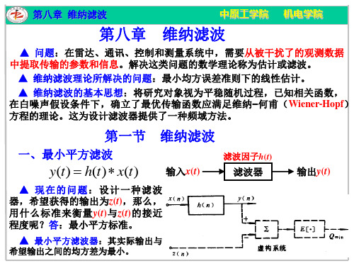
滤波因子h(t)
y (t ) h(t ) x(t )
▲ 现在的问题:设计一种滤波 器,希望获得的输出为z(t),那么, 用什么标准来衡量 y(t) 与 z(t) 的接近 程度呢?答:最小平方标准。 ▲ 最小平方滤波器:其实际输出与
希望输出之间的均方差为最小。
输入x(t)
第2章 维纳滤波讲解
J min (w R 1p) T R ( w R 1p) J min (w w o ) T R (w w o )
(该式表明最佳权向量与最小均方误差的对应关系)
为使误差性能曲面的表达式简单化,定义权偏差向量为
T , w1 ,, w w w w o w0 M 1
结论:维纳滤波器所得最小均方误差等于期望响应的方差与滤波器输出方差的差值。
6
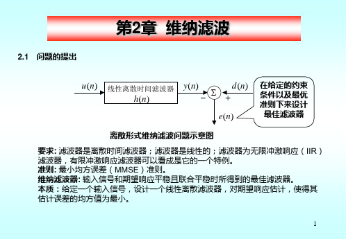
第2章 维纳滤波
2.4 横向滤波器的维纳解 2.4.1 横向滤波器的维纳-霍夫方程及其解
u (n)
u ( n 1)
z w0
1
z
1
u (n M 2)
z
1
u ( n M 1)
w1
wM 2
wM 1
u (n) ,当前输出 y (n) ,期望响应为 d (n) 滤波器的当前输入值: 重写维纳-霍夫方程
M 1 i 0
w
oi
r (i k ) p(k ) k 0,1,2,
定义横向滤波器的抽头输入 u(n), u(n 1),, u(n M 1) 的相关矩阵为R,则
p E[u(n)d (n)] [ p(0), p(1),, p(1 M )]T
则横向滤波器的维纳-霍夫方程式的矩阵表示形式为 Rwo p ,即维纳解为 w o R 1p 式中: w o [wo,0 , wo,1 ,, wo,M 1 ]T 是横向滤波器最优抽头权向量。
J J J J J , ,, 0 w w0 w1 wM 1
T
而 故可推出
J 2Rw(n) 2p
Rwo p ,与维纳-霍夫方程一致。
10
外文翻译---自适应维纳滤波方法的语音增强
附录ADAPTIVE WIENER FILTERING APPROACH FOR SPEECHENHANCEMENTM. A. Abd El-Fattah*, M. I. Dessouky , S. M. Diab and F. E. Abd El-samie #Department of Electronics and Electrical communications, Faculty of ElectronicEngineering Menoufia University, Menouf, EgyptE-mails:************************,#*********************ABSTRACTThis paper proposes the application of the Wiener filter in an adaptive manner inspeech enhancement. The proposed adaptive Wiener filter depends on the adaptation of the filter transfer function from sample to sample based on the speech signal statistics(meanand variance). The adaptive Wiener filter is implemented in time domain rather than infrequency domain to accommodate for the varying nature of the speech signal. Theproposed method is compared to the traditional Wiener filter and spectral subtractionmethods and the results reveal its superiority.Keywords: Speech Enhancement, Spectral Subtraction, Adaptive Wiener Filter1 INTRODUCTIONSpeech enhancement is one of the most important topics in speech signal processing.Several techniques have been proposed for this purpose like the spectral subtraction approach, the signal subspace approach, adaptive noise canceling and the iterative Wiener filter[1-5] . The performances of these techniques depend on quality andintelligibility of the processed speech signal. The improvement of the speech signal-tonoise ratio (SNR) is the target of most techniques.Spectral subtraction is the earliest method for enhancing speech degraded by additive noise[1]. This technique estimates the spectrum of the clean(noise-free) signal by the subtraction of the estimated noise magnitude spectrum from the noisy signal magnitude spectrum while keeping the phase spectrum of the noisy signal. The drawback of this technique is the residual noise.Another technique is a signal subspace approach [3]. It is used for enhancing a speech signal degraded by uncorrelated additive noise or colored noise [6,7]. The idea of this algorithm is based on the fact that the vector space of the noisy signal can be decomposed into a signal plus noise subspace and an orthogonal noise subspace.Processing is performed on the vectors in the signal plus noise subspace only, while the noise subspace is removed first. Decomposition of the vector space of the noisy signal is performed by applying an eigenvalue or singular value decomposition or by applying the Karhunen-Loeve transform (KLT)[8]. Mi. et. al. have proposed the signal / noise KLT based approach for colored noise removal[9]. The idea of this approach is that noisy speech frames are classified into speech-dominated frames and noise-dominated frames. In the speech-dominated frames, the signal KLT matrix is used and in the noise-dominated frames, the noise KLT matrix is used.In this paper, we present a new technique to improve the signal-to-noise ratio in the enhanced speech signal by using an adaptive implementation of the Wiener filter. This implementation is performed in time domain to accommodate for the varying nature of the signal.The paper is organized as follows: in section II, a review of the spectral subtraction technique is presented. In section III, the traditional Wiener filter in frequency domain is revisited. Section IV, proposes the adaptive Wiener filtering approach for speech enhancement. In section V, a comparative study between the proposed adaptive Wiener filter, the Wiener filter in frequency domain and the spectral subtraction approach ispresented.2 SPECTRAL SUBTRACTIONSpectral subtraction can be categorized as a non -parametric approach, which simply needs an estimate of the noise spectrum. It is assume that there is an estimate of the noise spectrum that is typically estimated during periods of speaker silence. Let x (n ) be a noisy speech signal :x (n ) = s (n ) + v (n ) (1) where s (n ) is the clean (the noise -free) signal, and v (n ) is the white gaussian noise. Assume that the noise and the clean signals are uncorrelated. By applying the spectral subtraction approach that estimates the short term magnitude spectrum of the noise -freesignal ()ωS by subtraction of the estimated noise magnitude spectrum )(ˆωVfrom the noisy signal magnitude spectrum ()ωX It is sufficient to use the noisy signal phase spectrum as an estimate of the clean speech phase spectrum,[10]:()()()()()()ωωωωX j N X S ∠-=exp ˆˆ (2) The estimated time -domain speech signal is obtained as the inverse Fourier transform of ()ωSˆ. Another way to recover a clean signal s (n ) from the noisy signal x(n ) using the spectral subtraction approach is performed by assuming that there is an the estimate of the power spectrum of the noise Pv ( ω) , that is obtained by averaging over multiple frames of a known noise segment. An estimate of the clean signal short -time squared magnitude spectrum can be obtained as follow [8]:()()()()()⎪⎩⎪⎨⎧≥--=otherwisev P X if v P X S ,00ˆ,ˆˆ222ωωωωω (3) It is possible combine this magnitude spectrum estimate with the measured phase and then get the Short Time Fourier Transform (STFT) estimate as follows:()()()ωωωX j e S S∠=ˆˆ (4) A noise -free signal estimate can then be obtained with the inverse Fourier transform. This noise reduction method is a specific case of the general technique given by Weiss, et al. and extended by Berouti , et al.[2,12].The spectral subtraction approach can be viewed as a filtering operation where high SNR regions of the measured spectrum are attenuated less than low SNR regions. This formulation can be given in terms of the SNR defined as:()()ωωv P X SNR ˆ2= (5) Thus, equation (3) can be rewritten as:()()()()()1222211ˆˆ-⎥⎦⎤⎢⎣⎡+≈-=SNR X X v P X S ωωωωω (6) An important property of noise suppression using spectral subtraction is that the attenuation characteristics change with the length of the analysis window. A common problem for using spectral subtr action is the musicality that results from the rapid coming and going of waves over successive frames [13].3 WIENER FILTER IN FREQUNCY DOMAINThe Wiener filter is a popular technique that has been used in many signal enhancement methods. The basic principle of the Wiener filter is to obtain a clean signal from that corrupted by additive noise. It is required estimate an optimalfilter for the noisy input speech by minimizing the Mean Square Error (MSE) between the desired signal s(n) and the estimated signal s ˆ(n ) . The frequency domain solution to this optimization problem is given by[13]:()()()()ωωωωPv Ps Ps H += (7) where Ps (ω) and Pv (ω) are the power spectral densities of the clean and the noise signals, respectively. This formula can be derived considering the signal s and the noise signal v as uncorrelated and stationary signals. The signal -to -noise ratio is defined by[13]:()()ωωv P Ps SNR ˆ= (8) This definition can be incorporated to the Wiener filter equation as follows:()111-⎥⎦⎤⎢⎣⎡+=SNR H ω (9) The drawback of the Wiener filter is the fixed frequency response at all frequencies and the requirement to estimate the power spectral density of the clean signal and noise prior to filtering.4 THE PROPOSED ADAPTIVE WIENER FILTERThis section presents and adaptive implementation of the Wiener filter which benefits from the varying local statistics of the speech signal. A block diagram of the proposed approach is illustrated in Fig. (1). In this approach, the estimated speech signal mean x mand variance 2x σare exploited.Figure 1: Typical adaptive speech enhancement system for additive noise reductionIt is assumed that the additive noise v(n) is of zero mean and has a white nature withvariance of 2x σ.Thus, the power spectrum Pv (ω) can be approximated by:()2v Pv σω= (10)Consider a small segment of the speech signal in which the signal x(n) is assumed to be stationary, The signal x(n) can be modeled by:()()n m n x x x ωσ+= (11)where x m and x σ are the local mean and standard deviation of x(n). w(n) is a unit variance noise.Within this small segment of speech, the Wiener filter transfer function can be approximated by:()()()()222vs s Pv Ps Ps H σσσωωωω+=+= (12) From Eq.(12), because H(ω) is constant over the small segment of speech, the impulse response of the Wiener filter can be obtained by:()()n n h vs s δσσσ222+= (13) From Eq.(13), the enhanced speech ()n Sˆ within this local segment can be expressed as:()()()()()()x v s s x v s s x x m n x m n m n x m n S -++=+*-+=222222ˆσσσδσσσ (14)If it is assumed that mx and σ s are updated at each sample, we can say:()()()()()()()n m n x n n n m n S x v s s x -++=222ˆσσσ (15) In Eq.(15), the local mean mx (n ) and (x (n ) − mx (n )) are modified separately fromsegment to segment and then the results are combined. If 2v σ is much larger than 2v σ theoutput signal s ˆ(n ) is assumed to be primarily due to x(n) and the input signal x (n) is not attenuated. If 2s σ is smaller than 2v σ , the filtering effect is performe.Notice that mx is identical to ms when mv is zero. So, we can estimate mx (n) in Eq.(15) from x (n) by:()()()()∑+-=+==M n Mn k x s k x M n m n m 121ˆˆ (16) where (2M +1) is the number of samples in the short segment used in the estimation.To measure the local signal statistics in the system of Figure 1, the algorithm developed uses the signal variance 2s σ. The specific method used to designing thespace -variant h(n) is given by(17.b).Since 222v s x σσσ+= may be estimated from x (n) by:()()()⎩⎨⎧>-=otherwise n if n n v v v x s,0ˆˆ,ˆˆˆ22222σσσσσ (17.a)Where()()()()()∑+-=-+=M n M n k x xn m k x M n 22ˆ121ˆσ (17.b) By this proposed method, we guarantee that the filter transfer function is adapted from sample to sample based on the speech signal statistics.5 EXPERIMENTAL RESULTSFor evaluation purposes, we use different speech signals like the handel, laughter and gong signals. White Gaussian noise is added to each speech signal with different SNRs. The different speech enhancement algorithms such as the spectral subtraction method, the Weiner filter in frequency domain and the proposed adaptive Wiener filter are carried out on the noisy speech signals. The peak signal to noise ratio (PSNR)results for each enhancement algorithm are compared.In the first experiment , all the above-mentioned algorithms are carried out on the Handle signal with different SNRs and the output PSNR results are shown in Fig. (2). The same experiment is repeated for the Laughter and Gong signals and the results are shown in Figs.(3) and (4), respectively.From these figures, it is clear that the proposed adaptive Wiener filter approach has the best performance for different SNRs. The adaptive Wiener filter approach gives about 3-5 dB improvement at different values of SNR. The nonlinearity between input SNR and output PSNR is due to the adaptive nature of the filter.Figure 2:PSNR results for white noise case at-10 dB to +35 dB SNR levels for Handle signalFigure 3: PSNR results for white noise case at -10 dB to +35 dB SNR levels for Laughter signalFigure 4:PSNR results for white noise case at -10 dB to +35 dB SNR levels for Gong signalThe results of the different enhancement algorithms for the handle signal with SNRs of 5,10,15 and 20 dB in the both time and frequency domain are given in Figs. (5) to (12). These results reveal that the best performance is that of the proposed adaptive Wiener filter.Figure 5: Time domain results of the Handel sig. At SNR = +5dB (a) original sig. (b) noisy sig. (c) spectral subtraction. (d) Wiener filtering. (e) adaptive WienerFiltering.Figure 6:The spectrum of the Handel sig. in Fig.(5) (a) original sig. (b) noisy sig. (c) spectral subtraction. (d) Wiener filtering. (e) adaptive Wiener filtering.Figure 7: Time domain results of the Handel sig. At SNR = 10 dB (a) original sig. (b) noisy sig. (c) spectral subtraction. (d) Wiener filtering. (e) adaptive Wiener filtering.Figure 8: The spectrum of the Handel sig. in Fig.(7)(a) original sig. (b) noisy sig. (c) spectral subtraction. (d)Wiener filtering. (e) adaptive Wiener filtering.Figure 9: Time domain results of the Handel sig. At SNR = 15 dB (a) original sig. (b) noisy sig. (c) spectral subtraction. (d) Wiener filtering. (e) adaptive Wiener filtering.Figure 10: The spectrum of the Handel sig. in Fig.(9)(a) original sig. (b) noisy sig. (c) spectral subtraction. (d)Wiener filtering. (e) adaptive Wiener filtering.Figure 11: Time domain results of the Handel sig. At SNR = 20 dB (a) original sig. (b) noisy sig. (c) spectral subtraction. (d) Wiener filtering. (e) adaptive WienerFiltering.Figure 12:The spectrum of the Handel sig. in Fig.(11)(a) original sig. (b) noisy sig. (c) spectral subtraction. (d)Wiener filtering. (e) adaptive Wiener filtering.6 CONCLUSIONAn adaptive Wiener filter approach for speech enhancement is proposed in this papaper. This approach depends on the adaptation of the filter transfer function from sample to sample based on the speech signal statistics(mean and variance). This results indicates that the proposed approach provides the best SNR improvementamong the spectral subtraction approach and the traditional Wiener filter approach in frequency domain. The results also indicate that the proposed approach can treat musical noise better than the spectral subtraction approach and it can avoid the drawbacks of Wiener filter in frequency domain .自适应维纳滤波方法的语音增强摘要本文提出了维纳滤波器的方式应用在自适应语音增强。
维纳滤波原理
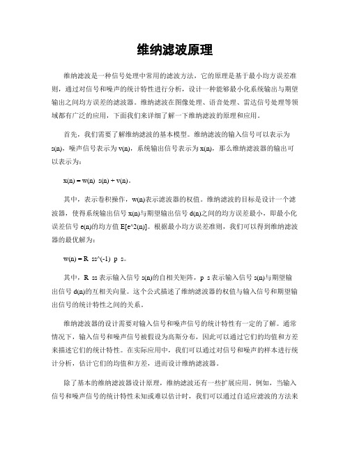
维纳滤波原理维纳滤波是一种信号处理中常用的滤波方法,它的原理是基于最小均方误差准则,通过对信号和噪声的统计特性进行分析,设计一种能够最小化系统输出与期望输出之间均方误差的滤波器。
维纳滤波在图像处理、语音处理、雷达信号处理等领域都有广泛的应用,下面我们来详细了解一下维纳滤波的原理和应用。
首先,我们需要了解维纳滤波的基本模型。
维纳滤波的输入信号可以表示为s(n),噪声信号表示为v(n),系统输出信号表示为x(n),那么维纳滤波器的输出可以表示为:x(n) = w(n) s(n) + v(n)。
其中,表示卷积操作,w(n)表示滤波器的权值。
维纳滤波的目标是设计一个滤波器,使得系统输出信号x(n)与期望输出信号d(n)之间的均方误差最小,即最小化误差信号e(n)的均方值E[e^2(n)]。
根据最小均方误差准则,我们可以得到维纳滤波器的最优解为:w(n) = R_ss^(-1) p_s。
其中,R_ss表示输入信号s(n)的自相关矩阵,p_s表示输入信号s(n)与期望输出信号d(n)的互相关向量。
这个公式描述了维纳滤波器的权值与输入信号和期望输出信号的统计特性之间的关系。
维纳滤波器的设计需要对输入信号和噪声信号的统计特性有一定的了解。
通常情况下,输入信号和噪声信号被假设为高斯分布,因此可以通过它们的均值和方差来描述它们的统计特性。
在实际应用中,我们可以通过对信号和噪声的样本进行统计分析,估计它们的均值和方差,进而设计维纳滤波器。
除了基本的维纳滤波器设计原理,维纳滤波还有一些扩展应用。
例如,当输入信号和噪声信号的统计特性未知或难以估计时,我们可以通过自适应滤波的方法来实现维纳滤波。
自适应滤波器可以根据系统的实时输入信号和输出信号来动态地调整滤波器的权值,以适应信号和噪声的变化特性,从而实现更好的滤波效果。
维纳滤波在图像处理中有着广泛的应用。
在数字图像处理中,图像通常会受到噪声的影响,例如加性高斯噪声、椒盐噪声等。
旋转机械振动信号的小波域维纳滤波去噪
旋转机械振动信号的小波域维纳滤波去噪杨尚君;张峰;石现峰【摘要】In order to remove the noise in rotating machinery vibration signal during the acquisition and transmission process,the algorithm of Wiener filtering in wavelet domain is proposed to meet the requirements of vibration signal filtering,based on Wiener filtering and wavelet threshold filtering, through the establishment of rotating machinery vibration signal acquisition ing the rotating machinery vibration signal which is actual measurement in the industrial field, the algorithm is simulated.The result shows:This algorithm can maintain the linear phase characteristics for rotating machinery vibration signal,the filtered signal doesn't produce the amplitude distortion;The mean square error of Wiener filtering in wavelet domain is less than that of Wiener filtering and wavelet threshold filtering.The denoising result is better than Wiener filtering and wavelet threshold filtering.%为了去除旋转机械振动信号采集传输过程中混入的噪声干扰,文中基于维纳滤波和小波阈值滤波,通过建立旋转机械振动信号采集模型,结合振动信号滤波要求,提出了旋转机械振动信号的小波域维纳滤波算法.利用工业现场旋转机械实测振动信号,对该算法进行仿真.结果表明:该算法保持了旋转机械振动信号的线性相位特性,滤波后信号未产生明显的幅度失真;小波域维纳滤波的均方误差小于维纳滤波和小波阈值滤波,去噪效果优于维纳滤波和小波阈值滤波.【期刊名称】《西安工业大学学报》【年(卷),期】2016(036)010【总页数】5页(P856-860)【关键词】旋转机械;振动;小波域维纳滤波;线性相位【作者】杨尚君;张峰;石现峰【作者单位】西安工业大学电子信息工程学院,西安 710021;西安工业大学电子信息工程学院,西安 710021;西安工业大学电子信息工程学院,西安 710021【正文语种】中文【中图分类】TN911.4旋转机械故障检测采用数字信号处理的方法对实际测量的振动信号进行分析,用以参数检测和质量评价.在采集及传输的过程中,振动信号不可避免的混入噪声干扰,对振动信号的滤波处理既要取得较好的效果,也要保证振动信号的均衡相位,以便根据这些特性,来进行状态检测和故障诊断,应用于旋转机械振动信号的滤波处理当中.传统的有限冲击响应(Finite Impulse Response,FIR)滤波器和无限冲击响应(Infinite Impulse Response,IIR)滤波器,两者的滤波算法滤波效果和线性相位之间难以达到均衡[1];文献[2]采用维纳滤波对非平稳振动信号进行处理,研究表明未达到预期效果;文献[3]采用循环维纳滤波对振动信号进行周期性的分段处理,每段采用维纳滤波方法,有效的去除了自适应噪声,但是循环维纳滤波算法复杂度大;文献[4]基于离散余弦变换(Discrete Cosine Transform,DCT)算法,保留了信号的部分离散余弦变换域的点数,实现了数据的压缩,但是DCT滤波算法对于大数据的压缩存在着数据丢失,滤波效果差的问题.针对振动信号滤波的敏感相位和滤波效果的问题,文中将维纳滤波和小波阈值滤波相结合,通过建立旋转机械振动信号采集模型,结合振动信号滤波要求,提出旋转机械振动信号的小波域维纳滤波算法.利用工业现场旋转机械实测振动信号,对该算法进行仿真,以期满足滤波要求和线性相位,以适用于其他一维含噪信号的处理.旋转机械振动信号的采集模型如图1所示.图1中ω为旋转机械转轴转动的角频率,v为转轴转动的线速度,理想情况下振动信号可表示为y=A+Bcos(ωt+φ)信号处理前将其直流分量去除,随机变量φ服从在[0,2π]区间的均匀分布,根据平稳随机过程的定义,有E(y)=E[Bcos(ωt+φ)]=Ry(t1,t2)=E[y(t1)y(t2)]=根据工业现场的实际情况,对旋转机械实际振动信号进行实际采集.数据采集的相关参数如下:32倍频采样,采样频率为1 600 Hz,每通道连续采集128点.较为理想情况下,振动信号的时域波形如图2所示.为研究去噪性能,对信号加入非平稳随机噪声,噪声点数为达到与采样点数匹配,故取128点,加噪后的振动信号如图3所示.理想状况下,振动信号各次谐波的谱峰位置应出现在50 Hz的整倍频处,谱峰位置包含了转轴运行状态的有用信息,因此谱峰的准确性直接影响了后期的故障诊断.而初始相位的偏移会导致振动信号后期谱估计中谱峰的分裂或偏移,因此对于振动信号的滤波,单位冲击响应应具有较高的线性相位[5].振动信号频谱图的方差和分辨力性能也直接受到噪声的影响,因此为了获得较好性能的方差和分辨力,应尽可能的对振动信号的噪声进行去除.经典的FIR滤波器和IIR滤波器在滤波效果和线性相位方面均难以满足要求,故需要引入现代的维纳滤波算法来进行处理.根据最小均方误差准则[6],提出一种针对平稳过程的最优估计器.假定观测信号模型为x(n)=s(n)+w(n)式中:s(n)为真实信号;w(n)为加性高斯白噪声,其分布为w(n)~N(0,δ2).根据FIR滤波器准则,有维纳滤波算法原理如图4所示.其中Z-1表示Z变换,e(n)表示真实信号与滤波后信号的误差.均方误差为若使均方误差最小,应满足维纳霍夫方程通过图5可以看出,振动信号的维纳滤波算法保持了信号的初始相位均衡,但滤波效果较差,达不到后期信号处理的要求.根据小波阈值滤波,对含噪声信号进行正交小波变换.选择合适的小波基函数和分解小波层数,对含噪信号进行正交小波分解,得到对应的小波分解系数,其中包含了低频系数和高频系数.选择合适的阈值,对分解后的系数进行阈值处理.每一层小波系数再进行量化处理.进行小波反变换.将阈值处理后的小波系数进行重构,得到小波阈值滤波后的信号.实验选用软阈值函数进行处理[8],数学表达式为δ(σ)=sgn(σ)(|σ|-λ),|ω|>λ根据选用的Coif5小波基,分解2层,小波阈值滤波的结果如图6所示.从图6中可以看出,直接进行小波阈值去噪处理的信号取得了较好的平滑特性,但滤波后信号产生了失真,不能作为后期的信号处理对象.利用Haar小波作为小波基将信号从时域转化为小波域[9].Haar小波基函数为对于非平稳过程,功率谱密度与频率的幂成反比的,振动信号在经小波变换后能够,不同尺度间较强的相关性可有效去除,可以认为非平稳信号在经过小波变换后起到了信号的白化作用[10],满足上述结果的条件须进行正交小波变换,Haar小波作为简单的正交函数,将振动信号从时域转化到小波域选用Haar小波,降低了信号的非平稳特性的同时,保留了信号的有用信息[11-12].根据维纳滤波的原理,在构建维纳霍夫方程前需已知加噪信号和期望信号,利用小波阈值去噪对加噪振动信号进行简单的阈值去噪处理,将原始振动信号作为期望信号,两者同时变换到小波域进行维纳滤波处理[13].小波域维纳滤波算法过程如下:① 将加噪的振动信号进行小波阈值去噪进行预处理,得到信号,用于构建小波域的维纳霍夫方程;② 分别将原始振动信号(作为期望信号)和小波阈值去噪信号两者分别利用Haar小波进行小波变换,分别提取两者的近似分量和细节分量;③ 利用两者细节分量构建维纳霍夫方程,对小波阈值去噪信号的细节分量进行滤波处理,利用两者近似分量构建维纳霍夫方程,对小波阈值去噪信号的近似分量进行滤波处理;④ 利用小波反变换函数对上述信号处理结果进行反变换,其利用的小波基仍为Haar小波.小波域32阶次维纳滤波算法信号处理结果如图7所示.通过图7和图5的对比,小波域维纳滤波算法具有较好的线性相位特性,振动信号初始相位没有发生明显偏移.在小波域维纳滤波的滤波阶数小于维纳滤波阶数的同时,小波域维纳滤波能取得更好的滤波效果.根据图7和图6的比较,利用小波阈值滤波算法保证了振动信号滤波后的平滑特性,该算法可用于实际的振动信号去噪环境中.由于计算量较大,该算法可做振动信号的离线分析处理.分别计算各种算法滤波后的结果与原始振动信号做均方误差的求解,进行算法性能定量分析和对比,得出数据见表1.从表1可看出,小波域维纳滤波的均方误差要小于维纳滤波和小波阈值滤波,小波域维纳滤波算法性能优于各种单独算法,小波域维纳滤波算法滤波后的信号更接近原始的振动信号.利用小波域维纳滤波算法对振动信号进行去噪处理,对其结果进行频谱分析,采取周期图法,功率谱密度(Power Spectral Density,PSD)估计图如图8所示.f为频率,DPS为功率谱密度.根据振动信号的采集模型,信号每周期采样32点,采样频率为1 600 Hz,因此信号的固有频率为50 Hz.从图8中可以看出,滤波后振动信号的谱峰处于50 Hz 整倍频处,功率谱图中的谱峰具有较好的尖锐程度,分辨率性能较好,具有较强辨别信号的能力,且谱峰没有发生偏移或分裂的现象.因此滤波后的振动信号适用于后期的旋转机械故障检测.1) 将振动信号从时域转化到小波域,降低了振动信号的非平稳特性,小波域维纳滤波算法保留了维纳滤波算法的线性相位特性,信号原有的初始相位未发生偏移,滤波后的信号幅值和相位未产生失真.2) 小波域维纳滤波去噪性能优于维纳滤波和小波阈值滤波,均方误差小于维纳滤波和小波阈值滤波.3) 小波域维纳滤波后的振动信号,功率谱图中的谱峰处于50 Hz整倍频处,分辨率性能好,辨别信号的能力优于维纳滤波,谱峰没有发生偏移或分裂,适用于后期的旋转机械故障检测.ZHANG Feng,SHI Xianfeng,ZHANG Xuezhi.Principle and Application of Digital Signal Processing[M].Beijing:Electronics Industry Press,2012.(in Chinese)MING Yang.Study on Cyclostationarity and Blind Source Separation-Based Rolling Element Bearing Fault Feature Extraction[D].Shanghai:Shanghai Jiao Tong University,2013.(in Chinese)MING Yang,CHEN Jin,DONG Guangming.Rolling Bearing Fault Diagnosis Based on Cyclic Wiener Filtering and Envelop Spectrum[J].Journal of Vibration Engineering,2010,23(5):537.(in Chinese)GUAN Bo,HU Jinsong.Research on the Method of the Vibration Signal of Rotating Machinery Based on DCT[J].Turbine Technology,2007,49(4):285. (in Chinese)LI Nan.Study on the Speech Antinoise Based on Wavelet Transform and Wiener Filtering[J].Electro Acoustic Technology,2007,31(5):46.(in Chinese) YANG Lingxiang,YAO Bin.Denoisng Method via Local Wiener Filtering in Wavelet Domain Based on Canny Operator[J].Journal of Bingtuan Education Institute,2009,19(5):35.(in Chinese)LI Dongbing,LI Guoping,TENG Guowei,et al.New Method of De-noising Based on Wavelet and Wiener Filtering[J].VideoEngineering,2013,37(13):26.(in Chinese)HU Yaobin,CHEN Aihua,ZHANG Chunliang.Research of Denoising Technology about Wavelet Analysis with Wiener Filter[J].Communication of Power System,2006,27(162):42.(in Chinese)。
Chapter 5-维纳滤波

23/31
5.4 维纳滤波器的应用……
应用例子1:维纳滤波方法提取脑电诱发电位 维纳滤波器的传递函数:
S s ( w, i ) Ss ( w) 相干函数加权构造的维纳滤波器:H ( w, i ) H ( w) S ( w, i ) S ( w) S s ( w, i ) n S s ( w) n N N
2016/6/10
30/31
下集预告
第六章 卡尔曼滤波
2016/6/10
31/31
实验三详解……
源程序:
clear all np = 0:99; % p = sin(pi/5*np); % 正弦 % p = exp(-0.06*np); % 指数衰减 % p = sin(pi/5*np).*exp(-0.06*np); % 指数衰减正弦 p = ones(size(np)); % 方波 figure; p = [p,zeros(1,length(x)-length(p))]; % 如果要求归一化相关系数 subplot(2,2,1); plot(np,p); (相干系数),两个序列要同样长 Rpw = xcorr(w,p,'coeff'); n = 0:1000; Rps = xcorr(s,p,'coeff'); w = randn(size(n)); Rpx = xcorr(x,p,'coeff'); s = zeros(size(n)); n2 = (n(1)-n(end)):(n(end)-n(1)); A = 3; % 衰减系数 figure; s(100:199) = s(100:199)+A*p; subplot(3,1,1); plot(n2,Rpw); title('Rpw of p(n) and s(500:599) = s(500:599)+A/3*p; w(n)');title('Rpw of p(n) and w(n)'); s(800:899) = s(800:899)+A/3/3*p; subplot(3,1,2); plot(n2,Rps); title('Rps of p(n) and s(n)');title('Rps x = s+w; of p(n) and s(n)'); figure; subplot(3,1,3); plot(n2,Rpx); title('Rpx of p(n) and subplot(3,1,1); plot(n,w); title('Noise'); x(n)');title('Rpx of p(n) and x(n)'); subplot(3,1,2); plot(n,s); title('Signal'); subplot(3,1,3); plot(n,x); title('Signal with Noise'); 2016/6/10 32/31
第八章 维纳滤波
rxx(λ-k)
rzx(λ)
第八章 维纳滤波 维纳-何甫积分方 程式(离散形式):
中原工学院
N xx
机电学院
h(k )r
k 0
N
( k ) rzx ( ) 或 h(k )rxx (k ) rzx ( )
k 0
自相关函数为偶函数
▲ 维纳滤波器 如果已知x(n)与所要求的输出信号z(n),则当x(n)的自相关函 数和z(n)与x(n)的互相关函数为已知时,求解维纳-何甫方程,即可求得满足均 方误差最小的滤波因子h(n)。这就是按照最小平方准则设计的线性滤波系统, 它是一个最佳系统,通常称为维纳滤波器。 这是一个对 称 矩阵 。 卷积形式:
第八章 维纳滤波
中原工学院
机电学院
第二节
反滤波
一、回声鸣震现象及反滤波
问题的提出:在某些情况下(例如,在大礼堂内演讲,由于墙壁多次反射, 而造成回声交混,形成一片轰鸣声,使人们听不清讲话内容)所录取的信号, 可认为是原始信号经过几个物理系统(信号传输的路径或通道)作用的结果, 或者看成是源信号经过几个物理滤波器以串联形式滤波的结果。这时,采用 反滤波方法可以使真正源信号从干扰中恢复出来。
n n n n
期望输出s(n)与输入x(n)的互相关函数为
n n
rsx (k ) s(n k ) x(n) s(n k )[s(n) n(n)] rss (k )
如果以 Rss(ejω) 和 Rnn(ejω) 分别表示 rss(k) 和 rnn(k) 的频谱,即分别为 s(n) 和 n(n) 的功率谱,则在对维纳滤波的时间范围不加限制的情况下,由式H(ejω)=Rzs(ejω)/ Rxx(ejω),可以得到维纳滤波器的频率响应应为:
维纳滤波基本概念
Wiener 滤波概述Wiener 滤波器是从统计意义上的最优滤波,它要求输入信号是宽平稳随机序列,本章主要集中在FIR 结构的Wiener 滤波器的讨论。
由信号当前值与它的各阶延迟({n x )n ,§3.1从估计理论观点导出Wiener 滤波FIR 结构(也称为横向)的Wiener 滤波器的核心结构如图4所示. 图4.横向Wiener 滤波器FIR 结构的Wiener 是一个线性Beyesian 估计问题.为了与第2讲中估计理论一致,假设信号,滤波器权值均为实数由输入)(n x 和它的1至(M-1)阶延迟,估计期望信号)(n d ,确定权系数}1,0,{-=M i w i 使估计误差均方值最小,均方误差定义为:xx R 这里线性0w或a1) 波可能会达到更好结果。
2) 在联合高斯条件下,Wiener 滤波也是总体最优的(①从Bayesian 估计意义上讲是这样,②要满足平稳条件) 3) 从线性贝叶斯估计推导过程知,在滤波器系数取非最优的w 时,其误差性能表示:它是w 的二次曲面,只有一个最小点,0w w =时,m in )(J w J =§3.2维纳滤波:从正交原理和线性滤波观点分析Wiener 滤波器 Wiener 滤波器是一个最优线性滤波器,滤波器核是IIR 或FIR 的。
导出最优滤波器的正交原理,并从正交原理出发重新导出一般IIR 。
=∑∞=--0*)(][k kk n x w n d均方误差是:{}][*][n e n e E J ={}2|][|n e E = 设权系数:k k k jb a w +=定义递度算子Tk ],,[10 ∇∇∇=∇.其中k k k k b ja w ∂∂+∂∂=∂∂=∇符号J ∇是递度算子作用于J ,其中第k 项为:k k k b Jja J J ∂∂+∂∂=∇要求由J 得∇[nje J k由[e a k∂k 代入J k ∇表达式整理得:]][*][[2n e k n x E J k --=∇当0=∇Jk ,1,0=k 时,J 达到最小。
图像去模糊算法分析与研究
本科毕业设计(论文)题目: 图像去模糊算法对比分析研究学院:专业:班级:学号:学生姓名:指导教师:职称:二○一五年六月一日图像去模糊算法分析与研究摘要在数字时代,图像去模糊作为图像复原技术的一个分支,一直是一个具有挑战和吸引力的问题,具有重大的研究价值与社会意义。
图像去模糊技术近年来得到了广泛研究,在理论和算法上也愈加系统和成熟,根据图像模糊核是否已知,图像去模糊技术被分为非盲图像去模糊和盲图像去模糊两大类。
文章主要是选取几种典型的去模糊算法,在已知模糊核的基础上进行分析研究各算法的特点与去模糊效果的优劣性,即非盲去模糊算法的分析研究。
基于运动模糊和离焦模糊这两大模糊类型,对其分别在有噪声(本文指高斯白噪声)和无噪声情况下的实验结果进行分析比较。
文章首先介绍了两种主要模糊图像类型及其造成图像模糊的成因,并对各模糊类型的点扩散函数估计获取。
其次,是对图像基本退化模型的引入,从本质上了解图像模糊与去模糊的实质。
接着,我们介绍了两类典型的去模糊评价方法:峰值信噪比(Peak Signal to Noise Ratio)和平均结构相似性指数(Mean Structural Similarity Index)。
在这之后主要是算法比较,分类对几种典型的去模糊算法进行数学分析与讨论,包括用于去除运动模糊的Richardson-Lucy算法(即RL算法)和约束最小二乘法;用于去除离焦模糊的逆滤波算法和维纳滤波算法(Wiener filtering)。
最后对几种算法进行Matlab仿真实验设计,并对其结果与恢复效果分析总结。
关键词:离焦模糊;运动模糊;点扩散函数;算法比较;仿真设计AbstractIn digital times,image de—blurring as a branch of image restoration technology has been a hard and attractive problem. However, image restoration has great value of the research and social significance。
维纳滤波概述
E[ x(t ) h(t ) y (t )d ]2
0
E[ x(t )]2 2 h( )( E[ y (t ) y ( )]d
0
h( )d h( ) E[ y (t ) y (t )]d
0 0
Rxx (0) 2 h( ) Ryx ( )d
E[e 2 (n)] lim
(2-25)
1 T 2T
T
T
(n) s (n)]2 dn [s
滤波器在n时刻复现信号s(n)显然是滤波问题。这是一种简单的过滤,滤除 噪声v(n)是唯一的目的。 但输出在时间上的简单的超前或者滞后,都不失为线性
(n a) ,这显然是一种超前的情况,输 滤波问题。在n时刻,滤波器输出如果为 s (n a) 是 s(n a) 的估计值,它比x(n)超前了 时间。这个时候滤波器所完成 出s
2 J1 2 J 2 0( 3 )
(2-15) 则将导致
J[ h h( t )] J [ o p t( t ) oh p t (t ) ]
(2-16) 这明显与最佳冲击响应将使均方误差最小的假设相矛盾。所以,我们只能取
J1 =0,即满足式(2-11)。由式(2-13)知,若使 J1 =0成立,则必须使式(2-13)中的方
第 2 章 维纳滤波理论
2.1 维纳滤波的概述
维纳 (Wiener) 滤波是用来解决从噪声中提取信号问题的一种过滤 (或滤波) 的方法。 实际上这种线性的滤波问题,可以看成是一种估计问题或是一种线性估 计问题。 维纳滤波器是一种基于最小均方误差准则下的估计滤波器。 滤波器的输入包 括有真实信号值x(t)和干扰噪声w(t),信号值与噪声是统计独立的,则两者的合 成输入信号是