Notation The matrix
结果输出类关键abaqus

Strain outputThe total strain E is composed of the elastic(线性) strain EE, the inelastic (非线性)strain IE, and the thermal strain(热应变) THE. The inelastic strain IE consists of the plastic strain(塑性应变) PE and the creep strain (蠕变)CE.For geometrically nonlinear analysis (几何非线性分析)Abaqus/Standard makes it possible to output different strain measures as well as elastic and various inelastic strains. The various total strain measures (integrated strain measure(总应变量度) E, nominal strain measure(名义应变) NE, and logarithmic strain measure(对数应变量度) LE) are described in “Conventions,” Section 1.2.2. The default strain measure for output to the data (.dat) and results (.fil) files is E. However, for geometrically nonlinear analysis using element formulations (公式化)that support finite strains, E is not available for output to the output database (.odb) file, and LE is the default strain measure.Principal value outputOutput of the principal(主要的) values can be requested for stresses, strains, and other material tensors(张量). Either all principal values or the minimum, maximum, or intermediate (中间的)values canbe obtained. All principal values of tensor ABC are obtained with the request ABC P. The minimum, intermediate, and maximum principal values are obtained with the requests ABC P1, ABC P2, and ABC P3.For three-dimensional, (generalized) plane strain, and axisymmetric elements all three principal values are obtained. For plane stress, membrane(薄膜), and shell elements, the out-of-plane(平面外) principal value cannot be requested for history-type output. For field-type output, Abaqus/CAE always reports the out-of-plane principal value as zero. Principal values cannot be obtained for truss(桁架) elements or for any beam elements other than the three-dimensional beam elements with torsional(扭力的,扭转的)shear stresses.If a principal value or an invariant(不变量)is requested for field-type output, the output request is replaced with an output request for the components of the corresponding tensor. Abaqus/CAE calculates all principal values and invariants from these components. If a principal value is desired as history-type output, it must be explicitly(明白的,明确的)requested since Abaqus/CAE does no calculations on history data.Tensor outputTensor variables that are written to the output database as field-type output are written as components in either the default directions defined by the convention(按照惯例) given in “Orientations,”Section 2.2.5 (global directions for solid elements, surface directions for shell and membrane(薄膜) elements, and axial and transverse (横切的,横断的)directions for beam elements), or the user-defined local system. Abaqus/CAE calculates all principal values and invariants(不变量) from these components. See “Writing field output data,” Section 9.6.4 of the Abaqus Scripting User's Manual, for a description of the different types of tensor variables.For plane stress, membrane, and shell elements, only the in-plane(平面内) tensor components (11, 22, and 12 components) are stored by Abaqus/Standard. The out-of-plane(平面外) direct component for stress (S33) is reported as zero to the output database as expected, and the out-of-plane component of strain (E33) is reported as zero even though it is not(此时E33值是失真的). This is because the thickness direction is computed based on section properties rather than at the material level. The out-of-plane components can be requested for field-type output and cannot be requested for history-type output. The out-of-plane stress components are not reported to the data (.dat) file or to the results (.fil) file.For three-dimensional beam elements with torsional(扭力的,扭转的) shear stresses, only the axial and the torsional components (the 11 and 12 components) are stored by Abaqus/Standard. The other direct component (the 22 component) is reported as zero for field-type outputand cannot be requested for history-type output.The components for tensor variables are written to the output database in single precision(单精度). Therefore, a small amount of precision roundoff error(舍入误差) may occur when calculating the variables' principal values. Such roundoff error may be observed(观察、研究), for example, when analytically zero values are calculated as relatively small nonzero values.Element integration point variablesYou can request element integration point variable output to the data, results, or output database file (see “Element output” in “Output to the data and results files,” Section 4.1.2, and “Element output” in “Output to the output database,” Section 4.1.3).Tensors and associated principal values and invariantsSAll stress components..dat: yes .fil: yes .odb Field: yes .odb History: yesSij-component of stress ()..dat: yes .fil: no .odb Field: no .odb History: yesSPAll principal stresses (三个主应力)..dat: yes .fil: yes .odb Field: yes .odb History: yesSP nMinimum, intermediate (中间的), and maximum principal stresses (SP1 SP2 SP3).(123σσσ≥≥).dat: yes .fil: no .odb Field: no .odb History: yesSINVAll stress invariant components (MISES, TRESC, PRESS, INV3). For field output SINV is converted to a request for the generic variable S. .dat: yes .fil: yes .odb Field: yes .odb History: yesINV3(I 3):x 3x y x z x yy y z x z y z z I στττστττσ⎛⎫ ⎪= ⎪ ⎪⎝⎭MISES Mises equivalent stress, defined as28222,k ()3J J τ==畸变能条件参考《弹塑性力学引论》,杨桂通P60.where is the deviatoric stress tensor (偏应力张量 ), defined aswhere is the stress, p is the equivalent pressure stress (各向相等的压或拉应力) (defined below), and is a unit matrix (单位矩阵). In index notationwhere , , and is the Kronecker delta(柯氏σ). 1i 0ij j i j σ--=⎧=⎨--≠⎩当当,x i x x m y x z j y y m y z x z y z z m S σστττσστττσσ⎡⎤-⎢⎥=-⎢⎥⎢⎥-⎣⎦.dat: yes .fil: no .odb Field: no .odb History: yesMISESMAXMaximum Mises stress among all of the section points. For a shell element it represents the maximum Mises value among all the section points in the layer, for a beam element it is the maximum Mises stress among all the section points in the cross-section 横截面图, and for a solid element it represents the Mises stress at the integration points. .dat: no .fil: no .odb Field: yes .odb History: noTRESCTresca equivalent stress, defined as the maximum difference between principal stresses (主应力)..dat: yes .fil: no .odb Field: no .odb History: yesPRESSEquivalent pressure stress, defined as.dat: yes .fil: no .odb Field: no .odb History: yesINV3Third stress invariant (第三应力不变量), defined aswhere is the deviatoric stress(偏应力)defined in the context of Mises equivalent stress, above..dat: yes .fil: no .odb Field: no .odb History: yesTRIAXStress triaxiality三轴应力, ..dat: no .fil: no .odb Field: yes .odb History: yesALPHAAll total kinematic(运动学上的)hardening shift tensor components..dat: yes .fil: yes .odb Field: yes .odb History: yesALPHA ij-component of the total shift tensor ()..dat: yes .fil: no .odb Field: no .odb History: yesALPHA kAll kinematic hardening shift tensor components (). .dat: no .fil: no .odb Field: yes .odb History: yesALPHA k_ij-component of the kinematic hardening shift tensor (and )..dat: no .fil: no .odb Field: no .odb History: yesALPHANAll tensor components of all the kinematic hardening shift tensors,except the total shift tensor, ALPHA..dat: no .fil: no .odb Field: yes .odb History: yesALPHAPAll principal values of the total shift tensor(总位移张量)..dat: yes .fil: yes .odb Field: yes .odb History: yesALPHAP nMinimum, intermediate, and maximum principal values of the total shift tensor (ALPHAP1 ALPHAP2 ALPHAP3)..dat: yes .fil: no .odb Field: no .odb History: yesEAll strain components. For geometrically nonlinear analysis using element formulations that support finite strains(有限应变), E is not available for output to the output database (.odb) file..dat: yes .fil: yes .odb Field: yes .odb History: yesEij-component of strain ()..dat: yes .fil: no .odb Field: no .odb History: yesEPAll principal strains..dat: yes .fil: yes .odb Field: yes .odb History: yesEP nMinimum, intermediate, and maximum principal strains (EP1 EP2 EP3)..dat: yes .fil: no .odb Field: no .odb History: yesNEAll nominal strain(名义应变)components..dat: yes .fil: yes .odb Field: yes .odb History: yesNE ij-component of nominal strain ()..dat: yes .fil: no .odb Field: no .odb History: yesNEPAll principal nominal strains..dat: yes .fil: yes .odb Field: yes .odb History: yesNEP nMinimum, intermediate, and maximum principal nominal strains (NEP1 NEP2 NEP3)..dat: yes .fil: no .odb Field: no .odb History: yesLEAll logarithmic strain components. For geometrically nonlinear analysis using element formulations that support finite strains, LE is the default strain measure for output to the output database (.odb) file..dat: yes .fil: yes .odb Field: yes .odb History: yesLE ij-component of logarithmic strain ()..dat: yes .fil: no .odb Field: no .odb History: yesLEPAll principal logarithmic strains..dat: yes .fil: yes .odb Field: yes .odb History: yesLEP nMinimum, intermediate, and maximum principal logarithmic(对数的)strains (LEP1 LEP2 LEP3)..dat: yes .fil: no .odb Field: no .odb History: yesERAll mechanical strain rate(机械应变率)components..dat: yes .fil: yes .odb Field: yes .odb History: yesER ij-component of strain rate ()..dat: yes .fil: no .odb Field: no .odb History: yesERPAll principal mechanical strain rates..dat: yes .fil: yes .odb Field: yes .odb History: yesERP nMinimum, intermediate, and maximum principal mechanical strain rates (ERP1 ERP2 ERP3)..dat: yes .fil: no .odb Field: no .odb History: yesDGAll components of the total deformation gradient(总变形梯度). Available only for hyperelasticity(超弹性), hyperfoam(泡沫橡胶), and material models defined in user subroutine UMAT. For fully integrated first-order quadrilaterals(一阶四边形)and hexahedra(六面体), the selectively reduced integration(缩减积分)technique is used. A modified(修正的)deformation gradient is output for these elements. .dat: yes .fil: yes .odb Field: no .odb History: noDG ij-component of the total deformation gradient ()..dat: yes .fil: no .odb Field: no .odb History: noDGPPrincipal stretches主伸长量..dat: yes .fil: yes .odb Field: no .odb History: noDGP nMinimum, intermediate, and maximum values of principal stretches(DGP1 DGP2 DGP3)..dat: yes .fil: no .odb Field: no .odb History: noEEAll elastic strain(弹性应变)components..dat: yes .fil: yes .odb Field: yes .odb History: yesEE ij-component of elastic strain ()..dat: yes .fil: no .odb Field: no .odb History: yesEEPAll principal elastic strains..dat: yes .fil: yes .odb Field: yes .odb History: yesEEP nMinimum, intermediate, and maximum principal elastic strains (EEP1 EEP2 EEP3)..dat: yes .fil: no .odb Field: no .odb History: yesIEAll inelastic strain(非弹性应变)components..dat: yes .fil: yes .odb Field: yes .odb History: yesIE ij-component of inelastic strain ()..dat: yes .fil: no .odb Field: no .odb History: yesIEPAll principal inelastic strains..dat: yes .fil: yes .odb Field: yes .odb History: yesIEP nMinimum, intermediate, and maximum principal inelastic strains (IEP1 IEP2 IEP3)..dat: yes .fil: no .odb Field: no .odb History: yesPEAll plastic strain components. This identifier also provides PEEQ, ayes/no flag telling if the material is currently yielding(屈服)or not (AC YIELD: “actively yielding”; that is, the plastic strain changed during the increment), and PEMAG when PE is requested for the data or results files. When PE is requested for field output to the output database, PEEQ(等效塑性应变)is also provided..dat: yes .fil: yes .odb Field: yes .odb History: yesPE ij-component of plastic strain ()..dat: yes .fil: no .odb Field: no .odb History: yesPEEQEquivalent plastic strain. This identifier also provides a yes/no flag (1/0 on the output database) telling if the material is currently yielding or not (AC YIELD: “actively yielding”; that is, the plastic strain changed during the increment).The equivalent plastic strain is defined as , where is the initial equivalent plastic strain.The definition of depends on the material model. For classical metal (Mises) plasticity . For other plasticity models,see the appropriate section in Part V, “Materials.”When plasticity occurs in the thickness direction(厚度方向)to a gasket垫圈element whose plastic behavior is specified as part of a gasket behavior definition, PEEQ is PE11..dat: yes .fil: no .odb Field: yes .odb History: yesPEEQMAXMaximum equivalent plastic strain, PEEQ, among all of the section points. For a shell element it represents the maximumPEEQ value among all the section points in the layer, for a beam element it is the maximum PEEQ among all the section points in the cross-section(横断面), and for a solid element it represents thePEEQ at the integration points(积分点). .dat: no .fil: no .odb Field: yes .odb History: noPEEQTEquivalent plastic strain in uniaxial tension单轴向张力for cast iron (铸铁,生铁), Mohr-Coulomb tension cutoff(抗拉伸强度), and concrete damaged plasticity, which is defined as . This identifier also provides a yes/no flag (1/0 on the output database) telling if the material is currently yielding or not (AC YIELDT: “actively yielding”; that is,the plastic strain changed during the increment)..dat: yes .fil: yes .odb Field: yes .odb History: yesPEMAGPlastic strain magnitude, defined as .For most materials, PEEQ and PEMAG are equal only for proportional loading比例加荷. When plasticity occurs in the thickness direction to a gasket(垫圈)element whose plastic behavior is specified as part of a gasket behavior definition, PEMAG is PE11..dat: yes .fil: no .odb Field: yes .odb History: yesPEPAll principal plastic strains(主应变)..dat: yes .fil: yes .odb Field: yes .odb History: yesPEP nMinimum, intermediate, and maximum principal plastic strains (PEP1 PEP2 PEP3)..dat: yes .fil: no .odb Field: no .odb History: yesCEAll creep strain(蠕变应变)components. This identifier also provides CEEQ, CESW, and CEMAG when CE is requested for the data or results files.CE ij-component of creep strain ()..dat: yes .fil: no .odb Field: no .odb History: yesCEEQEquivalent creep strain, defined as .The definition of depends on the material model. For classical metal (Mises) creep . For other creep models, see the appropriate section in Part V, “Materials.”When creep occurs in the thickness direction to a gasket element whose creep behavior is specified as part of a gasket behavior definition, CEEQ is CE11..dat: yes .fil: no .odb Field: yes .odb History: yesCESWMagnitude of swelling strain(膨胀应变).For cap creep CESW gives the equivalent creep strain produced by the consolidation creep mechanism(蠕变机理), defined as , where is the equivalent creep pressure,CEMAGMagnitude of creep strain (defined by the same formula given above for PEMAG, applied to the creep strains)..dat: yes .fil: no .odb Field: yes .odb History: yesCEPAll principal creep strains..dat: yes .fil: yes .odb Field: yes .odb History: yesCEP nMinimum, intermediate, and maximum principal creep strains (CEP1 CEP2 CEP3)..dat: yes .fil: no .odb Field: no .odb History: yesAdditional element stressesCS11Average contact pressure(平均接触压力)for link and three-dimensional line gasket elements. Available only if the gasket contact area is specified; see “Defining the contact area for average contact pressure output” in “Defining the gasket behavior directly usi ng a gasket behavior model,” Section 29.6.6..dat: yes .fil: yes .odb Field: yes .odb History: yesTSHRAll transverse shear stress(横向剪切应力)components. Available only for thick shell elements such as S3R, S4R, S8R, and S8RT. Contouring of this variable is supported in the Visualization module of Abaqus/CAE. .dat: yes .fil: yes .odb Field: yes .odb History: yesTSHR i3-component of transverse shear stress (). Available only for thick shell elements(壳单元)such as S3R, S4R, S8R, and S8RT..dat: yes .fil: no .odb Field: no .odb History: yesCTSHRTransverse shear stress(横向剪切应力)components for stacked continuum shell elements. Available only for SC6R and SC8R elements. Contouring of this variable is supported in the Visualization module of Abaqus/CAE..dat: yes .fil: no .odb Field: yes .odb History: yesCTSHR i3-component of transverse shear stress (). Available only for SC6R and SC8R elements..dat: yes .fil: no .odb Field: no .odb History: yesSSAll substresses. Available only for ITS elements..dat: yes .fil: yes .odb Field: no .odb History: noSS nn th substress (). Available only for ITS elements..dat: yes .fil: no .odb Field: no .odb History: noVibration and acoustic quantitiesINTENVibration intensity(震动强度). Available only for the steady-state dynamics procedure. For real-only steady-state dynamics analyses, the intensity is a pure imaginary(纯虚数)vector, but it is stored as real on the output database. Available for structural, solid, and acoustic(声学的)elements and for rebar(钢筋)..dat: no .fil: no .odb Field: yes .odb History: yesACVAcoustic particle velocity声学的质点速度. Available only if the steady-state dynamic procedure is used, and available only for acoustic finite elements..dat: no .fil: no .odb Field: yes .odb History: yesACV nComponent n of the acoustic particle velocity vector (n= 1, 2, 3). Available only if the steady-state dynamic procedure is used, and available only for acoustic finite elements..dat: no .fil: no .odb Field: no .odb History: yesGRADPAcoustic pressure gradient(声压梯度). Available only if the steady-state dynamic procedure is used, and available only for acoustic finite elements..dat: no .fil: no .odb Field: yes .odb History: yesEnergy densities(密度)ENERAll energy densities. None of the energy densities are available in mode-based procedures; a limited number of them are available for direct-solution steady-state dynamic and subspace-based steady-state dynamic analyses. In steady-state dynamics all energy quantities are net per-cycle values, unless otherwise noted (see “Energy balance,” Section 1.5.5 of the Abaqus Theory Manual)..dat: yes .fil: yes .odb Field: yes .odb History: yesSENERElastic strain energy density (with respect to current volume). When the Mullins effect马林斯效应is modeled with hyperelastic materials超弹性材料, this quantity represents only the recoverable(可重获的)part of energy per unit volume(每单位体积). This is the only energy density available in the data file for eigenvalue extraction procedures(特征值提取过程); to obtain this quantity for eigenvalue extraction procedures in the results file or as field output in the output database, request ENER. In steady-state dynamic analysis this is the cyclic mean value(周期平均值)..dat: yes .fil: no .odb Field: yes .odb History: yesPENEREnergy dissipated(能量消耗)by rate-independent(率不相关)and rate-dependent plasticity, per unit volume. Not available for steady-state dynamic analysis..dat: yes .fil: no .odb Field: yes .odb History: yesCENEREnergy dissipated by creep, swelling, and viscoelasticity, per unit volume. Not available for steady-state dynamic analysis..dat: yes .fil: no .odb Field: yes .odb History: yesVENEREnergy dissipated by viscous effects(粘滞效应)(except those from viscoelasticity粘弹性and static静电dissipation), per unit volume..dat: yes .fil: no .odb Field: yes .odb History: yesEENERElectrostatic energy density. Not available for steady-state dynamic analysis..dat: yes .fil: no .odb Field: yes .odb History: yesJENERElectrical energy dissipated as a result of the flow of current电流、水流, per unit volume. Not available for steady-state dynamic analysis. .dat: yes .fil: no .odb Field: yes .odb History: yesDMENEREnergy dissipated by damage, per unit volume. Not available for steady-state dynamic analysis..dat: yes .fil: no .odb Field: yes .odb History: yesState, field, and user-defined output variablesSDVSolution-dependent state variables..dat: yes .fil: yes .odb Field: yes .odb History: yesSDV nSolution-dependent state variable n..dat: yes .fil: no .odb Field: yes .odb History: yesTEMPTemperature..dat: yes .fil: yes .odb Field: yes .odb History: yesFVPredefined field variables(预定义场变量). .dat: yes .fil: yes .odb Field: yes .odb History: yesFV nPredefined field variable n..dat: yes .fil: no .odb Field: yes .odb History: yesMFRPredefined mass flow rates..dat: yes .fil: yes .odb Field: yes .odb History: yesMFR nComponent n of predefined mass flow rate ()..dat: yes .fil: no .odb Field: no .odb History: yesUVARMUser-defined output variables(自定义输出变量). .dat: yes .fil: yes .odb Field: yes .odb History: yesUVARM nUser-defined output variable n..dat: yes .fil: no .odb Field: yes .odb History: yesComposite failure measuresCFAILUREAll failure measure components..dat: yes .fil: yes .odb Field: yes .odb History: yesMSTRSMaximum stress theory(最大应力理论)failure measure. .dat: yes .fil: no .odb Field: yes .odb History: yesTSAIHTsai-Hill theory failure measure..dat: yes .fil: no .odb Field: yes .odb History: yesTSAIWTsai-Wu theory failure measure..dat: yes .fil: no .odb Field: yes .odb History: yesAZZITAzzi-Tsai-Hill theory failure measure..dat: yes .fil: no .odb Field: yes .odb History: yesMSTRNMaximum strain theory(最大变形理论)failure measure. .dat: yes .fil: no .odb Field: yes .odb History: yesFluid link(流体连接器)quantitiesMFLCurrent value of the mass flow rate..dat: yes .fil: yes .odb Field: yes .odb History: yesMFLTCurrent value of the total mass flow..dat: yes .fil: yes .odb Field: yes .odb History: yesFracture mechanics(断裂理论学)quantitiesJKJ-integral, stress intensity factors. Available only for line spring elements. Output is in the following order for LS3S elements: J, K, , and . Output is in the following order for LS6 elements: J, , , , , and ..dat: yes .fil: yes .odb Field: yes .odb History: yesConcrete cracking and additional plasticityCRACKUnit normal to cracks in concrete..dat: yes .fil: yes .odb Field: no .odb History: noCONFNumber of cracks at a concrete material point..dat: yes .fil: yes .odb Field: no .odb History: noPEQCAll equivalent plastic strains when the model has more than one yield/failure surface..dat: yes .fil: yes .odb Field: yes .odb History: yesPEQC nn th equivalent plastic strain ().For jointed materials: PEQC provides equivalent plastic strains for all four possible systems (three joints - PEQC1, PEQC2, PEQC3, and bulk material - PEQC4). This identifier also provides a yes/no flag (1/0 on the output database) telling if each individual system is currently yiel ding or not (AC YIELD: “actively yielding”; that is, the plastic strain changed during the increment).For cap plasticity: PEQC provides equivalent plastic strains for all three possible yield/failure surfaces (Drucker-Prager failure surface - PEQC1, cap surface - PEQC2, and transition surface - PEQC3) and the total volumetric inelastic strain (PEQC4). All identifiers also provide a yes/no flag (1/0 on the output database) telling whether the yield surfaceis currently active or not (AC YIELD: “actively yielding”, that is, the plastic strain changed during the increment).When PEQC is requested as output to the output database, the active yield flags for each component are named AC YIELD1, AC YIELD2, etc. and take the value 1 or 0..dat: yes .fil: no .odb Field: no .odb History: yesConcrete damaged plasticityDAMAGECCompressive damage variable, ..dat: yes .fil: no .odb Field: yes .odb History: yesDAMAGETTensile damage variable, ..dat: yes .fil: no .odb Field: yes .odb History: yesSDEGScalar stiffness degradation variable, d..dat: yes .fil: no .odb Field: yes .odb History: yesPEEQEquivalent plastic strain in uniaxial compression, which is defined as . This identifieralso provides a yes/no flag (1/0 on the output database) telling if the material is currently undergoing compressive failure or not (AC YIELD: “actively yielding”; that is, the plastic strain changed during the increment)..dat: yes .fil: yes .odb Field: yes .odb History: yesRebar quantitiesRBFORForce in rebar..dat: yes .fil: yes .odb Field: yes .odb History: yesRBANGAngle in degrees between rebar and the user-specified isoparametric direction. Available only forshell, membrane, and surface elements..dat: yes .fil: yes .odb Field: yes .odb History: yesRBROTChange in angle in degrees between rebar and the user-specified isoparametric direction. Available only for shell, membrane, and surface elements..dat: yes .fil: yes .odb Field: yes .odb History: yesHeat transfer(热传递)analysisHFLCurrent magnitude and components of the heat flux per unit area vector. The integration points for these values are located at the Gauss points..dat: yes .fil: yes .odb Field: yes .odb History: yesHFLMCurrent magnitude of heat flux per unit area vector..dat: yes .fil: no .odb Field: no .odb History: yesHFL nComponent n of the heat flux vector ()..dat: yes .fil: no .odb Field: no .odb History: yesMass diffusion(质量扩散)analysisCONCMass concentration..dat: yes .fil: yes .odb Field: yes .odb History: yesISOLAmount of solute at an integration point, calculated as the product of the mass concentration (CONC) and the integration point volume (IVOL)..dat: yes .fil: yes .odb Field: yes .odb History: yesMFLCurrent magnitude and components of the concentration flux vector..dat: yes .fil: yes .odb Field: yes .odb History: yesMFLMCurrent magnitude of the concentration flux vector..dat: yes .fil: no .odb Field: no .odb History: yesMFL nComponent n of the concentration flux vector ()..dat: yes .fil: no .odb Field: no .odb History: yesElements with electrical potential degrees of freedomEPGCurrent magnitude and components of the electrical potential gradient vector. .dat: yes .fil: yes .odb Field: yes .odb History: yesEPGMCurrent magnitude of the electrical potential gradient vector..dat: yes .fil: no .odb Field: no .odb History: yesEPG nComponent n of the electrical potential gradient vector ()..dat: yes .fil: no .odb Field: no .odb History: yesPiezoelectric analysisEFLXCurrent magnitude and components of the electrical flux vector..dat: yes .fil: yes .odb Field: yes .odb History: yesEFLXMCurrent magnitude of the electrical flux vector..dat: yes .fil: no .odb Field: no .odb History: yesEFLX nComponent n of the electrical flux vector ()..dat: yes .fil: no .odb Field: no .odb History: yesCoupled thermal-electrical elementsECDCurrent magnitude and components of the electrical current density..dat: yes .fil: yes .odb Field: yes .odb History: yesECDMCurrent magnitude of the electrical current density..dat: yes .fil: no .odb Field: no .odb History: yesECD nComponent n of the electrical current density vector ()..dat: yes .fil: no .odb Field: no .odb History: yesCohesive elements(有黏着力的单元)MAXSCRTMaximum nominal stress(最大公称应力)damage initiation criterion初始应力损伤准则..dat: yes .fil: no .odb Field: yes .odb History: yesMAXECRTMaximum nominal strain damage initiation criterion..dat: yes .fil: no .odb Field: yes .odb History: yes。
整流器外文翻译---无交流电动势、电流传感器的三相PWM整流器控制
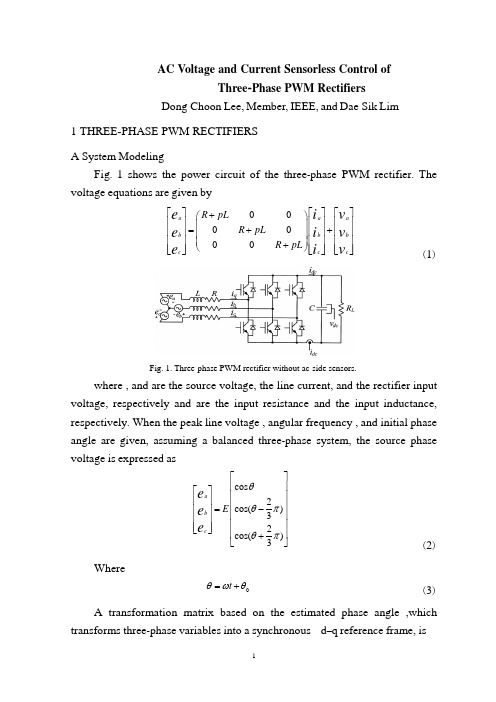
AC Voltage and Current Sensorless Control ofThree -Phase PWM RectifiersDong -Choon Lee, Member, IEEE, and Dae -Sik Lim1 THREE -PHASE PWM RECTIFIERSA System ModelingFig . 1 shows the power circuit of the three -phase PWM rectifier . The voltage equations are given by000000a a a b b b c c c R pL R pL R pL e i v e i v e i v ⎡⎤⎡⎤⎡⎤+⎛⎫⎢⎥⎢⎥⎢⎥ ⎪=++⎢⎥⎢⎥⎢⎥ ⎪⎢⎥⎢⎥⎢⎥ ⎪+⎝⎭⎢⎥⎢⎥⎢⎥⎣⎦⎣⎦⎣⎦ (1)Fig. 1. Three-phase PWM rectifier without ac-side sensors.where , and are the source voltage, the line current, and the rectifier input voltage, respectively and are the input resistance and the input inductance, respectively . When the peak line voltage , angular frequency , and initial phase angle are given, assuming a balanced three -phase system, the source phase voltage is expressed ascos 2cos()32cos()3a b c E e e e θθπθπ⎡⎤⎢⎥⎡⎤⎢⎥⎢⎥⎢⎥=-⎢⎥⎢⎥⎢⎥⎢⎥⎢⎥⎣⎦⎢⎥+⎣⎦ (2) Where0t θωθ=+ (3)A transformation matrix based on the estimated phase angle ,which transforms three -phase variables into a synchronous d –q reference frame, is2322332cos cos()cos()323sin sin()sin()M M M M M M C θθπθπθθπθπ⎛⎫-+ ⎪ ⎪= ⎪++ ⎪⎝⎭ (4)Transforming (1) into the – reference frame using (4)qc qc qc M Mdc dc dc e i v R pL L L R pL e i v ωω⎡⎤⎡⎤⎡⎤+-⎛⎫=+⎢⎥⎢⎥⎢⎥ ⎪+⎝⎭⎣⎦⎣⎦⎣⎦ (5) where p is a differential operator and .M M ωθ=Expressing (5) in a vector notationM e Ri LJi pLi v ω=+++ (6) where,qc dc e e e ⎡⎤=⎢⎥⎣⎦,qc dc i i i ⎡⎤=⎢⎥⎣⎦,qc dc v v v ⎡⎤=⎢⎥⎣⎦,0110J -⎛⎫= ⎪⎝⎭ (7) Taking a transformation of (2) by using (4)cos sin E e E θθ∆⎡⎤=⎢⎥∆⎣⎦ (8) WhereM θθθ∆=- (9)Expressing (6) and (8) in a discrete domain, by approximating the derivative term in (6) by a forward difference [9], respectively,[](1)(1)(1)()(1)(1)M e k Ri k LJi k L i k i k v k T ω-=-+-+--+- (10)cos (1)(1)sin (1)E k e k E k θθ∆-⎡⎤-=⎢⎥-∆-⎣⎦ (11)Where T is the sampling period .Fig. 2. Overall control block diagram.B System ControlThe PI controllers are used to regulate the dc output voltage and the ac input current . For decoupling current control, the cross -coupling terms are compensated in a feed forward -typeand the source voltage is also compensated as a disturbance . For transient responses without overshoot, the anti -windup technique is employed [10]. The overall control block diagram eliminating the source voltage and line current sensors is shown in Fig . 2. The estimation algorithm of source voltages and line currents is described in the following sections .2 PREDICTIVE CURRENT ESTIMATIONThe currents of ()a I k and ()c I k can not be calculated instantly since the calculation time of the DSP is required . To eliminate the delay effect, a state observer can be used . In addition, the state observer provides the filtering effects for the estimated variable .Expressing (5) in a state -space form,x Ax Bu =+ (12) y Cx = (13) where,R L A R L ωω⎛⎫-- ⎪= ⎪ ⎪- ⎪⎝⎭,1010L B L ⎛⎫ ⎪= ⎪ ⎪ ⎪⎝⎭,1001C ⎛⎫= ⎪⎝⎭qc dc i x i ⎡⎤=⎢⎥⎣⎦,qc qc dc dc e v u e v -⎡⎤=⎢⎥-⎣⎦ And y is the output .Transforming (12) and (13) into a discrete domain, respectively,(1)()()X k FX k GU k +=+ (14)()()Y k HX k = (15)where,1111R T T L F R T T L ωω⎛⎫-- ⎪= ⎪ ⎪+- ⎪⎝⎭,00T L G T L ⎛⎫ ⎪= ⎪ ⎪ ⎪⎝⎭Then, the observer equation adding an error correction term to is given by (1)()()(()())X k F X k GU k K Y k Y k +=++- (16) Where K is the observer gain matrix and “^ ” means the estimated quantity, and (1)X k + is the state variable estimated ahead one sampling period . Subtracting (15) from (16), the error dynamic equation of the observer is expressed as(1)[]()rr rr e k F KC e k +=- (17) where ()()()rr e k X k X k =- . Here, it is assumed that the model parameters match well with the real ones . Fig . 3 shows the block diagram of the closed -loop state observer .The state variable error depends only on the initial error and is independent of the input . For (17) to converge to the zero state, the roots of the characteristic equation of (17) should be located within the unit circle .Fig. 3. Closed-loop state observer.Fig. 4. Short pulse region.4EXPERIMENTS AND DISCUSSIONSA. System Hardware ConfigurationFig. 5shows the system hardware configuration. The source voltage is a three-phase,110[V].The input resistance and inductance are0.06Ωand3.3 mH,respectively. The dc link capacitance is2350μF and the switching frequency of the PWM rectifier is3.5kHz.Fig. 5. System hardware configuration.Fig. 6. Dc link currents and corresponding phase currents (in sector V ).The TMS320C31DSP chip operating at33.3MHz is used as a main processor and two12-b A/D converters are used. One of them is dedicated for detecting the dc link current and the other is used for measuring the dc output voltage and the source voltages and currents,where ac side quantities are just measured for performance comparison.One of two internal timers in the DSP is employed to decide the PWM control period and the other is used to determine the dc link current interrupt. Considering the rectifier blanking time of3.5s,A/D conversion time of2.6s, and the other signal delay time,the minimum pulse width is set to10s.A.Experimental ResultsFig. 6shows measured dc link currents and phase currents. In case of sector V of the space vector diagram,the dc link current corresponds to for the switching state of and for that of . Fig. 7(a)shows the raw dc link current before filtering. It has a lot of ringing components due to the resonance of the leakage inductance and the snubber capacitor. When the dc current is sampled at the end point of the active voltage vectors as shown in the figure,the measuring error can be reduced.Fig. 7. Sampling of dc link currents.Fig. 8. Estimated source voltage and current at starting.To reduce this error further,the low pass filter should be employed,of which result is shown in Fig. 7(b). The cut-off frequency of the Butterworth’s second-order filter is112kHz and its delay time is about2sec. Since the ringing frequency is258kHz and the switching frequency is3.5[kHz],the filtered signal without significant delay is acquired.Fig. 8shows the estimated source voltage and current at starting. With the proposed initial estimation strategy,the starting operation is well performed. Fig. 9shows the phaseangle,magnitude,and waveform of the estimated source voltage,which coincide well with measured ones.Fig. 10shows the source voltage and current waveform at unity power factor. Figs. With the estimated quantities for the feedback control,the control performance is satisfactory. The dc voltage variation for load changes will beremarkably decreased if a feedforward control for theload current is added, which is possible without additional cur-rent sensor when the PWM rectifier is combined with the PWM inverter for ac motor drives.Fig. 9. Estimated source voltage in steady state.(a) phase angle (b)magnitude (c) waveform.Fig. 10. Source voltage and current waveforms.(a)estimated (b) measured.4 CONCLUSIONSThis paper proposed a novel control scheme of the PWM rectifiers without employing any ac input voltage and current sensors and with using dc voltage and current sensors only. Reducing the number of the sensors useddecreases the system cost as well as improves the system reliability. The phase angle and the magnitude of the source voltage have been estimated by controlling the deviation between the rectifier current and its model current to be zero. For line current reconstruction,switching states and measured dc link currents were used. To eliminate the effect of the calculation time delay of the microprocessor,the predictive state observer was used. It was shown that the estimation algorithm is robust to the parameter variation. The whole algorithm has been implemented for a proto-type1.5[kV A]PWM rectifier system controlled by TMS320C31DSP. The experimental results have verified that the proposed ac sensor elimination method is feasible.无交流电动势、电流传感器的三相PWM 整流器控制Dong -Choon Lee, Member, IEEE, and Dae -Sik Lim1 三相PWM 整流器A 系统模型图一所示为三相PWM 整流器的主电路,电压等式给出如下:000000a a a b b b c c c R pL R pL R pL e i v e i v e i v ⎡⎤⎡⎤⎡⎤+⎛⎫⎢⎥⎢⎥⎢⎥ ⎪=++⎢⎥⎢⎥⎢⎥ ⎪⎢⎥⎢⎥⎢⎥ ⎪+⎝⎭⎢⎥⎢⎥⎢⎥⎣⎦⎣⎦⎣⎦ (1)图1 无交流传感器三相PWM 整流器其中e ,i 和v 分别是源电压,线电流和整流器的输入电压,R 和L 分别是输入电阻和输入电感。
线性代数 英文讲义
Definition
A matrix is said to be in reduced row echelon form if: ⅰ. The matrix is in row echelon form. ⅱ. The first nonzero entry in each row is the only nonzero entry in its column.
n×n Systems Definition
A system is said to be in strict triangular form if in the kth equation the coefficients of the first k-1 variables are all zero and the coefficient of xk is nonzero (k=1, …,n).
1×n matrix
column vector
x1 x2 X x n
n×1 matrix
Definition
Two m×n matrices A and B are said to be equal if aij=bij for each i and j.
1 1
Matrix Multiplication and Linear Systems
Case 1 One equation in Several Unknows
If we let A (a1 a2 an ) and
Example
x1 x2 1 (a ) x1 x2 3 x 2 x 2 2 1 x1 x2 x3 x4 x5 2 (b) x1 x2 x3 2 x4 2 x5 3 x x x 2 x 3x 2 4 5 1 2 3
MIT公开课-线性代数笔记

目录方程组的几何解释 (2)矩阵消元 (3)乘法和逆矩阵 (4)A的LU分解 (6)转置-置换-向量空间R (8)求解AX=0:主变量,特解 (9)求解AX=b:可解性和解的解构 (10)线性相关性、基、维数 (11)四个基本子空间 (12)矩阵空间、秩1矩阵和小世界图 (13)图和网络 (14)正交向量与子空间 (15)子空间投影 (18)投影矩阵与最小二乘 (20)正交矩阵和Gram-Schmidt正交化 (21)特征值与特征向量 (27)对角化和A的幂 (28)微分方程和exp(At)(待处理) (29)对称矩阵与正定性 (29)正定矩阵与最小值 (31)相似矩阵和若尔当型(未完成) (32)奇异值分解(SVD) (33)线性变换及对应矩阵 (34)基变换和图像压缩 (36)NOTATIONp:projection vectorP:projection matrixe:error vectorP:permutation matrixT:transport signC(A):column spaceN(A):null spaceU:upper triangularL:lower triangularE:elimination matrixQ:orthogonal matrix, which means the column vectors are orthogonalE:elementary/elimination matrix, which always appears in the elimination of matrix N:null space matrix, the “solution matrix” of AX=0R:reduced matrix, which always appears in the triangular matrix, “IF00”I:identity matrixS:eigenvector matrixΛ:eigenvalue matrixC:cofactor matrix关于LINER ALGEBA名垂青史的分析方法:由具象到抽象,由二维到高维。
Math1415_RoucheCapelli

Example 6 Find the rank of
2 3 1 M = 1 −1 3 .
0 4 −4
Answer: We start from the smallest minors:
|2| = 0 ⇒ rank(M ) ≥ 1;
23 1 −1
= 0 ⇒ rank(M ) ≥ 2;
From this definition it is clear that the order of the minors that can be extractedቤተ መጻሕፍቲ ባይዱby A cannot be larger than the minimum between m and n. Suppose indeed that m ≤ n (i.e. there are less rows than columns), it is not possible to obtain a square matrix from A, by cutting rows or columns, whose dimension is larger than m.
There are different methods to solve a linear system (Cramer’s rule, Gaussian elimination, Substitution, ...). We will see that it is possible to determine the number of solutions without necessarily solve it. We need some prerequisites in order to state the main result.
Linear Algebra(线性代数)
一、双语教学班组建学生自愿报名申请。
未修读过“线性代数”,且所在专业的培养方案中“线性代数”为必修课程的学生皆可申请。
申请学生需要有优良的英语基础和数学基础,对英语学习和数学学习有浓厚的兴趣,学习自主性强,已修课程应全部及格。
参加“线性代数”双语教学班的学生在课程考核通过后,不再需要修读中文讲授的“线性代数”课程;未通过者,可参加中文讲授的“线性代数”课程补考。
“线性代数”课程学分数为2.5。
下学期拟组建一个“线性代数”双语教学班,人数约90人。
当报名人数超过90人时,按照平均学分绩点从高到低进行选拔。
学生可以在该班试听两周,可以在开课两周内申请退出该双语教学班。
二、教学及考核课程教学以英文教材为主,强调数学思维训练,并介绍数学软件包Matlab的初步知识。
课程考试采用英文试卷,课程讲授循序渐进增加英语讲授时间。
课堂教学使用英语讲授时间平均超过50%。
该课程考核采用多种方式。
课程总评成绩=课程结束考试成绩(占60%) +课程中期测验(占20%) +平时作业成绩(占10%)+ Project (10%)。
课程期中测验题全部为书中习题。
英语运用能力作为考核指标纳入平时作业成绩的考核。
三、申请时间及上课时间申请参加双语教学班的学生于2012年元月6日(星期五)前将“修读…线性代数‟双语教学课程申请表”(见附表)按班级汇总后交至各学院教务员,学院将报名表汇总后于2012年元月11日前送至教学研究科。
上课时间为2011—2012学年第二学期,第二至第十二周,星期一、星期四晚6:30—8:30。
上课地点另行通知。
四、教材及参考书主要教材:Steven J. Leon,Linear Algebra with Applications(影印版),机械工业出版社,2007.5第七版,定价58元。
主要参考书:S.K.Jain, A.D. Gunawardena,Linear Algebra:An Interactive Approach(影印版),机械工业出版社,2003.7。
第二章 密度泛函理论
If the representation is continuous, one has an integral rather than a sum, for example,
The inner product来自of a ket and a bra is a complex number and satisfies
which is identically (2.1.1). Or, consider the effect of the operator in (2.1.11),
If we use a continuous basis set, (2.1.22) becomes
As another example of the use of (2.1.15), we may prove the formula for the decomposition of a Hermitian operator into its eigenfunctions. Let the kets be the complete set of eigenkets of the linear operator A ,with eigenvalues . Then
A very important type of operator is the projection operator onto a normalized ket
The projection property is manifest when Pt acts on the ket |W) of (2.1.6):
An operator description of a quantum state becomes necessary when the state cannot be represented by a linear superposition of eigenstates of a particular Hamiltonian .This occurs when the system of interest is part of a larger closed system, as for example an individual electron in a manyelectron system, For such a system one does not have a complete Hamiltonian containing only its own degrees of freedom, thereby precluding the wave-function description. A state is said to be pure if it is described by a wave function, mixed if it cannot be described by a wave function.
Linear Algebra & Matrices
• Multiply a row by a non-zero constant • Interchange two rows • Add a multiple of one row to another row
Also known as Gaussian Elimination
…
Simplistic Neural Network
0+0+3 0+0+6 0+0+9
Inverse matrices
• Definition. A matrix A is nonsingular or invertible if there exists a matrix B such that: worked example:
1 -1 1 2 X 2 3 1 3 -1 3 1 3 = 2+1 3 3 -2+ 2 3 3 -1 + 1 3 3 1+2 3 3 = 1 0 0 1
A = 4x3 matrix
21
5 6 74 Matlab notes ( ; End of matrix row ) A = [ 21 5 53 ; 5 34 12 ; 6 33 55 ; 74 27 3 ]
2
34 33 27
53
12 55 3
To extract data: Matrix name( row, column ) Scalar Data Point A( 1 , 2 ) = 2 Row Vector A( 2 , : ) = [ 5 34 12 ] Column Vector A( : , 3 ) = [ 53 ; 12 ; 55 ; 3 ] Smaller Matrix A(2:4,1:2) = [ 5 34 ; 6 33 ; 74 27 ] Another Matrix A( 2:2:4 , 2:3 ) = [ 34 12 ; 27 3 ]
量子力学_基本公式Formulism
e) Two vectors whose inner product is zero are called orthogonal =⇒ a collection of mutually orthogonal normalized vectors, αi |αj = δij , (IV-22) is called an orthonormal set, where δij is the Kronecker delta. f ) Components of vectors can be written as ai = ei |α . (IV-23)
which is uniquely represented by the (ordered) ntuple of its components: |α ↔ (a1, a2 , ..., an ) . v) (IV-17)
It is often easier to work with components than with the abstract vectors themselves. Use whatever method to which you are most comfortable.
iii) There exists a zero (or null) vector, |0 , with the property that |α + |0 = |α , for every vector |α . iv) For every vector |α there is an associated inverse vector (| − α ) such that |α + | − α = |0 . b) (IV-10) (IV-9)
−∞
IV–1
Ordinarydifferentialequation
Ordinary differential equationIn mathematics, an ordinary differential equation (or ODE ) is a relation that contains functions of only one independent variable, and one or more of their derivatives with respect to that variable.A simple example is Newton's second law of motion, which leads to the differential equationfor the motion of a particle of constant mass m . In general, the force F depends upon the position x(t) of the particle at time t , and thus the unknown function x(t) appears on both sides of the differential equation, as is indicated in the notation F (x (t )).Ordinary differential equations are distinguished from partial differential equations, which involve partial derivatives of functions of several variables.Ordinary differential equations arise in many different contexts including geometry, mechanics, astronomy and population modelling. Many famous mathematicians have studied differential equations and contributed to the field,including Newton, Leibniz, the Bernoulli family, Riccati, Clairaut, d'Alembert and Euler.Much study has been devoted to the solution of ordinary differential equations. In the case where the equation is linear, it can be solved by analytical methods. Unfortunately, most of the interesting differential equations are non-linear and, with a few exceptions, cannot be solved exactly. Approximate solutions are arrived at using computer approximations (see numerical ordinary differential equations).The trajectory of a projectile launched from a cannon follows a curve determined by an ordinary differential equation that is derived fromNewton's second law.Existence and uniqueness of solutionsThere are several theorems that establish existence anduniqueness of solutions to initial value problemsinvolving ODEs both locally and globally. SeePicard –Lindelöf theorem for a brief discussion of thisissue.DefinitionsOrdinary differential equationLet ybe an unknown function in x with the n th derivative of y , and let Fbe a given functionthen an equation of the formis called an ordinary differential equation (ODE) of order n . If y is an unknown vector valued function,it is called a system of ordinary differential equations of dimension m (in this case, F : ℝmn +1→ ℝm ).More generally, an implicit ordinary differential equation of order nhas the formwhere F : ℝn+2→ ℝ depends on y(n). To distinguish the above case from this one, an equation of the formis called an explicit differential equation.A differential equation not depending on x is called autonomous.A differential equation is said to be linear if F can be written as a linear combination of the derivatives of y together with a constant term, all possibly depending on x:(x) and r(x) continuous functions in x. The function r(x) is called the source term; if r(x)=0 then the linear with aidifferential equation is called homogeneous, otherwise it is called non-homogeneous or inhomogeneous. SolutionsGiven a differential equationa function u: I⊂ R→ R is called the solution or integral curve for F, if u is n-times differentiable on I, andGiven two solutions u: J⊂ R→ R and v: I⊂ R→ R, u is called an extension of v if I⊂ J andA solution which has no extension is called a global solution.A general solution of an n-th order equation is a solution containing n arbitrary variables, corresponding to n constants of integration. A particular solution is derived from the general solution by setting the constants to particular values, often chosen to fulfill set 'initial conditions or boundary conditions'. A singular solution is a solution that can't be derived from the general solution.Reduction to a first order systemAny differential equation of order n can be written as a system of n first-order differential equations. Given an explicit ordinary differential equation of order n (and dimension 1),define a new family of unknown functionsfor i from 1 to n.The original differential equation can be rewritten as the system of differential equations with order 1 and dimension n given bywhich can be written concisely in vector notation aswithandLinear ordinary differential equationsA well understood particular class of differential equations is linear differential equations. We can always reduce an explicit linear differential equation of any order to a system of differential equation of order 1which we can write concisely using matrix and vector notation aswithHomogeneous equationsThe set of solutions for a system of homogeneous linear differential equations of order 1 and dimension nforms an n-dimensional vector space. Given a basis for this vector space , which is called a fundamental system, every solution can be written asThe n × n matrixis called fundamental matrix. In general there is no method to explicitly construct a fundamental system, but if one solution is known d'Alembert reduction can be used to reduce the dimension of the differential equation by one.Nonhomogeneous equationsThe set of solutions for a system of inhomogeneous linear differential equations of order 1 and dimension ncan be constructed by finding the fundamental system to the corresponding homogeneous equation and one particular solution to the inhomogeneous equation. Every solution to nonhomogeneous equation can then be written asA particular solution to the nonhomogeneous equation can be found by the method of undetermined coefficients or the method of variation of parameters.Concerning second order linear ordinary differential equations, it is well known thatSo, if is a solution of: , then such that:So, if is a solution of: ; then a particular solution of , isgiven by:. [1]Fundamental systems for homogeneous equations with constant coefficientsIf a system of homogeneous linear differential equations has constant coefficientsthen we can explicitly construct a fundamental system. The fundamental system can be written as a matrix differential equationwith solution as a matrix exponentialwhich is a fundamental matrix for the original differential equation. To explicitly calculate this expression we first transform A into Jordan normal formand then evaluate the Jordan blocksof J separately asTheories of ODEsSingular solutionsThe theory of singular solutions of ordinary and partial differential equations was a subject of research from the time of Leibniz, but only since the middle of the nineteenth century did it receive special attention. A valuable but little-known work on the subject is that of Houtain (1854). Darboux (starting in 1873) was a leader in the theory, and in the geometric interpretation of these solutions he opened a field which was worked by various writers, notably Casorati and Cayley. To the latter is due (1872) the theory of singular solutions of differential equations of the first order as accepted circa 1900.Reduction to quadraturesThe primitive attempt in dealing with differential equations had in view a reduction to quadratures. As it had been the hope of eighteenth-century algebraists to find a method for solving the general equation of the th degree, so it was the hope of analysts to find a general method for integrating any differential equation. Gauss (1799) showed, however, that the differential equation meets its limitations very soon unless complex numbers are introduced. Hence analysts began to substitute the study of functions, thus opening a new and fertile field. Cauchy was the first to appreciate the importance of this view. Thereafter the real question was to be, not whether a solution is possible by means of known functions or their integrals, but whether a given differential equation suffices for the definition of a function of the independent variable or variables, and if so, what are the characteristic properties of this function.Fuchsian theoryTwo memoirs by Fuchs (Crelle, 1866, 1868), inspired a novel approach, subsequently elaborated by Thomé and Frobenius. Collet was a prominent contributor beginning in 1869, although his method for integrating a non-linear system was communicated to Bertrand in 1868. Clebsch (1873) attacked the theory along lines parallel to those followed in his theory of Abelian integrals. As the latter can be classified according to the properties of the fundamental curve which remains unchanged under a rational transformation, so Clebsch proposed to classify the transcendent functions defined by the differential equations according to the invariant properties of the corresponding surfaces f = 0 under rational one-to-one transformations.Lie's theoryFrom 1870 Sophus Lie's work put the theory of differential equations on a more satisfactory foundation. He showed that the integration theories of the older mathematicians can, by the introduction of what are now called Lie groups, be referred to a common source; and that ordinary differential equations which admit the same infinitesimal transformations present comparable difficulties of integration. He also emphasized the subject of transformations of contact.A general approach to solve DE's uses the symmetry property of differential equations, the continuous infinitesimal transformations of solutions to solutions (Lie theory). Continuous group theory, Lie algebras and differential geometry are used to understand the structure of linear and nonlinear (partial) differential equations for generating integrable equations, to find its Lax pairs, recursion operators, Bäcklund transform and finally finding exact analytic solutions to the DE.Symmetry methods have been recognized to study differential equations arising in mathematics, physics, engineering, and many other disciplines.Sturm–Liouville theorySturm–Liouville theory is a theory of eigenvalues and eigenfunctions of linear operators defined in terms of second-order homogeneous linear equations, and is useful in the analysis of certain partial differential equations.Software for ODE solving•FuncDesigner (free license: BSD, uses Automatic differentiation, also can be used online via Sage-server [2])•VisSim [3] - a visual language for differential equation solving•Mathematical Assistant on Web [4] online solving first order (linear and with separated variables) and second order linear differential equations (with constant coefficients), including intermediate steps in the solution.•DotNumerics: Ordinary Differential Equations for C# and [5] Initial-value problem for nonstiff and stiff ordinary differential equations (explicit Runge-Kutta, implicit Runge-Kutta, Gear’s BDF and Adams-Moulton).•Online experiments with JSXGraph [6]References[1]Polyanin, Andrei D.; Valentin F. Zaitsev (2003). Handbook of Exact Solutions for Ordinary Differential Equations, 2nd. Ed.. Chapman &Hall/CRC. ISBN 1-5848-8297-2.[2]/welcome[3][4]http://user.mendelu.cz/marik/maw/index.php?lang=en&form=ode[5]/NumericalLibraries/DifferentialEquations/[6]http://jsxgraph.uni-bayreuth.de/wiki/index.php/Differential_equationsBibliography• A. D. Polyanin and V. F. Zaitsev, Handbook of Exact Solutions for Ordinary Differential Equations (2nd edition)", Chapman & Hall/CRC Press, Boca Raton, 2003. ISBN 1-58488-297-2• A. D. Polyanin, V. F. Zaitsev, and A. Moussiaux, Handbook of First Order Partial Differential Equations, Taylor & Francis, London, 2002. ISBN 0-415-27267-X• D. Zwillinger, Handbook of Differential Equations (3rd edition), Academic Press, Boston, 1997.•Hartman, Philip, Ordinary Differential Equations, 2nd Ed., Society for Industrial & Applied Math, 2002. ISBN 0-89871-510-5.•W. Johnson, A Treatise on Ordinary and Partial Differential Equations (/cgi/b/bib/ bibperm?q1=abv5010.0001.001), John Wiley and Sons, 1913, in University of Michigan Historical Math Collection (/u/umhistmath/)• E.L. Ince, Ordinary Differential Equations, Dover Publications, 1958, ISBN 0486603490•Witold Hurewicz, Lectures on Ordinary Differential Equations, Dover Publications, ISBN 0-486-49510-8•Ibragimov, Nail H (1993), CRC Handbook of Lie Group Analysis of Differential Equations Vol. 1-3, Providence: CRC-Press, ISBN 0849344883.External links•Differential Equations (/Science/Math/Differential_Equations//) at the Open Directory Project (includes a list of software for solving differential equations).•EqWorld: The World of Mathematical Equations (http://eqworld.ipmnet.ru/index.htm), containing a list of ordinary differential equations with their solutions.•Online Notes / Differential Equations (/classes/de/de.aspx) by Paul Dawkins, Lamar University.•Differential Equations (/diffeq/diffeq.html), S.O.S. Mathematics.• A primer on analytical solution of differential equations (/mws/gen/ 08ode/mws_gen_ode_bck_primer.pdf) from the Holistic Numerical Methods Institute, University of South Florida.•Ordinary Differential Equations and Dynamical Systems (http://www.mat.univie.ac.at/~gerald/ftp/book-ode/ ) lecture notes by Gerald Teschl.•Notes on Diffy Qs: Differential Equations for Engineers (/diffyqs/) An introductory textbook on differential equations by Jiri Lebl of UIUC.Article Sources and Contributors7Article Sources and ContributorsOrdinary differential equation Source: /w/index.php?oldid=433160713 Contributors: 48v, A. di M., Absurdburger, AdamSmithee, After Midnight, Ahadley,Ahoerstemeier,AlfyAlf,Alll,AndreiPolyanin,Anetode,Ap,Arthena,ArthurRubin,BL,BMF81,********************,Bemoeial,BenFrantzDale,Benjamin.friedrich,BereanHunter,Bernhard Bauer, Beve, Bloodshedder, Bo Jacoby, Bogdangiusca, Bryan Derksen, Charles Matthews, Chilti, Chris in denmark, ChrisUK, Christian List, Cloudmichael, Cmdrjameson, Cmprince, Conversion script, Cpuwhiz11, Cutler, Delaszk, Dicklyon, DiegoPG, Dmitrey, Dmr2, DominiqueNC, Dominus, Donludwig, Doradus, Dysprosia, Ed Poor, Ekotkie, Emperorbma, Enochlau, Fintor, Fruge, Fzix info, Gauge, Gene s, Gerbrant, Giftlite, Gombang, HappyCamper, Heuwitt, Hongsichuan, Ht686rg90, Icairns, Isilanes, Iulianu, Jack in the box, Jak86, Jao, JeLuF, Jitse Niesen, Jni, JoanneB, John C PI, Jokes Free4Me, JonMcLoone, Josevellezcaldas, Juansempere, Kawautar, Kdmckale, Krakhan, Kwantus, L-H, LachlanA, Lethe, Linas, Lingwitt, Liquider, Lupo, MarkGallagher,MathMartin, Matusz, Melikamp, Michael Hardy, Mikez, Moskvax, MrOllie, Msh210, Mtness, Niteowlneils, Oleg Alexandrov, Patrick, Paul August, Paul Matthews, PaulTanenbaum, Pdenapo, PenguiN42, Phil Bastian, PizzaMargherita, Pm215, Poor Yorick, Pt, Rasterfahrer, Raven in Orbit, Recentchanges, RedWolf, Rich Farmbrough, Rl, RobHar, Rogper, Romanm, Rpm, Ruakh, Salix alba, Sbyrnes321, Sekky, Shandris, Shirt58, SilverSurfer314, Ssd, Starlight37, Stevertigo, Stw, Susvolans, Sverdrup, Tarquin, Tbsmith, Technopilgrim, Telso, Template namespace initialisation script, The Anome, Tobias Hoevekamp, TomyDuby, TotientDragooned, Tristanreid, Twin Bird, Tyagi, Ulner, Vadimvadim, Waltpohl, Wclxlus, Whommighter, Wideofthemark, WriterHound, Xrchz, Yhkhoo, 今古庸龍, 176 anonymous editsImage Sources, Licenses and ContributorsImage:Parabolic trajectory.svg Source: /w/index.php?title=File:Parabolic_trajectory.svg License: Public Domain Contributors: Oleg AlexandrovLicenseCreative Commons Attribution-Share Alike 3.0 Unported/licenses/by-sa/3.0/。