双重差分模型幻灯片+-+difference+in+differences+models
双向固定效应和双重差分演示课件

–High: RI ($3.46), NY ($2.75); NJ($2.70)
–Average of $1.32 across states
–Average in tobacco producing states: $0.40
–Average in non-tobacco states, $1.44
–Average price per pack is $5.12
• Beer
–Low (WY, $0.02/gallon)
5
6
Federal taxes
• Cigarettes, $1.01/pack • Wine
– $0.21/750ml bottle for 14% alcohol or less – $0.31/750ml bottle for 14 – 21% alcohol
for permanent differences between groups • vt – time fixed effects. Impacts common to all groups but vary by year • εit -- idiosyncratic error
3
Excises taxes on poor health
Taxes now an integral part of antismoking campaigns
• Key component of ‘Master Settlement’
• Beer, $0.02 a can • Liquor, $13.50 per 100 proof gallon (50% alcohol),
or, $2.14/750 ml bottle of 80 proof liquor • Total taxes on cigarettes are such that in NYC,
《教学分析》-DID双重差分回归
Y
Yc1 Yt1 Yc2 Yt2
t1
Treatment effect= (Yt2-Yt1) – (Yc2-Yc1)
control treatment t2
time
Difference in Difference
Before Change
Group 1 Yt1 (Treat)
Group 2 Yc1 (Control)
– Ait =1 in the periods when treatment occurs – TitAit -- interaction term, treatment states after
the intervention
• Yit = β0 + β1Tit + β2Ait + β3TitAit + εit
• Only two periods • Intervention will occur in a group of
observations (e.g. states, firms, etc.)
• Three key variables
– Tit =1 if obs i belongs in the state that will eventually be treated
• Cross-sectional and time series data • One group is ‘treated’ with intervention • Have pre-post data for group receiving
intervention • Can examine time-series changes but,
• In this example, Y falls by Yc2-Yc1 even without the intervention
PSM-DID分析ppt课件
(1)基数小,增长快(一张白纸可以画出更美丽的画卷) (2)税收优惠政策对西部地区的增长具有促进作用,效果
将越来越微弱; (3)西部地区与发达地区之间的区域差距仍在继续扩大。
15
政策陷阱效应
• 优惠政策构成了西部地区经济增长的驱动力,但 其增长对能源、资源开发的依赖度很高;由于体 制弊端和配套政策缺失,会造成地方政府的短视 行为,容易忽视人才和技术要素,弱化社会制度 和软环境构建。
PSM—DID及其应用
1
1、介绍PSM-DID方法 2、分析论文
——西部大开发是增长驱动还是政策陷阱
3、stata操作过程
2
双重差分法
• 双重差分(difference in differences,DID)嘛,就是 差分两次。
• 一种专门用于分析政策效果的计量方法。 • 将制度变迁和新政策视为一次外生于经济系统的“自然实
大开发之前的处理组、西部大开发之后的处理组、西部大开发之前的 控制组和西部大开发之后的控制组。
• du=1代表西部地区的地级市,du=0代表其他地区的地级市,dt= 0代表西部大开发之前的年份,dt=1代表西部大开发之后的年份。
• 下标i和t分别代表第i个地级市和第t年,Z代表一系列控制变量, e为随机扰动项,被解释变量Y度量经济增长,具体指标包括人均实 际GDP和实际GDP的对数值。
城市的GDP增长率,Yi Yi1 Yi0
• (2)求处理效应:
1
1
Y N1
(Yi Di 1) N2
(Yi Di 0)
修建铁路对城市经济的促进作用 6
修建铁路对沿线城市经济的影响
• 可以换一个写法 • T=1,建铁路之后 • T=0,建铁路之前 • Treated代表在某一期,某一类城市是不是建了铁路。第零
双重差分模型幻灯片+-+difference+in+differences+models

Y Yc1 Treatment effect= (Yt2-Yt1) – (Yc2-Yc1)
Yc2 Yt1
control Yt2 treatment t1 t2 Treatment Effect
time
11
• In contrast, what is key is that the time trends in the absence of the intervention are the same in both groups • If the intervention occurs in an area with a different trend, will under/over state the treatment effect • In this example, suppose intervention occurs in area with faster falling Y
17
• ui is a state effect • vt is a complete set of year (time) effects • Analysis of covariance model • Yit = β0 + β3 TitAit + ui + λt + εit
18
What is nice about the model
3
Y True effect = Yt2-Yt1 Estimated effect = Yb-Ya Yt1 Ya Yb Yt2
t1
ti
t2
time
4
• Intervention occurs at time period t1 • True effect of law
双重差分模型的平行趋势假定如何检验? coefplot命令来告诉你(一)
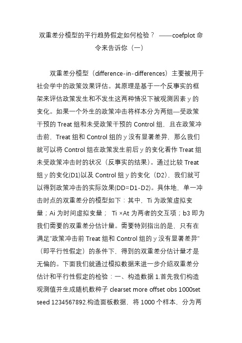
双重差分模型的平行趋势假定如何检验?——coefplot命令来告诉你(一)双重差分模型(difference-in-differences)主要被用于社会学中的政策效果评估。
其原理是基于一个反事实的框架来评估政策发生和不发生这两种情况下被观测因素y的变化。
如果一个外生的政策冲击将样本分为两组—受政策干预的Treat组和未受政策干预的Control组,且在政策冲击前,Treat组和Control组的y没有显著差异,那么我们就可以将Control组在政策发生前后y的变化看作Treat组未受政策冲击时的状况(反事实的结果)。
通过比较Treat组y的变化(D1)以及Control组y的变化(D2),我们就可以得到政策冲击的实际效果(DD=D1-D2)。
具体地,单一冲击时点的双重差分的模型如下:其中,Ti为政策虚拟变量;Ai为时间虚拟变量;Ti ×At为两者的交互项;b3即为我们需要的双重差分估计量。
需要特别指出的是,只有在满足”政策冲击前Treat 组和Control组的y没有显著差异”(即平行性假定)的条件下,得到的双重差分估计量才是无偏的。
下面我们就通过模拟数据来进一步介绍双重差分估计和平行性假定的检验:一、构造数据1.首先我们构造观测值并生成随机数种子clearset more offset obs 1000set seed 1234567892.构造面板数据,将1000个样本,分为两组:实验组(Treat==1),对照组(Treat==0)gen Treat=(uniform()3.根据随机数构造公司-年度数据bysort Treat: gen intgroup=uniform()*90+Treat*90+1bysort group: genyear=2016-_n+14.假定2012年,实验组(Treat==1)公司受到一个外生政策冲击gen Post=(year>=2012)5.模拟被解释变量y,控制变量x1,x2gen y=ln(1+uniform()*100)replace y=y + ln(uniform()*10+rnormal()*3) if Treat==1 & Post==1 gen x1=rnormal()*3gen x2=rnormal()+uniform()我们可以看到,公司id(group)、年份(year)、分组标识(Treat)、冲击发生标识(Post)、被解释变量(y)以及控制变量(x1, x2)已经生成。
双重差分模型幻灯片
unsure how much of the change is due to secular changes
2
Y
Yt1 Ya Yb Yt2
True effect = Yt2-Yt1 Estimated effect = Yb-Ya
6
Difference in Difference
Before Change
Group 1 Yt1 (Treat)
Group 2 Yc1 (Control)
Difference
After Change Yt2
Yc2
Difference
ΔYt = Yt2-Yt1 ΔYc =Yc2-Yc1 ΔΔY ΔYt – ΔYc
• Key concept: can control for the fact that the intervention is more likely in some types of states
5
Three different presentations
• Tabular • Graphical • Regression equation
• Application of two-way fixed effects model
1
Problem set up
• Cross-sectional and time serintervention • Have pre-post data for group receiving
t1
ti
t2
time
3
• Intervention occurs at time period t1 • True effect of law
二重差分法分析(DID)
二重差分法分析(DID)双重差分模型(difference-in-differences)主要被用于社会学中的政策效果评估。
其原理是基于一个反事实的框架来评估政策发生和不发生这两种情况下被观测因素y的变化。
如果一个外生的政策冲击将样本分为两组—受政策干预的Treat组和未受政策干预的Control 组,且在政策冲击前,Treat组和Control组的y没有显著差异,那么我们就可以将Control组在政策发生前后y的变化看作Treat组未受政策冲击时的状况(反事实的结果)。
通过比较Treat组y的变化(D1)以及Control组y的变化(D2),我们就可以得到政策冲击的实际效果(DD=D1-D2)。
双重差分法,英文名Differences-in-Differences,别名“倍差法”,小名“差中差”。
作为政策效应评估方法中的一大利器,双重差分法受到越来越多人的青睐,概括起来有如下几个方面的原因:(1)可以很大程度上避免内生性问题的困扰:政策相对于微观经济主体而言一般是外生的,因而不存在逆向因果问题。
此外,使用固定效应估计一定程度上也缓解了遗漏变量偏误问题。
(2)传统方法下评估政策效应,主要是通过设置一个政策发生与否的虚拟变量然后进行回归,相较而言,双重差分法的模型设置更加科学,能更加准确地估计出政策效应。
(3)双重差分法的原理和模型设置很简单,容易理解和运用,并不像空间计量等方法一样让人望而生畏。
(4)尽管双重差分法估计的本质就是面板数据固定效应估计,但是DID听上去或多或少也要比OLS、FE之流更加“时尚高端”,因而DID的使用一定程度上可以满足“虚荣心”。
在细致介绍DID之前首先强调一点,一般而言,DID仅适用于面板数据,因此在只有截面数据时,还是不要浪费心思在DID上了。
不过,事无绝对,在某些特殊的情景下,截面数据通过巧妙的构造也是可以运用DID的,大神Duflo曾经就使用截面数据和DID研究了南非的养老金计划项目对学前儿童健康的影响,感兴趣的可以去搜搜大神的文章。
DID双重差分回归课件
(return to this in the regression equation)
• Cross section and time fixed effects
• Use time series of untreated group to establish what would have occurred in the absence of the intervention
• Key concept: can control for the fact that the intervention is more likely in some types of states
• If the intervention occurs in an area with a different trend, will under/over state the treatment effect
• In this example, suppose intervention occurs in area with faster falling Y
Difference in Difference Models
DID双重差分回归
1
What is DID
• How can we estimate the effects of higher education reform in China?
• Yang and Chen (2009)
DID双重差分回归
Y
Estimated treatment Yc1
Yt1
Yc2
True treatment effect
control
Yt2 treatment t1 t2
True Treatment Effect
time
12
Basic Econometric Model
• Data varies by
– state (i) – time (t) – Outcome is Yit
• This is captured by the inclusion of the state/time effects – allows covariance between
– ui and TitAit – λt and TitAit
18
• Group effects
– Capture differences across groups that are constant over time
Difference in Difference Models
1
What is DID
• How can we estimate the effects of higher education reform in China? • Yang and Chen (2009)
2
Problem set up
• Yit = β0 + β1Tit + β2Ait + β3TitAit + εit
14
Yit = β0 + β1Tit + β2Ait + β3TitAit + εit
Before Change
Group 1 (Treat) Group 2 (Control) Difference β0 + β1 β0
PSM-DID分析ppt课件
修建铁路对沿线城市经济的影响
• 为了解决以上问题,我们需要观察到至少两期, 第一期是建铁路之前, T=0;第二期是建铁路之 后, T=1 。
• 设穿过Di=1,否则Di=0。
• 两次差分,(1)先求出在修建铁路前后每一个
期肯定没有建铁路,第一期只有Di=1的城市建了铁路。 基 本模型为:
Yit β0 β1Di β2T β3 (Di T ) β4 Xit εit
• 对时间差分: Yi β2 β3Di εit • 再次差分: Y β3 εit
• 所以实际做的时候,可以直接跑这个式子的回归, 得到的交乘项的系数就是所要估计的处理效应。
• 如果我们简单地将是否执行了某项事件作为虚拟
变量,而对总体进行回归的话,参数估计就会产
生偏误,因为在这样的情况下,我们只观察到了
某一个对象他因为发生了某一事件后产生的表现,
并且拿这种表现去和另一些没有发生这件事情的
其他对象去做比较。这样的比较显然是不科学的,
因为比较的基础并不同。
4
修建铁路对沿线城市经济的影响
PSM—DID及其应用
1
1、介绍PSM-DID方法 2、分析论文
——西部大开发是增长驱动还是政策陷阱
3、stata操作过程
2
双重差分法
• 双重差分(difference in differences,DID)嘛,就是 差分两次。
• 一种专门用于分析政策效果的计量方法。 • 将制度变迁和新政策视为一次外生于经济系统的“自然实
• 现在要修一条铁路,铁路是条线,所以必然会有 穿过的城市和没有被穿过的城市;
- 1、下载文档前请自行甄别文档内容的完整性,平台不提供额外的编辑、内容补充、找答案等附加服务。
- 2、"仅部分预览"的文档,不可在线预览部分如存在完整性等问题,可反馈申请退款(可完整预览的文档不适用该条件!)。
- 3、如文档侵犯您的权益,请联系客服反馈,我们会尽快为您处理(人工客服工作时间:9:00-18:30)。
• This is captured by the inclusion of the state/time effects – allows covariance between
– ui and TitAit – λt and TitAit
19
• Group effects
– Capture differences across groups that are constant over time
2
Problem set up
• Cross-sectional and time series data • One group is „treated‟ with intervention • Have pre-post data for group receiving intervention • Can examine time-series changes but, unsure how much of the change is due to secular changes
• Many periods • Intervention will occur in a group of states but at a variety of times
17
• ui is a state effect • vt is a complete set of year (time) effects • Analysis of covariance model
• Yit = β0 + β1Tit + β2Ait + β3TitAit + εit
15
Yit = β0 + β1Tit + β2Ait + β3TitAit + εit
Before Change
Group 1 (Treat) Group 2 (Control) Difference β0 + β1 β0
After Change
Yt2 Yc2
Difference ΔYt = Yt2-Yt1 ΔYc =Yc2-Yc1 ΔΔY ΔYt – ΔYc
8
Y Treatment effect= (Yt2-Yt1) – (Yc2-Yc1) Yc1
Yt1
Yc2
Yt2
control treatment t1 t2
time
24
Solution
• Quasi experiment in KY and MI • Increased the earnings cap
– Increased benefit for high-wage workers
• (Treatment)
– Did nothing to those already below original cap (comparison)
• Compare change in duration of spell before and after change for these two groups
25
26
27
Model
• Yit = duration of spell on WC • Ait = period after benefits hike • Hit = high earnings group (Income>E3)
6
Three different presentations
• Tabular • Graphical • Regression equation
7
Difference in Difference
Before Change
Group 1 (Treat) Group 2 (Control) Difference Yt1 Yc1
22
• Concern:
– Moral hazard. Benefits will discourage return to work
• Empirical question: duration/benefits gradient • Previous estimates
– Regress duration (y) on replaced wages (x)
• Yit = β0 + β1Hit + β2Ait + β3AitHit + β4Xit‟ + εit • Diff-in-diff estimate is β3
28
29
Questions to ask?
• What parameter is identified by the quasiexperiment? Is this an economically meaningful parameter? • What assumptions must be true in order for the model to provide and unbiased estimate of β3? • Do the authors provide any evidence supporting these assumptions?
After Change
Difference
β0+ β1+ β2+ β3 ΔYt = β2 + β3 β0 + β2 ΔYc = β2 ΔΔY = β3
16
ห้องสมุดไป่ตู้
More general model
• Data varies by
– state (i) – time (t) – Outcome is Yit
12
Y
Estimated treatment Yc1
Yt1
Yc2
True treatment effect
control
Yt2 treatment t1 t2
True Treatment Effect
time
13
Basic Econometric Model
• Data varies by
– state (i) – time (t) – Outcome is Yit
Difference in Difference Models
Bill Evans Spring 2008
1
Difference in difference models
• Maybe the most popular identification strategy in applied work today • Attempts to mimic random assignment with treatment and “comparison” sample • Application of two-way fixed effects model
• Premiums
– Paid by firms – Function of previous claims and wages paid
• Benefits -- % of income w/ cap
21
• Typical benefits schedule
– Min( pY,C) – P=percent replacement – Y = earnings – C = cap – e.g., 65% of earnings up to $400/month
• Use time series of untreated group to establish what would have occurred in the absence of the intervention • Key concept: can control for the fact that the intervention is more likely in some types of states
3
Y True effect = Yt2-Yt1 Estimated effect = Yb-Ya
Yt1
Ya Yb Yt2
t1
ti
t2
time
4
• Intervention occurs at time period t1 • True effect of law
– Ya – Yb
• Only have data at t1 and t2
– If using time series, estimate Yt1 – Yt2
• Solution?
5
Difference in difference models
• Basic two-way fixed effects model
– Cross section and time fixed effects
• Year effects
– Capture differences over time that are common to all groups
20
Meyer et al.
• Workers‟ compensation
– State run insurance program – Compensate workers for medical expenses and lost work due to on the job accident
• Yit = β0 + β3 TitAit + ui + λt + εit
18
What is nice about the model
• Suppose interventions are not random but systematic
– Occur in states with higher or lower average Y – Occur in time periods with different Y‟s