2014美赛B题论文
2014 数学建模美赛B题
PROBLEM B: College Coaching LegendsSports Illustrated, a magazine for sports enthusiasts, is looking for the “best all time college coach”male or female for the previous century. Build a mathematical model to choosethe best college coach or coaches (past or present) from among either male or female coaches in such sports as college hockey or field hockey, football, baseball or softball, basketball, or soccer. Does it make a difference which time line horizon that you use in your analysis, i.e., does coaching in 1913 differ from coaching in 2013? Clearly articulate your metrics for assessment. Discuss how your model can be applied in general across both genders and all possible sports. Present your model’s top 5 coaches in each of 3 different sports.In addition to the MCM format and requirements, prepare a 1-2 page article for Sports Illustrated that explains your results and includes a non-technical explanation of your mathematical model that sports fans will understand.问题B:大学教练的故事体育画报,为运动爱好者杂志,正在寻找上个世纪堪称“史上最优秀大学教练”的男性或女性。
对创意平板折叠桌的最优化设计-2014年数学建模国赛B题
承诺书我们仔细阅读了《全国大学生数学建模竞赛章程》和《全国大学生数学建模竞赛参赛规则》(以下简称为“竞赛章程和参赛规则”,可从全国大学生数学建模竞赛网站下载)。
我们完全明白,在竞赛开始后参赛队员不能以任何方式(包括电话、电子邮件、网上咨询等)与队外的任何人(包括指导教师)研究、讨论与赛题有关的问题。
我们知道,抄袭别人的成果是违反竞赛章程和参赛规则的,如果引用别人的成果或其他公开的资料(包括网上查到的资料),必须按照规定的参考文献的表述方式在正文引用处和参考文献中明确列出。
我们郑重承诺,严格遵守竞赛章程和参赛规则,以保证竞赛的公正、公平性。
如有违反竞赛章程和参赛规则的行为,我们将受到严肃处理。
我们授权全国大学生数学建模竞赛组委会,可将我们的论文以任何形式进行公开展示(包括进行网上公示,在书籍、期刊和其他媒体进行正式或非正式发表等)。
我们参赛选择的题号是(从A/B/C/D中选择一项填写): B我们的报名参赛队号为(8位数字组成的编号):27027006所属学校(请填写完整的全名):宝鸡文理学院参赛队员(打印并签名) :指导教师或指导教师组负责人(打印并签名):李晓波(论文纸质版与电子版中的以上信息必须一致,只是电子版中无需签名。
以上内容请仔细核对,提交后将不再允许做任何修改。
如填写错误,论文可能被取消评奖资格。
)日期: 2014年 09 月 15 日赛区评阅编号(由赛区组委会评阅前进行编号):编号专用页赛区评阅编号(由赛区组委会评阅前进行编号):全国统一编号(由赛区组委会送交全国前编号):全国评阅编号(由全国组委会评阅前进行编号):对创意平板折叠桌的最优化设计摘要本文主要研究了创意平板折叠桌的相关问题。
对于问题一,首先,我们根据所提供的已知尺寸的长方形平板和桌面形状,桌高的要求,以圆桌面中心作为原点建立了相应的空间直角坐标系,分别求出了各个桌腿的长度,根据在折叠过程中,钢筋穿过的每个点距离桌面的高度相同这一性质,利用MATLAB程序计算出了每根木棒卡槽的长度和桌脚底端每个点的坐标,其中卡槽长度依次为(从最外侧开始,单位:cm):0、 4.3564、7.663、10.3684、12.5926、14.393、15.8031、16.8445、17.5314、17.8728,并且根据底端坐标拟合出了桌脚边缘线的方程并进行了检验。
2014研究生数学建模B题优秀论文
三 符号说明
r
r
k
目标径向距离 目标方位角 目标俯仰角 雷达极坐标下测距误 差 雷达极坐标下方位角 误差 雷达极坐标下俯仰角 误差 雷达在地球直角坐标 下 x 轴上的标准差 雷达在地球直角坐标 下 y 轴上的标准差 雷达在地球直角坐标 下 z 轴上的标准差 目标的运动状态
-3-
一 问题重述
目标跟踪是指根据雷达等传感器所获得的对目标的测量信息, 连续地对目标 的运动状态进行估计,进而获取目标的运动态势及意图。目标机动则是指目标的 速度大小和方向在短时间内发生变化,通常采用加速度作为衡量指标。目标跟踪 与目标机动是“矛”与“盾”的关系。因此,引入了目标机动时雷达如何准确跟踪的 问题。 机动目标跟踪的难点在于以下几个方面:(1) 描述目标运动的模型,即目标 的状态方程难于准确建立。通常情况下跟踪的目标都是非合作目标,目标的速度 大小和方向如何变化难于准确描述; (2) 传感器自身测量精度有限加之外界干 扰,传感器获得的测量信息,如距离、角度等包含一定的随机误差,用于描述传 感器获得测量信息能力的测量方程难于完全准确反映真实目标的运动特征; (3) 当存在多个机动目标时,除了要解决(1)、(2)两个问题外,还需要解决测量信息 属于哪个目标的问题,即数据关联。由于以上多个挑战因素以及目标机动在战术 上主动的优势,机动目标跟踪已成为近年来跟踪理论研究的热点和难点[1]。 目标跟踪处理流程通常可分为航迹起始、点迹航迹关联(数据关联)、航迹 滤波等步骤。 另外, 不同类型目标的机动能力不同。 因此, 在对机动目标跟踪时, [2] 必须根据不同的目标类型选择相应的跟踪模型 。 根据题目提供的 3 组机动目标测量数据,本文拟解决以下问题: 问题一 根据附件中的 Data1.txt 数据,分析目标机动发生的时间范围,并 统计目标加速度的大小和方向。建立对该目标的跟踪模型,并利用多个雷达的 测量数据估计出目标的航迹。鼓励在线跟踪。 问题二 附件中的 Data2.txt 数据对应两个目标的实际检飞考核的飞行包线 (检飞:军队根据国家军标规则设定特定的飞行路线用于考核雷达的各项性能 指标,因此包线是有实战意义的)。请完成各目标的数据关联,形成相应的航 迹,并阐明你们所采用或制定的准则(鼓励创新)。如果用序贯实时的方法实 现更具有意义。若出现雷达一段时间只有一个回波点迹的状况,怎样使得航迹 不丢失?请给出处理结果。 问题三 根据附件中 Data3.txt 的数据,分析空间目标的机动变化规律(目标 加速度随时间变化)。若采用第 1 问的跟踪模型进行处理,结果会有哪些变化? 问题四 请对第 3 问的目标轨迹进行实时预测,估计该目标的着落点的坐 标,给出详细结果,并分析算法复杂度。 问题五 Data2.txt 数据中的两个目标已被雷达锁定跟踪。 在目标能够及时了 解是否被跟踪,并已知雷达的测量精度为雷达波束宽度为 3° ,即在以雷达为锥 顶,雷达与目标连线为轴,半顶角为 1.5° 的圆锥内的目标均能被探测到;雷达 前后两次扫描时间间隔最小为 0.5s。为应对你们的跟踪模型,目标应该采用怎 样的有利于逃逸的策略与方案?反之为了保持对目标的跟踪,跟踪策略又应该 如何相应地变换?
2014年美国大学生数学建模竞赛A题论文综述
数学建模综述2014年美国大学生数学建模竞赛A题论文综述我们小组精读两篇14年美赛A题论文,选择了其中一篇来进行学习,总结。
1、问题分析The Keep-Right-Except-To-Pass Rule除非超车否则靠右行驶的交通规则问题:建立数学模型来分析这条规则在低负荷和高负荷状态下的交通路况的表现。
这条规则在提升车流量的方面是否有效?如果不是,提出能够提升车流量、安全系数或其他因素的替代品(包括完全没有这种规律)并加以分析。
在一些国家,汽车靠左形式是常态,探讨你的解决方案是否稍作修改即可适用,或者需要一些额外的需要。
最后,以上规则依赖于人的判断,如果相同规则的交通运输完全在智能系统的控制下,无论是部分网络还是嵌入使用的车辆的设计,在何种程度上会修改你前面的结果论文:基于元胞自动机和蒙特卡罗方法,我们建立一个模型来讨论“靠右行”规则的影响。
首先,我们打破汽车的运动过程和建立相应的子模型car-generation的流入模型,对于匀速行驶车辆,我们建立一个跟随模型,和超车模型。
然后我们设计规则来模拟车辆的运动模型。
我们进一步讨论我们的模型规则适应靠右的情况和,不受限制的情况, 和交通情况由智能控制系统的情况。
我们也设计一个道路的危险指数评价公式。
我们模拟双车道高速公路上交通(每个方向两个车道,一共四条车道),高速公路双向三车道(总共6车道)。
通过计算机和分析数据。
我们记录的平均速度,超车取代率、道路密度和危险指数和通过与不受规则限制的比较评估靠右行的性能。
我们利用不同的速度限制分析模型的敏感性和看到不同的限速的影响。
左手交通也进行了讨论。
根据我们的分析,我们提出一个新规则结合两个现有的规则(靠右的规则和无限制的规则)的智能系统来实现更好的的性能。
该论文在一开始并没有作过多分析,而是一针见血的提出了自己对于这个问题的做法。
由于题目给出的背景只有一条交通规则,而且是题目很明确的提出让我们建立模型分析。
2014MCM-B优秀论文
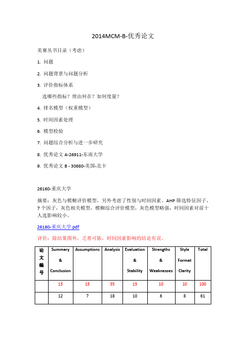
2014MCM-B-优秀论文美赛丛书目录(考虑)1. 问题2. 问题背景与问题分析3. 评价指标体系选哪些指标?理由何在?如何度量?4. 排名模型(权重模型)5. 时间因素处理6. 模型检验7. 问题综合分析与进一步研究8. 优秀论文A-26911-东南大学9. 优秀论文B - 30680-美国-北卡26160-重庆大学摘要:灰色与模糊评价模型,另外考虑了性别与时间因素。
AHP筛选特征因子,7个因子,灰色相关模型,模糊综合评价模型,灰色模型略强,时间因素对前十人选影响较小。
26160-重庆大学.pdf评价:除结果图外,乏善可陈,时间因素影响的结论有误。
26636-外经贸大学摘要:灰色相关模型,依据专家意见选择了四个评价指标:NCAA冠军,Pct,胜场数,教练报酬。
模糊相容矩阵确定各个评价指标的权值,结果与ESPN作比较。
最后讨论了时间因素,发现规律:“从前”的教练的胜率要远远高于“现在”的教练,但其他三个指标所受到的影响很小。
引入滑动平均方法,将时间因素纳入胜率计算模型中,这是本文的一个亮点。
Shannon熵用于评价稳定性。
讨论了参数敏感性。
便利与普适是我们模型的最大优点,但存在指标选择的主观性。
26636-外经贸.pdf评价:指标体系以及评价模型一般,有点投机,时间因素讨论、模型结果检验以及敏感性检验是亮点,结果对比表达清晰明了,可信度高。
缺假设与“conclusion”,是硬伤。
26911-东南大学三阶段全面评价模型,指标体系(胜率,稳定性,获得冠军数量,个人报酬,点击率,个人荣誉,职业联赛排名),谷歌趋势统计方法,线性拟合方法,加权和模型,AHP+最大熵模型,灰色相关分析,综合排名26911-东南大学.pdf评价:非常全面,思路很清晰,表达很简洁,值得效仿。
具体说:指标意义讨论充分;指标取值实用、合理;时间因素考虑到位;权重确定有技术含量;结果表达清晰;文章节奏把握好。
如果按更高标准衡量,第二种权重体系中GRA的作用不大显著。
2014年美赛数学建模A题翻译版论文

2014年美赛数学建模A题翻译版论文D流入模型,或vehicle-generation模型,模拟了随机到达高速公路的入口处的车辆。
对于每一个车道,前六个细胞在元胞自动机中设置为vehicle-generation区域。
我们假设每辆车的到达服从二项概率分布。
让ts表示采样时间间隔和N表示在ts时间内车辆的总数。
然后N可以近似服从泊松概率分布。
让Pt(N)表示N的可能性,于是我们有ts表示在一秒,我们可以分配N的期望的值的范围从0到3.6。
N作为在每一秒中到达的总车辆,N的期望能有效地反映交通状况。
λ越小,交通越轻松。
因此我们能够模拟不同流量条件下,交通的轻或重,通过分配相应的值λ。
λ的值设定后,我们得到了进入高速公路的车辆模拟每一秒的随机号码。
每个车道然后随机分配进入。
我们的车辆模型支持两种不同的速度范围, 假设所有车辆的初始速度设置为20 m / s。
这种做法带来了简化而不削弱结果。
这是因为由于交通密度控制和加速度的分布概率的引入,所有车辆的速度往往是一个值。
当交通密度低,车辆可以自由加速到最大速度,而不用担心冲突,因此收敛速度在允许的最高速度而不用担心撞车。
当交通密度高,所有的通道将充满车辆,交通流的速度是由车道上速度最慢的车决定,因此收敛速度是在较低的速度限制。
经过初步分析,收敛速度模型稍后将合理的实现。
利用泊松概率分布使流入模型接近现实和实用。
由于收敛趋势,一样的初速度在不改变的情况下就能得到简化。
2.3 Vehicle-Following Model美国联邦公路管理局的部门定义司机的反应时间PIEV时间。
PIEV时间由四部分组成:•感知过程:司机在驾驶环境中感知的变化。
•理解过程:司机分析关于变化的信息。
•评估过程:司机决定根据他的驾驶行为分析。
•意志过程:司机执行驾驶行为我们应用PIEV在匀速行驶模型和超车模型。
在每次循环中,我们首先获得每辆车的速度和位置,计算差距,然后确定驾驶行为(无论继续或改变车道超车后)。
2014建模美赛B题
For office use onlyT1________________ T2________________ T3________________ T4________________ Team Control Number27820Problem ChosenBFor office use onlyF1________________F2________________F3________________F4________________ 2014Mathematical Contest in Modeling (MCM/ICM) Summary Sheet(Attach a copy of this page to your solution paper.)Research on Choosing the Best College Coaches Based on Data Envelopment AnalysisSummaryIn order to get the rank of coaches in differ ent sports and look for the ―best all time college coach‖ male or female for the previous century, in this paper, we build a comprehensive evaluation model for choosing the best college coaches based on data envelopment analysis. In the established model, we choose the length of coaching career, the number of participation in the NCAA Games, and the number of coaching session as the input indexes, and choose the victory ratio of games, the number of victory session and the number of equivalent champion as the output indexes. In addition, each coach is regarded as a decision making unit (DMU).First of all, with the example of basketball coaches, the relatively excellent basketball coaches are evaluated by the established model. By using LINGO software, the top 5 coaches are obtained as follows: Joe B. Hall, John Wooden, John Calipari, Adolph Rupp and Hank Iba.Secondly, the year 1938 is chosen as a time set apart to divide the time line into two parts. And then, basketball coaches are still taken as an example to evaluate the top 5 coaches used the constructed model in those two parts, respectively. The evaluated results are shown as: Doc Meanwell, Francis Schmidt, Ralph Jones, E.J. Mather, Harry Fisher before 1938, and Joe B. Hall, John Wooden, John Calipari, Adolph Rupp and Hank Iba after 1938. These results are accordant with those best coaches that were universally acknowledged by public. It suggests that the model is valid and effective. As a consequence, it can be applied in general across both genders and all possible sports.Thirdly, just the same as basketball coaches, football and field hockey coaches are also studied by using the model. After the calculation, the top 5 co aches of football’s results are as follows: Phillip Fulmer, Tom Osborne, Dan Devine, Bobby Bowden and Pat Dye, and field hockey’s are Fred Shero, Mike Babcock, Claude Julien, Joel Quenneville and Ken Hitchcock.Finally, although the top 5 coaches in each of 3 different sports have been chosen, the above-mentioned model failed to sort these coaches. Therefore, the super- efficiency DEA model is introduced to solve the problem. This model not only can evaluate the better coaches but also can rank them. As a result, we can choose the ―best all time college coach‖ from all the coaches easily.Type a summary of your results on this page. Do not includethe name of your school, advisor, or team members on this page.Research on Choosing the Best College Coaches Based on DataEnvelopment AnalysisSummaryI n order to get the rank of coaches in different sports and look for the ―best all time college coach‖ male or female for the previous century, in this paper, we build a comprehensive evaluation model for choosing the best college coaches based on data envelopment analysis. In the established model, we choose the length of coaching career, the number of participation in the NCAA Games, and the number of coaching session as the input indexes, and choose the victory ratio of games, the number of victory session and the number of equivalent champion as the output indexes. In addition, each coach is regarded as a decision making unit (DMU).First of all, with the example of basketball coaches, the relatively excellent basketball coaches are evaluated by the established model. By using LINGO software, the top 5 coaches are obtained as follows: Joe B. Hall, John Wooden, John Calipari, Adolph Rupp and Hank Iba.Secondly, the year 1938 is chosen as a time set apart to divide the time line into two parts. And then, basketball coaches are still taken as an example to evaluate the top 5 coaches used the constructed model in those two parts, respectively. The evaluated results are shown as: Doc Meanwell, Francis Schmidt, Ralph Jones, E.J. Mather, Harry Fisher before 1938, and Joe B. Hall, John Wooden, John Calipari, Adolph Rupp and Hank Iba after 1938. These results are accordant with those best coaches that were universally acknowledged by public. It suggests that the model is valid and effective. As a consequence, it can be applied in general across both genders and all possible sports.Thirdly, just the same as basketball coaches, football and field hockey coaches are also studied by using the model. After the calculation, the top 5 coaches of football’s results are as follows: Phillip Fulmer, Tom Osborne, Dan Devine, Bobby Bowden and Pat Dye, and field hockey’s are Fred Shero, Mike Babcock, Claude Julien, Joel Quenneville and Ken Hitchcock.Finally, although the top 5 coaches in each of 3 different sports have been chosen, the above-mentioned model failed to sort these coaches. Therefore, the super- efficiency DEA model is introduced to solve the problem. This model not only can evaluate the better coaches but also can rank them. As a result, we can choose the ―best all time college coach‖ from all the coaches easily.Key words: college coach;data envelopment analysis; decision making unit; comprehensive evaluationContents1. Introduction (4)2. The Description of Problem (4)3. Models (5)3.1Symbols and Definitions (5)3.2 GeneralAssumptions (6)3.3 Analysis of the Problem (6)3.4 The Foundation of Model (6)3.5 Solution and Result (8)3.6 sensitivity analysis (17)3.7 Analysis of the Result (19)3.8 Strength and Weakness (19)4.Improved Model............................................................................................................................ .. (20)4.1super- efficiency DEA model (20)4.2 Solution and Result (21)4.3Strength and Weakness (25)5. Conclusions (25)5.1 Conclusions of the problem...............................................................................,.25 5.2 Methods used in our models (26)5.3 Applications of our models (26)6.The article for Sports Illustrated (26)7.References (28)I. IntroductionAt present, the scientific evaluation index systems related to college coach abilities are limited, and the evaluation of coach abilities are mostly determined by the sports teams’game results, and it lacks of systematic, scientific and accurate evaluation with large subjectivity and one-sidedness, thus it can not objectively reflect the actual training level of coaches. In recent years, there appear many new performance evaluation methods, which mostly consider the integrity of the evaluation system. Thus they overcome a lot of weaknesses that purely based on the evaluation of game results. However, it is followed by the complexity of evaluation process and index system, as well as the great increase of the implementation cost. Data envelopment analysis is a non-parametric technique for evaluating the relative efficiency of a set of homogeneous decision-making units (DMUs) with multiple inputs and multiple outputs by using a ratio of the weighted sum of outputs to the weighted sum of inputs. Therefore, it not only simplifies the number of indexes, but also avoids the interference of subjective consciousness, thus makes the evaluation system more just and scientific.Based on the investigation and research of the US college basketball coach for the previous century, this paper aims at establishing a scientific and objective evaluation index system to assess their coaching abilities comprehensively. It provides reference for the relating sports management department to evaluate coaches and continuously optimize their coaching abilities. For this purpose, the DEA is successfully introduced into this article to establish a comprehensive evaluation model for choosing the best college coaches. It makes the assessment of the coaches in different time line horizon, different gender and different sports to testify the validity and the effectiveness of this approach.II. The Description of the Problem In order to find out the ―best all time college coach‖ for the previous century, a comprehensive evaluation model is needed to set up. Therefore, a set of scientific and objective evaluation index system should be established, which should meet the following principles or requirements:The principle of sufficiency and comprehensivenessThe index system should be sufficiently representative and comprehensivelycover the main contents of the coaches’ coaching abilities.The principle of independenceEach of the index should be clear and comparatively independent.The principle of operabilityThe data of index system comes from the existing statistics data, thus copying the unrealistic index system is not allowed.The principle of comparabilityThe comparative index should be used as far as possible to be convenientlycompared for each coach.After the establishment of evaluation index system, it requires the detailed model to make assessment and analysis for each coach. Currently, the comprehensive assessment is mostly widely used, but most of them need to be gave a weight. It is more subjective and not very scientific and objective. To avoid fixing the weight, the DEA method is adopted, which can figure out coaches’ rank eventually from the coach’s actual data.For the different time line horizon, the coaches’ rank is inevitably influenced by the team’s l evel and the sports, thus it requires discussion in different time line horizon to get the further results.Finally, the DEA model is applied to all coaches (either male or female) and all possible sports to get the rank, and then the model’s whole assessm ent basis and process should be explained to the readers in understandable words.III. Models3.1 Terms Definitions and Symbols Symbol ExplanationDMU k the k th DMU0DMU the target DMU, which is one of the nevaluated DMUs;ik x the i th input variable consumed0i x the i th input variable consumedjk y the j th output variable produced0j y the j th output variable produced1I The length of coaching career2I The number of taking part in NCAAtournament3I coaching session1Ovictory ratio of game3.2 General AssumptionsThe same level game difficulty in different regions and cities is equal for all teams.The value of the champion in different regions and cities is equal (without regard to team’s number in the region, the power and strength of the teams and other factors).The same game’s value is equal in different years (without regard to the team number in the year and other factors).The college’s level has no influence to the coach’s coaching performance.3.3 Analysis of the ProblemFor the current problem, first of all, a comprehensive evaluation model is needed to set up. Therefore, a set of scientific and objective evaluation index system should be established. The evaluation system of the coaches is comparatively mature, but it mainly based on the people’s subjective consciousness, thus the evaluation system we build requires more data to explain the problem, and it tries to assess each coach in a objective and just way without the interference of subjective factors.Secondly, the evaluation system we used is different due to the different games in different time periods. So the influence of different time periods to the evaluation results should be taken into account when we deal with the problem. Furthermore, it should be discussed in different cases.3.4 The Foundation of ModelData Envelopment Analysis (DEA), initially proposed by Charnes, Cooper and Rhodes [3], is a non-parametric technique for evaluating the relative efficiency of a set of homogeneous decision-making units (DMUs) with multiple inputs and multiple outputs by using a ratio of the weighted sum of outputs to the weighted sum of inputs. 2O the number of victory session3O The number of equivalent champion1Q the number of regular games champion2Q the number of league games champion3Qthe number of NCAA league gameschampionOne of the basic DEA models used to evaluate DMUs efficiency is the input-oriented CCR model, which was introduced by Charnes, Cooper and Rhodes [1]. Suppose that there are n comparatively homogenous DMUs (Here, we look upon each coach as a DMU), each of which consumes the same type of m inputs and produces the same type of s outputs. All inputs and outputs are assumed to be nonnegative, but at least one input and one output are positive.DMU k : the k th DMU, 1,2,,=k n ;0DMU : the target DMU, which is one of the n evaluated DMUs;ik x : the i th input variable consumed by DMU k , 1,2,,=i m ; 0i x : the i th input variable consumed by 0DMU , 1,2,,=i m ;jk y : the j th output variable produced by DMU k , 1,2,,=j s ;0j y : the j th output variable produced by 0DMU , 1,2,,=j s ; i u : the i th input weight, 1,2,,=i m ;In DEA model, the efficiency of 0DMU , which is one of the n DMUs, isobtained by using a ratio of the weighted sum of outputs to the weighted sum of inputs under the condition that the ratio of every entity is not larger than 1. The DEA model is formulated by using fractional programming as follows:()()000111112121,1,2,...,..,,,0,,,0max sr rj r m j i ij i sr rj r m i ij i T m T s j n s t v v v v u u u u y u hv x y u v x =====⎧⎪⎪≤=⎪⎪⎨⎪=≥⎪⎪=≥⎪⎩∑∑∑∑ (2)The above model is a fractional programming model, which is equivalent to the following linear programming model:00111010,1,2,...,..1,0,1,2,..;1,2,...,max s j r rj r sm i ij r rj r i m i ij i ir j n s t i m r sy h y w x w x w μμμ=====⎧-≤=⎪⎪⎪=⎨⎪⎪≥==⎪⎩∑∑∑∑ (3) Turned to another form is:101min ..0,1,2,,nj j j n j j j j x x s t j ny y θλθθλλ==⎧≤⎪⎪⎪⎪≥⎨⎪⎪≥=⎪⎪⎩∑∑无约束 3.5 Solution and Result3.5.1 Establishing the input and output index systemIn the DEA model, it requires defining a set of input index and a set of output index, and all the indexes should be the common data for each coach. Regarding the team as an unit, then the contribution that the coach made to the team can be regarded as input, while the achievement that the team made can be regarded as reward. In the following, we take the basketball coaches of NACC as an example to establish the input and output index system. These input indexes could be chosen as follows:1I :The length of coaching careerThe more game seasons a coach takes part in, the more abundant experience he has. This ki nd of coach’s achievement is easily affirmed by others. As the Figure 1 shows, the famous coach mostly experienced the long-time coaching career.Furthermore, the time the coach has contributed to the team is fundamental if they want to have a good result in the game. Thus the length of coaching career can be regarded as an index to evaluate the coach’s contribution to the team.Figure 1 The relationship between the length of coaching career and the number ofchampionsI: The number of taking part in NCAA tournament2Whether the coach takes the team to a higher level game has a direct influence on the team’s performance, and also it can reflect the coach’s coaching abilities, level and other factors.I: coaching session3For the reason of layers of elimination, the coaching session is not necessarily determined by the length of coaching career. It can be shown in the comparison between Figure 2 and Figure 3. Thus the number of coaching session can also be regarded as an index.Figure 2These output indexes could be chosen as follows:O: victory ratio of game1The index reflects the coach’s ability of command and control, and it a ttaches great importance to the evaluation of coach’s coaching abilities.O: the number of victory session2The case that the number of victory session reflected is different from that of victory ratio, only if get the enough number of victory session in a large number of coaching session, the acquired high victory ratio can reflect the coach’s high coaching level. If the victory occurs in a limited games, this kind of high victory ratio can not reflect the rules. It can be shown in the comparison between Figure 3 and Figure 4.Figure 3Figure 43O :The number of equivalent championThe honor that US college basketball teams acquired can be divided into three types: 1Q : the number of regular games champion; 2Q : the number of league games champion; 3Q : the number of NCAA league games champion. The threechampionship honor has different levels, and their importance is increasing in turn according to the reference. The weight 0.2、0.3、0.5 can be given respectively, and the number of equivalent champion can be figured out and used as an output index, as it shown in Table 1.5.0Q 3.0Q 2.0Q O 3213⨯+⨯+⨯=Table 1 Coach names Number of regular games champion (weight 0.2) Number of league games champion (weight 0.3) Number of NCAA league games championNumber of equivalent championAccording to Internet, the data of input and output are given by Table 2.Table 2(weight 0.5)Phog Allen 24 0 1 5.3 Fred Taylor 7 0 1 1.9 Hank Iba 15 0 2 4 Joe B. Hall 8 1 1 2.4 Billy Donovan 7 3 2 3.3 Steve Fisher 3 4 1 2.6 John Calipari 14 11 1 6.6 Tom Izzo 7 3 1 2.8 Nolan Richardso 9 6 1 3.9 John Wooden 16 0 10 8.2 Rick Pitino 9 11 2 6.1 Jerry Tarkanian 18 8 1 6.5 Adolph Rupp 28 13 4 11.5 John Thompson 7 6 1 3.7 Jim Calhoun 16 12 3 8.3 Denny Crum 15 11 2 7.3 Roy Williams 15 6 2 5.8 Dean Smith 17 13 2 8.3 Bob Knight 11 0 3 3.7 Lute Olson 13 4 1 4.3 Mike Krzyzewski 12 13 4 8.3 Jim Boeheim 11 5 1 4.2 Doc Meanwell 10 0 0 2 Ralph Jones 4 0 0 0.8 Francis Schmidt61.2Coach namesInput indexOutput index1I2I3I1O 2O3ONCAA tourament Thelength of coaching careerCoaching session Win-Lose %WinsNumber of equivalent championPhog Allen 4489780.735 719 5.3 Fred Taylor 5 18 455 0.653 297 1.9 Hank Iba84010850.6937524Since the opening of NACC tournament in 1938, thus the year 1938 is chosen as a time set apart. The finishing time point of coaching before 1938 is a period of time, while after 1938 is another period of time.For the time period before 1938, take the length of coaching career 1I , coaching session 3I as input indexes, and then take W-L %1O , victory session 2O , the number of regular games champion 1Q as output indexes. The results is shown in Table 3 after the data statistics of each index.For the time period after 1938, because they all take part in NACC, the input index and output index are just the same as that of all time period. The data statistics is just as shown in Table 3.Table 3Coach namesInput indexOutput index1I3I1O2O1QThe lengthof coachingcareerCoachingsessionW-L % WinsNumber of regular games championJoe B. Hall 10 16 463 0.721 334 2.4 Billy Donovan 13 20 658 0.714 470 3.3 Steve Fisher 13 24 739 0.658 486 2.6 John Calipari 14 22 756 0.774 585 6.6 Tom Izzo 16 19 639 0.717 458 2.8 Nolan Richardson 16 22 716 0.711 509 3.9 John Wooden 16 29 826 0.804 664 8.2 Rick Pitino 18 28 920 0.74 681 6.1 Jerry Tarkanian 18 30 963 0.79 761 6.5 Adolph Rupp 20 41 1066 0.822 876 11.5 John Thompson 20 27 835 0.714 596 3.7 Jim Calhoun 23 40 1259 0.697 877 8.3 Denny Crum 23 30 970 0.696 675 7.3 Roy Williams 23 26 902 0.793 715 5.8 Dean Smith 27 36 1133 0.776 879 8.3 Bob Knight 28 42 1273 0.706 899 3.7 Lute Olson 28 34 1061 0.731 776 4.3 Mike Krzyzewski 29 39 1277 0.764 975 8.3 Jim Boeheim303812560.759424.2Louis Cooke 27 380 0.654 248 5 Zora Clevenger 15 223 0.677 151 2 Harry Fisher 14 249 0.759 189 3 Ralph Jones 17 245 0.792 194 4 Doc Meanwell 22 381 0.735 280 10 Hugh McDermott 17 291 0.636 185 2 E.J. Mather 14 203 0.675 137 3 Craig Ruby 16 278 0.651 181 4 Francis Schmidt 17 330 0.782 258 6 Doc Stewart 15 291 0.663 193 2 James St. Clair162630.58215323.5.2 Solution and ResultIn this section, take Phog Allen as an example and make calculation as follows:Taking Phog Allen as 0DMU , then the input vector is 0x , the output vector is 0y , while the respective input and output weight vector are:From the Figure 2 it can be inferred thatT x )978,48,4(0= T y )3.5,719,735.0(0=After the calculation by LINGO then the efficiency value h 1 of DMU 1 is0.9999992.For other coaches, their efficiency value is figured out by the above calculation process as shown in Table 4.Table 4Coach namesInput indexOutput indexEfficiency value 1I2I3I1O 2O3ONCAA Tourna ment Thelength of coachin g careerCoachin g session W-L % Wins Number ofequivalent championJoe B. Hall 10 16 463 0.721 334 2.4 1John Wooden 16 29 826 0.804 664 8.2 1John Calipari 14 22 756 0.774 585 6.6 1Adolph Rupp 20 41 1066 0.822 876 11.5 1Hank Iba 8 40 1085 0.693 752 4 1Mike Krzyzewski 29 39 1277 0.764 975 8.3 1Roy Williams 23 26 902 0.793 715 5.8 1Jerry Tarkanian 18 30 963 0.79 761 6.5 0.9999997 Fred Taylor 5 18 455 0.653 297 1.9 0.9999996 Phog Allen 4 48 978 0.735 719 5.3 0.9999992 Tom Izzo 16 19 639 0.717 458 2.8 0.9785362 Dean Smith 27 36 1133 0.776 879 8.3 0.9678561 Jim Boeheim 30 38 1256 0.75 942 4.2 0.941031 Billy Donovan 13 20 658 0.714 470 3.3 0.9405422 Rick Pitino 18 28 920 0.74 681 6.1 0.9401934 Nolan Richardson 16 22 716 0.711 509 3.9 0.920282 Lute Olson 28 34 1061 0.731 776 4.3 0.9114966 John Thompson 20 27 835 0.714 596 3.7 0.8967647 Jim Calhoun 23 40 1259 0.697 877 8.3 0.8842854 Denny Crum 23 30 970 0.696 675 7.3 0.8823837 Bob Knight 28 42 1273 0.706 899 3.7 0.8769902 Steve Fisher 13 24 739 0.658 486 2.6 0.8543039For those coaches in the time period after 1938, the efficiency values, which is shown in Table 5, are figured out from the similar calculation process as Phog Allen.Table 5Coach namesInput index Output indexEfficiencyvalue 1I3I1O2O1QThelengthofcoaching careerCoaching sessionW-L % WinsNumberof regularchampionDoc Meanwell 22 381 0.735 280 10 1Francis Schmidt 17 330 0.782 258 6 1Ralph Jones 17 245 0.792 194 4 1E.J. Mather 14 203 0.675 137 3 0.9999999Harry Fisher 14 249 0.759 189 3 0.999999 Zora Clevenger 15 223 0.677 151 2 0.9328517 Doc Stewart 15 291 0.663 193 2 0.8910155 Craig Ruby 16 278 0.651 181 4 0.859112 Louis Cooke 27 380 0.654 248 5 0.8241993 Hugh McDermott 17 291 0.636 185 2 0.8091489 James St. Clair 16 263 0.582 153 2 0.7468237Choose basketball, football and field hockey and make calculationsThe calculation result statistics of basketball is shown in Table 4.The calculation result statistics of football is shown in Table 6.Table 6Coach NamesInput index Output indexEfficiencyvalue Total ofthe BowlThelength ofcoachingcareerCoachingsessionW-L % WinsNumberofchampionPhillip Fulmer 15 17 204 0.743 151 8 1 Tom Osborne 25 25 307 0.836 255 12 1 Dan Devine 10 22 238 0.742 172 7 1 Bobby Bowden 33 40 485 0.74 357 22 1 Pat Dye 10 19 220 0.707 153 7 1 Bobby Dodd 13 22 237 0.713 165 9 1Bo Schembechler 17 27 307 0.775 234 5 1 Woody Hayes 11 28 276 0.761 205 5 1.000001 Joe Paterno 37 46 548 0.749 409 24 1 Nick Saban 14 18 228 0.748 170 8 0.9999993 Darrell Royal 16 23 249 0.749 184 8 0.9653375 John Vaught 18 25 263 0.745 190 10 0.9648578 Steve Spurrier 19 24 300 0.733 219 9 0.9639218 Bear Bryant 29 38 425 0.78 323 15 0.9623039 LaVell Edwards 22 29 361 0.716 257 7 0.9493463 Terry Donahue 13 20 233 0.665 151 8 0.9485608 John Cooper 14 24 282 0.691 192 5 0.94494 Mack Brown 21 29 356 0.67 238 13 0.9399592 Bill Snyder 15 22 269 0.664 178 7 0.9028372 Ken Hatfield 10 27 312 0.545 168 4 0.9014634 Fisher DeBerry 12 23 279 0.608 169 6 0.9008829 Don James 15 22 257 0.687 175 10 0.8961777Bill Mallory 10 27 301 0.561 167 4 0.8960976 Ralph Jordan 12 25 265 0.674 175 5 0.8906943 Frank Beamer 21 27 335 0.672 224 9 0.8827047 Don Nehlen 13 30 338 0.609 202 4 0.8804766 Vince Dooley 20 25 288 0.715 201 8 0.8744984 Jerry Claiborne 11 28 309 0.592 179 3 0.8731701 Lou Holtz 22 33 388 0.651 249 12 0.8682463 Bill Dooley 10 26 293 0.558 161 3 0.8639017 Jackie Sherrill 14 26 304 0.595 179 8 0.8435327 Bill Yeoman 11 25 276 0.594 160 6 0.8328854 George Welsh 15 28 325 0.588 189 5 0.820513 Johnny Majors 16 29 332 0.572 185 9 0.807564 Hayden Fry 17 37 420 0.56 230 7 0.792591The calculation result statistics of field hockey is shown in Table 7.Table 7Coach namesInput index Output indexEfficiencyvalue Total ofthe BowlThelength ofcoachingcareerCoachingsessionW-L % WinsNumberofchampionFred Shero 110 10 734 0.612 390 2 1 Mike Babcock 131 11 842 0.63 470 1 1 Claude Julien 97 11 749 0.61 411 1 1 Joel Quenneville 163 17 1270 0.617 695 2 1 Ken Hitchcock 136 17 1213 0.602 642 1 1 Marc Crawford 83 15 1151 0.556 549 1 0.9999998 Scotty Bowman 353 30 2141 0.657 1244 9 0.9999996 Hap Day 80 10 546 0.549 259 5 0.9999995 Toe Blake 119 13 914 0.634 500 8 0.9999994 Eddie Gerard 21 11 421 0.486 174 1 0.999999 Art Ross 65 18 758 0.545 368 1 0.9854793 Peter Laviolette 82 12 759 0.57 389 1 0.9832692 Bob Hartley 84 11 754 0.56 369 1 0.9725678 Jacques Lemaire 117 17 1262 0.563 617 1 0.9706553 Glen Sather 127 13 932 0.602 497 4 0.9671556 John Tortorella 89 14 912 0.541 437 1 0.9415468 John Muckler 67 10 648 0.493 276 1 0.9379403 Lester Patrick 65 13 604 0.554 281 2 0.9246999 Mike Keenan 173 20 1386 0.551 672 1 0.8921282 Al Arbour 209 23 1607 0.564 782 4 0.8868355 Frank Boucher 27 11 527 0.422 181 1 0.8860263Pat Burns 149 14 1019 0.573 501 1 0.8803399 Punch Imlach 92 14 889 0.537 402 4 0.8795251Darryl Sutter 139 14 1015 0.559 491 1 0.8754745Dick Irvin 190 27 1449 0.557 692 4 0.8688287Jack Adams 105 20 964 0.512 413 3 0.8202896 Jacques Demers 98 14 1007 0.471 409 1 0.7982191 3.6 sensitivity analysisWhen determining the number of equivalent champion, the weight coefficient is artificially determined. During this process, different people has different confirming method.Consequently, we should consider that when the weight coefficient changes in a certain range, what would happen for the evaluation result?For the next step, we will take the basketball coaches as example to illustrate the above-mentioned case.The weight coefficient changes is given by Table 12. The changes of evaluation results is shown in Table 13.Table 12Coach names Number ofregulargameschampion(weight0.2)Number ofleaguegameschampion(weight 0.4)Number ofNCAA leaguegameschampion(weight0.4)Number ofequivalentchampionPhog Allen 24 0 1 5.2 Fred Taylor 7 0 1 1.8 Hank Iba 15 0 2 3.8 Joe B. Hall 8 1 1 2.4 Billy Donovan 7 3 2 3.4 Steve Fisher 3 4 1 2.9 John Calipari 14 11 1 7.6 Tom Izzo 7 3 1 3 NolanRichardso9 6 1 4.4 John Wooden 16 0 10 7.2 Rick Pitino 9 11 2 7 JerryTarkanian18 8 1 7.2 Adolph Rupp 28 13 4 12.4 JohnThompson7 6 1 4.2 Jim Calhoun 16 12 3 9.2 Denny Crum 15 11 2 8.2 Roy Williams 15 6 2 6.2Dean Smith 17 13 2 9.4 Bob Knight 11 0 3 3.4 Lute Olson 13 4 1 4.6 MikeKrzyzewski12 13 4 9.2 Jim Boeheim 11 5 1 4.6Table 13Coach namesI nput index O utput indexEfficiencyvalue 1I2I3I1O2O3ONCAATournamentThelength ofcoachingCareerCoachingsessionW-L %WinsNumber ofequivalentchampionJohn Wooden 16 29 826 0.804 664 7.2 1.395729 John Calipari 14 22 756 0.774 585 7.6 1.318495 Joe B. Hall 10 16 463 0.721 334 2.4 1.220644 Adolph Rupp 20 41 1066 0.822 876 12.4 1.157105Hank Iba 8 40 1085 0.693 752 3.8 1.078677 Roy Williams 23 26 902 0.793 715 6.2 1.034188 Fred Taylor 5 18 455 0.653 297 1.8 1.013679 Jerry Tarkanian 18 30 963 0.79 761 7.2 1.007097 Phog Allen 4 48 978 0.735 719 5.2 0.999999 Jim Boeheim 30 38 1256 0.75 942 4.6 0.984568Tom Izzo 16 19 639 0.717 458 3 0.978536 Dean Smith 27 36 1133 0.776 879 9.4 0.96963Mike Krzyzewski 29 39 1277 0.764 975 9.2 0.960445 Rick Pitino 18 28 920 0.74 681 7 0.940614 Billy Donovan 13 20 658 0.714 470 3.4 0.940542 Nolan Richardson 16 22 716 0.711 509 4.4 0.920282 Lute Olson 28 34 1061 0.731 776 4.6 0.911496 John Thompson 20 27 835 0.714 596 4.2 0.896765 Jim Calhoun 23 40 1259 0.697 877 9.2 0.884227 Denny Crum 23 30 970 0.696 675 8.2 0.882805 Bob Knight 28 42 1273 0.706 899 3.4 0.87699 Steve Fisher 13 24 739 0.658 486 2.9 0.854304From the Table 13, it can been seen that the top 5 coaches are: John Wooden, John Calipari, Joe B. Hall, Adolph Rupp, Hank Iba. The result is in accordance with。
2014数学建模B题
折叠桌的设计应做到产品稳固性好(力学性能分析)、加工方便、用材最少。
对于任意给定的折叠桌高度和圆形桌面直径的设计要求,讨论长方形平板材料和折叠桌的最优设计加工参数,例如,平板尺寸、钢筋位置、开槽长度等(再加一个特色的)。
对于桌高70 cm,桌面直径80 cm的情形,确定最优设计加工参数。
假设桌面均匀受力。
根据题意,为了提高稳固性,需要做力学性能研究,一个好的设计没有实用性就不能使用,所以我们把力学性能分析放在首要地位。
为了使加工更加方便和用材最少,我们会在稳固性好的前提下减少使用的钢筋数量和选择最优加工参数。
首先对于设计者设计的桌子的力学性能分析。
我们将作品除支撑外的所有木条以及对应的销钉和绞都去掉,得到如下图所示的结构(图中另一侧的两个台脚没有画出,实际存在)。
其对应的两种力学模型如图所示:左图是对应简支梁的弯矩图,若f即摩擦力不足够大,则会导致结构发生变化。
右图则是对应桌脚铰接于地面的图,该结构处于几何可变状态,不能受力。
因此我们选择左图对应的力学模型来分析此问题。
当结构增加了木条连接销钉和桌面,形成如下图所示的结构:根据力学原理,每增加一根木条,该结构的超静定次数便多增加一次,因此该结构为多次超静定结构,采取增加木条的方法来增加超静定次数, 降低受力敏感度,是提高其稳定性的重要因素。
多年的工程实践证明, 采用优良的结构形式, 对抵抗较大幅度的超载、随机外力以及避免脆性破坏或连续破坏有十分重要的意义。
另外,为了尽可能减少摩擦力对整个结构受力的影响,桌脚木条与水平面的夹角应该有所限制。
若杆AB的长度为L, f为摩擦力,N为支持力。
根据力矩平衡,对B点求矩,ΣM B=N∙L∙cosθ−f∙L∙sinθ=0,求得f=N∙cotθ,因此θ角趋向于90°时,也即桌脚与水平面垂直的时候,摩擦力为0,此时摩擦力对桌子结构的影响最小。
但是当考虑整体结构的时候,若桌脚与水平面垂直的时候,其他木条则均处于桌面下侧,并向里侧收缩如图所示:根据受力平衡,对于桌脚木条来说就会受到销钉提供的很大的向外侧的力作用,对于力学性能来说是一个很大的影响,因此对于整体结构来说,桌脚与水平面的夹角为90°并不是最佳角度。
2014年美国大学生数学建模竞赛心得
2014美赛心得在2014年美国大学生数学建模比赛中,我们小组奋战了几天,最终获得了H奖的成绩。
这个成绩虽然不是最理想的,但是总体来讲还是十分令人满意的。
而且这也是我们第一次参加美国数学建模比赛,经历这几天的比赛,我们收获的不仅仅是一张奖状,更多的是对数学建模的兴趣和相互合作的进一步认识。
首先,参加这个比赛,使我们对数学建模的认识更进了一步。
我们小组的三个同学都曾修过数学建模课程,对数学建模还是有一定的认识的。
而以前,我们对于数学建模的认识,可能只是停留在课程与考试的阶段。
但是,通过参加本次美国大学生数学建模比赛,我们有了更深刻的认识:数学建模不是去做一个题目,而是真正地分析问题、解决问题、优化问题,在茫茫的数学海洋之中寻觅最合适的模型,甚至是自己创造一个新的模型。
而这也是十分关键的,如果只是生搬硬套公式而不去创新,便很难从众多论文中脱颖而出,也很难真正地解决问题。
例如我们本次参赛所选择的B题,从最基本的意义上来说,这道题目很难有所创新。
初看起来这只是一个评价问题,利用一般的评价模型便可以解决。
但是,几乎所有的参赛组都能够利用评价模型来解决此类问题,没有创新也就不会从成千上万的论文中显现出自己的独特之处,也就不会在比赛中有所斩获。
因此,我们把两种方法加以综合,提出一种新的方法来对大学体育教练进行评价。
而且通过与已有的教练评价对比,我们发现这样的评价方法更具有代表性。
其次,我们对于小组成员之间的合作与分工有了更深的认识。
美国大学生数学建模竞赛要求一个参赛组有很好的资料和数据搜集能力、建模能力、编程能力、论文编写能力等等。
我们小组的三位同学分别在某些方面有着不错的能力。
首先,要恰当地评价大学体育教练,需要大量的数据,包括这些教练的胜场、胜率以及所获荣誉等等,这就要求我们搜集大量的资料。
正是xx同学编写的程序,使得我们能够从网站上搜集到大量的有关这些教练的资料。
在这之后,由于我们都对各类数学模型和算法比较了解,于是我们三人同心,其利断金,顺利地将模型初步建立起来。
数学建模美赛B题论文
2013建模美赛B题思路数学建模美赛B题论文摘要水资源是极为重要生活资料,同时与政治经济文化的发展密切相关,北京市是世界上水资源严重缺乏的大都市之一。
本文以北京为例,针对影响水资源短缺的因素,通过查找权威数据建立数学模型揭示相关因素与水资源短缺的关系,评价水资源短缺风险并运用模型对水资源短缺问题进行有效调控。
首先,分析水资源量的组成得出影响因素。
主要从水资源总量(供水量)和总用水量(需水量)两方面进行讨论。
影响水资源总量的因素从地表水量,地下水量和污水处理量入手。
影响总用水量的因素从农业用水,工业用水,第三产业及生活用水量入手进行具体分析。
其次,利用查得得北京市2001-2008年水量数据,采用多元线性回归,建立水资源总量与地表水量,地下水量和污水处理量的线性回归方程yˆ=-4.732+2.138x1+0.498x2+0.274x3根据各个因数前的系数的大小,得到风险因子的显著性为rx1>rx2>rx3(x1, x2,x3分别为地表水、地下水、污水处理量)。
再次,利用灰色关联确定农业用水、工业用水、第三产业及生活用水量与总用水量的关联程度ra =0.369852,rb= 0.369167,rc=0.260981。
从而确定其风险显著性为r a>r b>r c。
再再次,由数据利用曲线拟合得到农业、工业及第三产业及生活用水量与年份之间的函数关系,a=0.0019(t-1994)3-0.0383(t-1994)2-0.4332(t-1994)+20.2598;b=0.014(t-1994)2-0.8261t+14.1337;c=0.0383(t-1994)2-0.097(t-1994)+11.2116;D=a+b+c;预测出2009-2012年用水总量。
最后,通过定义缺水程度S=(D-y)/D=1-y/D,计算出1994-2008的缺水程度,绘制出柱状图,划分风险等级。
我们取多年数据进行比较,推测未来四年地表水量和地下水量维持在前八年的平均水平,污水处理量为近三年的平均水平,得出2009-2012年的预测值,并利用回归方程yˆ=-4.732+2.138x1+0.4982x2+0.274x3计算出对应的水资源总量。
- 1、下载文档前请自行甄别文档内容的完整性,平台不提供额外的编辑、内容补充、找答案等附加服务。
- 2、"仅部分预览"的文档,不可在线预览部分如存在完整性等问题,可反馈申请退款(可完整预览的文档不适用该条件!)。
- 3、如文档侵犯您的权益,请联系客服反馈,我们会尽快为您处理(人工客服工作时间:9:00-18:30)。
30085
Problem C___
B
F4 ________________
2014 Mathematical Contest in Modeling (MCM) Summary Sheet
Summary
In this paper, the ranking of the college coaches is mainly discussed. Firstly, we try to solve the problem of gender. We use analogy analysis method to make comparisons between the gender composition of top coaches in the world and in colleges. We assume that the composition is similar and can attain the gender composition of top college coaches. We find that the top few coaches in the world of the 3 sports are all male. Secondly, we only consider the ranking of male coaches in three kinds of sports, namely, basketball, football and baseball. To make a preliminary selection from all the coaches, we use the necessary parameters, such as the amount of champions and winning rate, to reduce the number of candidates. Then we choose some common indexes to quantify the ranking of the coaches through analytic hierarchy process (AHP). In order to eliminating the variety of dimensions, a normalization method is applied to all indexes of coaches, and then the ranking is determined. Thirdly, since the competitions in different times are different, it is difficult to compare coaches from different times. To deal with this problem, the index T is introduced, which means the number of the years that each coach fights with the other best 9 coaches out of the top 10 coaches. The lager T is, the fiercer the competition of that period is. We treat T as an important parameter, together with other parameters, to get the target value of ranking. The result shows that the coaches in earlier times face less competition. This is consistent with common sense. At last, we use our model to find the top 5 coaches from 3 kinds of sports. In general, our result is very close to the rankings from some famous magazines. In fact, we meet many challenges in the collection of data. For example, the changes a coach brings to his/her team and the stars he/she coaches are both important for judging a coach, which are unavailable for us during the modeling. In the future we will take more factors into consideration to make the model more reasonable. Key words: College coaches, AHP, Evaluation, Ranking
Team#30085
Top College Coaches
For office use only T1 ________________ T2 ________________ T3 ________________
Team Control Number
For office use only F1 ________________ F2 ________________ F3 ________________
2
Team#30085
Top College Coaches
Content
1 Model on Genders ............................................................................................ 4 1.1. Introduction .......................................................................................... 4 1.2. Assumption ........................................................................................... 4 1.3. Model ................................................................................................... 4 2 Model of the Best College Basketball Coaches .................................................... 6 2.1 Introduction ........................................................................................... 6 2.2 Assumptions .......................................................................................... 6 2.3 Building the Model .................................................................................. 6 2.3.1 The Preliminary Screening.............................................................. 6 2.3.2 The Model of Analytic Hierarchy Process ......................................... 7 2.3.3 Solution...................................................................................... 10 2.3.4 Results Analysis .......................................................................... 10 3 Model of time ................................................................................................ 10 3.1 Introduction ......................................................................................... 10 3.2 Building the Model ................................................................................ 11 3.3 Results Analysis .................................................................................... 13 4. Model of Testing ........................................................................................... 13 4.1 Football ............................................................................................... 14 4.1.1 Indicators Selection ..................................................................... 14 4.1.2 The Preliminary Screening............................................................ 14 4.1.3 AHP ........................................................................................... 14 4.1.5 Results Analysis .......................................................................... 15 4.2 Baseball ............................................................................................... 15 5 Strength and Weakness.................................................................................. 16 6 The Article for Sports Illustrated ...................................................................... 17 7 Referrence .................................................................................................... 19