数值分析Answers
数值分析课后习题及答案
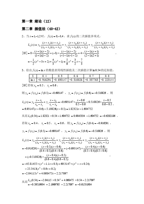
第一章 绪论(12) 第二章 插值法(40-42)2、当2,1,1-=x 时,4,3,0)(-=x f ,求)(x f 的二次插值多项式。
[解]372365)1(34)23(21)12)(12()1)(1(4)21)(11()2)(1()3()21)(11()2)(1(0))(())(())(())(())(())(()(2221202102210120120102102-+=-++--=+-+-⨯+------⨯-+-+-+⨯=----+----+----=x x x x x x x x x x x x x x x x x x x y x x x x x x x x y x x x x x x x x y x L 。
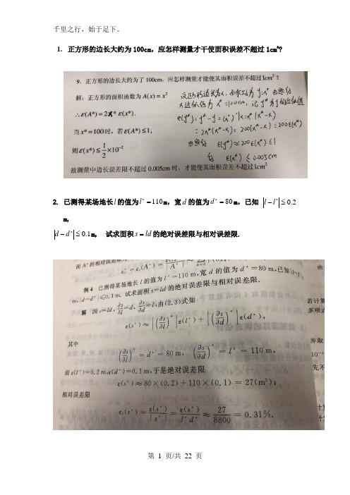
3、给出x x f ln )(=的数值表用线性插值及二次插值计算54.0ln 的近似值。
X 0.4 0.5 0.6 0.7 0.8 x ln -0.916291 -0.693147 -0.510826 -0.357765 -0.223144[解]若取5.00=x ,6.01=x ,则693147.0)5.0()(00-===f x f y ,510826.0)6.0()(11-===f x f y ,则604752.182321.1)5.0(10826.5)6.0(93147.65.06.05.0510826.06.05.06.0693147.0)(010110101-=---=--⨯---⨯-=--+--=x x x x x x x x x y x x x x y x L ,从而6202186.0604752.19845334.0604752.154.082321.1)54.0(1-=-=-⨯=L 。
若取4.00=x ,5.01=x ,6.02=x ,则916291.0)4.0()(00-===f x f y ,693147.0)5.0()(11-===f x f y ,510826.0)6.0()(22-===f x f y ,则 217097.2068475.404115.2)2.09.0(5413.25)24.0(3147.69)3.01.1(81455.45)5.06.0)(4.06.0()5.0)(4.0()510826.0()6.05.0)(4.05.0()6.0)(4.0()693147.0()6.04.0)(5.04.0()6.0)(5.0(916291.0))(())(())(())(())(())(()(22221202102210120120102102-+-=+--+-⨯++-⨯-=----⨯-+----⨯-+----⨯-=----+----+----=x x x x x x x x x x x x x x x x x x x x x x y x x x x x x x x y x x x x x x x x y x L ,从而61531984.0217097.21969765.259519934.0217097.254.0068475.454.004115.2)54.0(22-=-+-=-⨯+⨯-=L补充题:1、令00=x ,11=x ,写出x e x y -=)(的一次插值多项式)(1x L ,并估计插值余项。
数值分析题库答案(含详细解题步骤)
第 1 页/共 22 页1. 正方形的边长大约为100cm ,应怎样测量才干使面积误差不超过1cm 22. 已测得某场地长l 的值为110=*l m ,宽d 的值为80=*d m ,已知 2.0≤-*l l m,1.0≤-*d d m, 试求面积ld s =的绝对误差限与相对误差限.3.为使π的相对误差小于0.001%,至少应取几位有效数字?4.设x的相对误差界为δ,求n x的相对误差界.5.设有3个近似数a=2.31,b=1.93,c=2.24,它们都有3位有效数字,试计算p=a+bc的误差界和相对误差界,并问p的计算结果能有几位有效数字?第 3 页/共 22 页6. 已知333487.034.0sin ,314567.032.0sin ==,请用线性插值计算3367.0sin 的值,并预计截断误差.7. 已知sin0.32=0.314567, sin0.34=0.333487, sin0.36= 0.352274,用抛物插值计算sin0.3367的值, 并预计误差.8. 已知16243sin ,sin πππ===请用抛物插值求sin50的值,并预计误差9. . .6,8,7,4,1)(,5,4,3,2,1求四次牛顿插值多项式时设当==i i x f x第 5 页/共 22 页10. 已知4)2(,3)1(,0)1(=-=-=f f f , 求函数)(x f 过这3点的2次牛顿插 值多项式.11. 设x x f =)(,并已知483240.1)2.2(,449138.1)1.2(,414214.1)0.2(===f f f ,试用二次牛顿插值多项式计算(2.15)f 的近似值,并研究其误差12. 设],[)(b a x f 在上有四阶延续导数,试求满意条件)2,1,0()()(==i x f x P i i 及)()(11x f x P '='的插值多项式及其余项表达式.13. 给定3201219(),,1,,44f x x x x x ====试求()f x 在1944⎡⎤⎢⎥⎣⎦,上的三次埃尔米特插值多项式()P x ,使它满意11()()(0,1,2),()(),i i P x f x i P x f x ''===并写出余项第 7 页/共 22 页表达式.14. 设],1,0[,23)(2∈++=x x x x f 试求)(x f 在]1,0[上关于,,1{,1)(x span x =Φ=ρ}2x 的最佳平方逼近多项式15.已知实验数据如下:用最小二乘法求形如y=a+bx2的拟合曲线,并计算均方误差.16.已知数据表如下第 9 页/共 22 页x i 1 2 3 4 5 y iωi4 4.56 8 8.5 2 1 3 1 1试用最小二乘法求多项式曲线与此数据组拟合17. .1)(},1{span ,1]41[)(的最佳平方逼近多项式中的关于上的在在求==Φ=x x x x f ρ18. 决定求积公式⎰++≈10110)1()(32)0()(f A x f f A dx x f 中的待定参数110,,A x A , 使其代数精度尽量高,并指出所决定的求积公式的代数精度.19. 用复化辛普森公式计算积分⎰=10dx e I x , 问区间[0,1]应分多少等分才干使截断误差不超过?10215-⨯第 11 页/共 22 页20. 利用下表中给出的数据,分离用复化梯形公式和复化辛甫生公式计算定积分dx x I ln 21⎰=的近似值(要求结果保留到小数点后六位)21. 用复化梯形公式和复化辛甫生公式计算积分⎰=6.28.1)(dx x f I ,函数)(x f 在某些节点上的值如下图:(本题共14分)22. 决定公式⎰+≈101100)()()(x f A x f A dx x f x 的系数1010,,,x x A A ,使其具有最高代数精度23. 决定求积公式⎰++≈1110)1()(32)0()(f A x f f A dx x f 中的待定参数110,,A x A ,使其代数精度尽量高,并指出所决定的求积公式的代数精度第 13 页/共 22 页24.用LU 分解法求解以下方程组 (10分)123123142521831520x x x ⎛⎫⎛⎫⎛⎫ ⎪⎪ ⎪= ⎪⎪ ⎪ ⎪⎪ ⎪⎝⎭⎝⎭⎝⎭25.用LU 分解法求解以下方程组⎪⎪⎪⎭⎫ ⎝⎛=⎪⎪⎪⎭⎫ ⎝⎛⎪⎪⎪⎪⎪⎪⎭⎫ ⎝⎛8892121514131615141321x x x26. 用LU 分解法求解以下方程组⎪⎪⎪⎭⎫ ⎝⎛=⎪⎪⎪⎭⎫ ⎝⎛⎪⎪⎪⎭⎫⎝⎛542631531321321x x x27. 设方程组b Ax =,其中⎪⎪⎪⎭⎫⎝⎛-=220122101A ,Tb ⎪⎭⎫ ⎝⎛-=32,31,21, 已知它有解Tx ⎪⎭⎫⎝⎛-=0,31,21,若右端有小扰动61021-∞⨯=bδ,试预计由此引起的解的相对误差.第 15 页/共 22 页28. 设方程组b Ax =,其中212 1.0001A -⎛⎫= ⎪-⎝⎭,11.0001b -⎛⎫= ⎪⎝⎭,当右端向量b 有误差00.0001δ⎛⎫= ⎪⎝⎭b 时,试预计由此引起的解的相对误差(用∞范数计算)29. 给定b Ax =,其中⎥⎥⎥⎦⎤⎢⎢⎢⎣⎡=111a a a a a a A 证实:(1) 当121<<-a 时,A 对称正定,从而GS 法收敛. (2) 惟独当2121<<-a 时,J 法收敛.30. 对于线性方程组⎪⎩⎪⎨⎧-=+-=-+=+1242043 16343232121x x x x x x x ,列出求解此方程组的Jacobi 迭代格式,并判断是否收敛。
数值分析课后习题部分参考答案

数值分析课后习题部分参考答案Chapter 1(P10)5. 求2的近似值*x ,使其相对误差不超过%1.0。
解: 4.12=。
设*x 有n 位有效数字,则n x e -⨯⨯≤10105.0|)(|*。
从而,1105.0|)(|1*nr x e -⨯≤。
故,若%1.0105.01≤⨯-n,则满足要求。
解之得,4≥n 。
414.1*=x 。
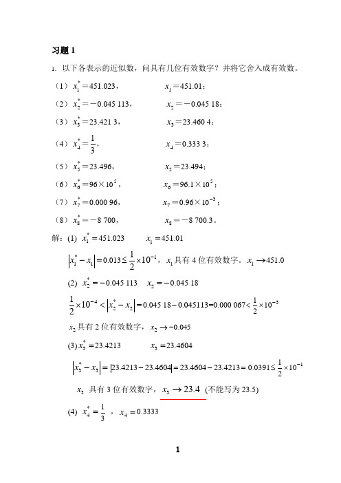
(P10)7. 正方形的边长约cm 100,问测量边长时误差应多大,才能保证面积的误差不超过12cm 。
解:设边长为a ,则cm a 100≈。
设测量边长时的绝对误差为e ,由误差在数值计算的传播,这时得到的面积的绝对误差有如下估计:e ⨯⨯≈1002。
按测量要求,1|1002|≤⨯⨯e 解得,2105.0||-⨯≤e 。
Chapter 2(P47)5. 用三角分解法求下列矩阵的逆矩阵:⎪⎪⎪⎭⎫ ⎝⎛--=011012111A 。
解:设()γβα=-1A。
分别求如下线性方程组:⎪⎪⎪⎭⎫ ⎝⎛=001αA ,⎪⎪⎪⎭⎫ ⎝⎛=010βA ,⎪⎪⎪⎭⎫ ⎝⎛=100γA 。
先求A 的LU 分解(利用分解的紧凑格式),⎪⎪⎪⎭⎫ ⎝⎛-----3)0(2)1(1)1(2)0(1)1(2)2(1)1(1)1(1)1(。
即,⎪⎪⎪⎭⎫ ⎝⎛=121012001L ,⎪⎪⎪⎭⎫⎝⎛---=300210111U 。
经直接三角分解法的回代程,分别求解方程组,⎪⎪⎪⎭⎫ ⎝⎛=001Ly 和y U =α,得,⎪⎪⎪⎭⎫ ⎝⎛-=100α;⎪⎪⎪⎭⎫ ⎝⎛=010Ly 和y U =β,得,⎪⎪⎪⎪⎪⎪⎭⎫⎝⎛=323131β;⎪⎪⎪⎭⎫ ⎝⎛=100Ly 和y U =γ,得,;⎪⎪⎪⎪⎪⎪⎭⎫ ⎝⎛--=313231γ。
所以,⎪⎪⎪⎪⎪⎪⎭⎫ ⎝⎛---=-3132132310313101A。
(P47)6. 分别用平方根法和改进平方根法求解方程组:⎪⎪⎪⎪⎪⎭⎫ ⎝⎛=⎪⎪⎪⎪⎪⎭⎫ ⎝⎛⎪⎪⎪⎪⎪⎭⎫ ⎝⎛----816211515311401505231214321x x x x 解:平方根法:先求系数矩阵A 的Cholesky 分解(利用分解的紧凑格式),⎪⎪⎪⎪⎪⎭⎫ ⎝⎛----1)15(2)1(1)5(3)3(3)14(2)0(1)1(1)5(2)2(1)1(,即,⎪⎪⎪⎪⎪⎭⎫⎝⎛--=121332100120001L ,其中,TL L A ⨯=。
《数值分析》所有参考答案
等价三角方程组
, ,
11.设计算机具有4位字长。分别用Gauss消去法和列主元Gauss消去法解下列方程组,并比较所得的结果。
解:Gauss消去法
回代
列主元Gauss消去
15.用列主元三角分解法求解方程组。其中
A= ,
解:
等价三角方程组
回代得
, , ,
16.已知 ,求 , , 。
解:
, ,
17.设 。证明
,(II)
,
当 时
当 时
迭代格式(II)对任意 均收敛
3) ,
构造迭代格式 (III)
,
当 时
当 时
迭代格式(III)对任意 均收敛
4)
取格式(III)
, , ,
4.用简单迭代格式求方程 的所有实根,精确至有3位有效数。
解:
当 时, ,
1 2
当 时
,
,
, ,
1)
迭代格式 ,
,
当 时, ,
任取 迭代格式收敛于
是中的一种向量范数。
解:
当 时存在 使得
,
,
所给 为 上的一个范数
18.设 。证明
(1) ;
(2) ;
(3) 。
解:(1)
(2)
(3)
19.设
A=
求 , , 及 , 。
解: ,
Newton迭代格式
,
20.设 为 上任意两种矩阵(算子)范数,证明存在常数
, 使得
对一切 均成立。
解:由向量范数的等价性知道存在正常数 使得
,
=0.187622
[23.015625 , 23.015625+0.187622]
数值分析期末复习题答案

数值分析期末复习题答案一、选择题1. 以下哪个算法是用于求解线性方程组的直接方法?A. 牛顿法B. 高斯消元法C. 共轭梯度法D. 辛普森积分法答案:B2. 插值法中,拉格朗日插值法和牛顿插值法的主要区别是什么?A. 插值点的选取不同B. 插值多项式的构造方式不同C. 计算复杂度不同D. 适用的函数类型不同答案:B3. 在数值积分中,梯形法则和辛普森法则的主要区别是什么?A. 精度不同B. 适用的积分区间不同C. 计算方法不同D. 稳定性不同答案:A二、简答题1. 解释什么是数值稳定性,并举例说明。
答案:数值稳定性指的是数值方法在计算过程中对于舍入误差的敏感程度。
例如,在求解线性方程组时,如果系数矩阵的条件数很大,则该方程组的数值解对舍入误差非常敏感,即数值稳定性差。
2. 说明数值微分与数值积分的区别。
答案:数值微分是估计函数在某一点的导数,而数值积分是估计函数在某个区间上的积分。
数值微分通常用于求解函数的局部变化率,而数值积分用于求解函数在一定区间内的累积效果。
三、计算题1. 给定一组数据点:(1, 2), (2, 3), (3, 5), (4, 6),请使用拉格朗日插值法构造一个三次插值多项式。
答案:首先写出拉格朗日插值基函数,然后根据数据点构造插值多项式。
具体计算过程略。
2. 给定函数 f(x) = x^2,使用牛顿-科特斯公式中的辛普森积分法在区间 [0, 1] 上估计积分值。
答案:首先确定区间划分,然后应用辛普森积分公式进行计算。
具体计算过程略。
四、论述题1. 论述数值分析中误差的来源及其控制方法。
答案:误差主要来源于舍入误差和截断误差。
舍入误差是由于计算机在进行浮点数运算时的精度限制造成的,而截断误差是由于数值方法的近似性质导致的。
控制误差的方法包括使用高精度的数据类型、选择合适的数值方法、增加计算步骤等。
五、综合应用题1. 给定一个线性方程组 Ax = b,其中 A 是一个 3x3 的矩阵,b 是一个列向量。
数值分析课后部分习题答案
解
x * = 2.00021 = 0.200021 × 101 ,即 m = 1
1 1 × 10m − n = × 10−3 , 2 2
由有效数字与绝对误差的关系得 即
m − n = −3 ,所以, n = 2 ; y* = 0.032 = 0.32 × 101 ,即 m = 1
由有效数字与绝对误差的关系得 即
m − n = −3 ,所以, n = 4 ; z * = 0.00052 = 0.52 × 10⁻³ ,即 m = −3
1 1 × 10m − n = × 10−3 , 2 2
由有效数字与绝对误差的关系得 即
m − n = −3 ,所以, n = 0 .
1 1 × 10m − n = × 10−3 ,Fra bibliotek2 2=
f [x1 , x2 ,⋯ , x n ]-f [ x0 , x1 ,⋯ , x n−1 ] g[ x1 , x2 ,⋯ , x n ] − g[ x0 , x1 ,⋯ , x n−1 ] + x n − x0 x n − x0
( x − 1)( x − 2)( x − 3) 1 =- ( x − 1)( x − 2)( x − 3) , (0 − 1)(0 − 2)(0 − 3) 6
x ( x − 2)( x − 3) 1 = x ( x − 2)( x − 3) , (1 − 0)(1 − 2)(1 − 3) 2 x( x − 1)( x − 3) 1 =- x( x − 1)( x − 3) , (2 − 0)(2 − 1)(2 − 3) 2 x( x − 1)( x − 2) 1 = x ( x − 1)( x − 2) , (3 − 0)(3 − 1)(3 − 2) 6
数值分析课程课后习题答案(李庆扬等)1
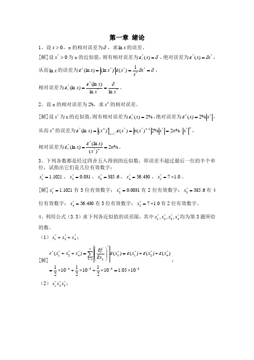
第一章 绪论1、设0>x ,x 的相对误差为δ,求x ln 的误差。
[解]设0*>x 为x 的近似值,则有相对误差为δε=)(*x r ,绝对误差为**)(x x δε=,从而x ln 的误差为δδεε=='=*****1)()(ln )(ln x x x x x , 相对误差为****ln ln )(ln )(ln x x x x rδεε==。
2、设x 的相对误差为2%,求n x 的相对误差。
[解]设*x 为x 的近似值,则有相对误差为%2)(*=x r ε,绝对误差为**%2)(x x =ε,从而n x 的误差为nn x x nxn x x n x x x **1***%2%2)()()()(ln *⋅=='=-=εε,相对误差为%2)()(ln )(ln ***n x x x nr==εε。
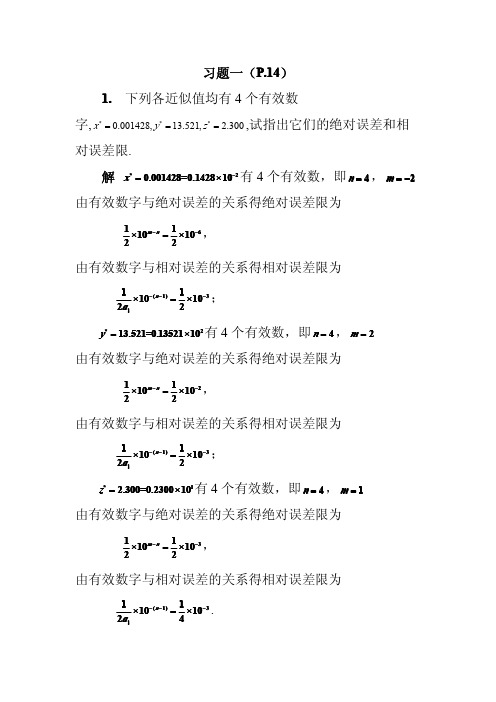
3、下列各数都是经过四舍五入得到的近似数,即误差不超过最后一位的半个单位,试指出它们是几位有效数字:1021.1*1=x ,031.0*2=x ,6.385*3=x ,430.56*4=x ,0.17*5⨯=x 。
[解]1021.1*1=x 有5位有效数字;0031.0*2=x 有2位有效数字;6.385*3=x 有4位有效数字;430.56*4=x 有5位有效数字;0.17*5⨯=x 有2位有效数字。
4、利用公式(3.3)求下列各近似值的误差限,其中*4*3*2*1,,,x x x x 均为第3题所给的数。
(1)*4*2*1x x x ++; [解]3334*4*2*11***4*2*1*1005.1102110211021)()()()()(----=⨯=⨯+⨯+⨯=++=⎪⎪⎭⎫ ⎝⎛∂∂=++∑x x x x x f x x x e nk k k εεεε;(2)*3*2*1x x x ;[解]52130996425.010********.2131001708255.01048488.2121059768.01021)031.01021.1(1021)6.3851021.1(1021)6.385031.0()()()()()()()()(3333334*3*2*1*2*3*1*1*3*21***3*2*1*=⨯=⨯+⨯+⨯=⨯⨯+⨯⨯+⨯⨯=++=⎪⎪⎭⎫⎝⎛∂∂=-------=∑x x x x x x x x x x x f x x x e n k k kεεεε;(3)*4*2/x x 。
数值分析课后习题答案

7、计算的近似值,取。
利用以下四种计算格式,试问哪一种算法误差最小。
〔1〕〔2〕〔3〕〔4〕解:计算各项的条件数由计算知,第一种算法误差最小。
解:在计算机上计算该级数的是一个收敛的级数。
因为随着的增大,会出现大数吃小数的现象。
9、通过分析浮点数集合F=〔10,3,-2,2〕在数轴上的分布讨论一般浮点数集的分布情况。
10、试导出计算积分的递推计算公式,用此递推公式计算积分的近似值并分析计算误差,计算取三位有效数字。
解:此算法是数值稳定的。
第二章习题解答1.〔1〕 R n×n中的子集“上三角阵〞和“正交矩阵〞对矩阵乘法是封闭的。
〔2〕R n×n中的子集“正交矩阵〞,“非奇异的对称阵〞和“单位上〔下〕三角阵〞对矩阵求逆是封闭的。
设A是n×n的正交矩阵。
证明A-1也是n×n的正交矩阵。
证明:〔2〕A是n×n的正交矩阵∴A A-1 =A-1A=E 故〔A-1〕-1=A∴A-1〔A-1〕-1=〔A-1〕-1A-1 =E 故A-1也是n×n的正交矩阵。
设A是非奇异的对称阵,证A-1也是非奇异的对称阵。
A非奇异∴A可逆且A-1非奇异又A T=A ∴〔A-1〕T=〔A T〕-1=A-1故A-1也是非奇异的对称阵设A是单位上〔下〕三角阵。
证A-1也是单位上〔下〕三角阵。
证明:A是单位上三角阵,故|A|=1,∴A可逆,即A-1存在,记为〔b ij〕n×n由A A-1 =E,那么〔其中 j>i时,〕故b nn=1, b ni=0 (n≠j)类似可得,b ii=1 (j=1…n) b jk=0 (k>j)即A-1是单位上三角阵综上所述可得。
R n×n中的子集“正交矩阵〞,“非奇异的对称阵〞和“单位上〔下〕三角阵〞对矩阵求逆是封闭的。
2、试求齐次线行方程组Ax=0的根底解系。
A=解:A=~~~故齐次线行方程组Ax=0的根底解系为,3.求以下矩阵的特征值和特征向量。
- 1、下载文档前请自行甄别文档内容的完整性,平台不提供额外的编辑、内容补充、找答案等附加服务。
- 2、"仅部分预览"的文档,不可在线预览部分如存在完整性等问题,可反馈申请退款(可完整预览的文档不适用该条件!)。
- 3、如文档侵犯您的权益,请联系客服反馈,我们会尽快为您处理(人工客服工作时间:9:00-18:30)。
Answers for Exercises —Numerical methods using MatlabChapter 1P10 2. Solution (a) )(x g x = produces an equation 0862=+-x x . Solving it gives the roots 2=x and 4=x .Since 2)2(=g and 4)4(=g , thus, both 2=P and 4=P are fixed points of )(x g . (b) –(d) The iterative rule using )(x g is 22144n n n p p p ---=. The results for part (b)-(d) with starting value 9.10=p and 8.30=p are listed in Table 1.(e) Calculate values of x x g -='4)( at 2=x and 4=x .12)2(>='g , and 10)4(<='g .Since )(x g ' is continuous, there exists a number 0>δ such that1)(<'x g for all ]4,4[δ+δ-∈x .There also exists a number 0>λ such that1)(>'x g for all ]2,2[λ+λ-∈x .Therefore, for 4=p , all hypotheses of Theorem 1.3 are satisfied. The sequencegenerated by 22144n n n p p p ---=with starting value 8.30=p converges to 4=p . But it doesn ’t true for 2=p with starting value 9.10=p .P11 4. Find the fixed point for )(x g : )(x g x = gives 2±=p . Find the derivative: 12)(+='x x g .Evaluate )2(-'g and )2(g ': 3)2(-=-'g , 5)2(='g .Both 2-=p and 2=p give 1)(>'p g . There is no reason to find the solution(s)using the fixed-point iteration.P11 6. Proof ))(()()(010112p p g p g p g p p -ξ'=-=-)()()( 0101p p K p p g -<-ξ'≤P21 4 For false position method, the approximation of the root at each step is)()())((n n n n n n n a f b f a b b f b c ---=,where ],[n n b a contains the root.The results using false position method are listed in theTable 210. (a) The results using Bisection method are listed in Table 3.The values of tant(x) at midpoints are going to zero while the sequence convergeszero unless the midpoints are very close to the root, say, in [1.4, pi/2).P36 2& 9. The first derivative of 3)(2--=x x x f is 12)(-='x x f . The Newton-Raphson formula is 12321-+=+n n n p p p . The results are listed in Table 5.The sequence generated by 12321-+=+n n n p p p with the starting value p 0=0.0 disverges. The Secant iterative rule is )3()3())(3(1212121---------=---+n n n n n n n n n n p p p pp p p p p pResults are listed in Table 6 with p 0=1.7 and p 1 =1.67.·Answers for Exercises —Numerical methods using MatlabChapter 2P44 2. Solution The 4th equation yields 24=x .Substituting 24=x to the 3rd equation gives 53=x .Substituting both 24=x and 53=x to the 2nd equation produces 32-=x . 21=x is obtained by sustituting all 32-=x , 53=x and 24=x to the 1st equation. The value of the determinant of the coefficient matrix is 115573115=⨯⨯⨯=D .4. Proof (a) Calculating the product of the two given upper-triangular matrices gives⎥⎥⎥⎦⎤⎢⎢⎢⎣⎡++++=⎥⎥⎥⎦⎤⎢⎢⎢⎣⎡⎥⎥⎥⎦⎤⎢⎢⎢⎣⎡=33333323232222223313231213112212121111113323221312113323221312110000b a b a b a b a b a b a b a b a b a b a b b b b b b a a a a a a B A . It is also an upper-triangular matrix.(b) Let N N ij a A ⨯=)( and N N ij b B ⨯=)( where 0=ij a and 0=ij b when j i >.Let N N ij c B A C ⨯==)(. According to the definition of product of the two matrices, we have∑==Nk kjik ij b ac 1for all N j i ,,2,1, =.0=ij c when j i > because 0=ij a and 0=ij b when j i >.That means that the product of the two upper-triangular matrices is also upper triangular.5. Solution From the first equation we have 31=x .Substituting 31=x to the second equation gives 22=x .13=x is obtained from the third equation and 14-=x is attained from the last equation.The value of the determinant of the coefficient is 243)1(42)det(-=⨯-⨯⨯=A7. Proof The formula of the back substitution for an N N ⨯upper-triangular system is NNN a b x =and kkNk j jkj k k a x a b x ∑+=-=1 for 1,,2,1 --=N N k .The process requiresN N=+++111 divisions, 22)1()1(212NN N N N -=-=-+++ multiplications, and2)1(212NN N -=-+++ additions or subtractions.P53 1. Solution Using elementary transformations for the augment matrix gives330012630464275101263046425232103514642],[3231213121⎥⎥⎥⎦⎤⎢⎢⎢⎣⎡--−−→−⎥⎥⎥⎦⎤⎢⎢⎢⎣⎡---−−−→−⎥⎥⎥⎦⎤⎢⎢⎢⎣⎡--=++-+-r r r r r r B ASo the system ⎪⎩⎪⎨⎧=++=++-=-+523 1035 4642321321321x x x x x x x x x is equivalent to the upper-triangular system⎪⎩⎪⎨⎧==+-=-+33 1263 4642332321x x x x x x 11. Solution Using the algorithm of Gaussian Elimination gives12420010324050110700211242001032409013270021],[212⎥⎥⎥⎥⎦⎤⎢⎢⎢⎢⎣⎡----−−−→−⎥⎥⎥⎥⎦⎤⎢⎢⎢⎢⎣⎡--=+-r r B A ⎥⎥⎥⎥⎦⎤⎢⎢⎢⎢⎣⎡------−−→−+1242001032005011070021324r r ⎥⎥⎥⎥⎦⎤⎢⎢⎢⎢⎣⎡------−−→−+21000103200501107002143r r The set of solutions of the system is obtained by the back substitutions,3,2,2234==-=x x x and .11=x14. (a) (i) Solution Applying Gaussian elimination with partial pivoting to the augment matrix results in⎥⎥⎥⎦⎤⎢⎢⎢⎣⎡---−−→−⎥⎥⎥⎦⎤⎢⎢⎢⎣⎡---=↔1100320001.0101001.01003001.010030001.010*******],[31r r B A⎥⎥⎥⎦⎤⎢⎢⎢⎣⎡--−−→−⎥⎥⎥⎦⎤⎢⎢⎢⎣⎡--−−→−↔+-+-00043.03333.43019933.996667.630001.0100319933.996667.63000043.03333.430001.01003 3231213231r r r r r r ⎥⎥⎥⎦⎤⎢⎢⎢⎣⎡---−−−−→−+-6806.00625.680019933.996667.630001.01003326667.633333.43r rThe set of solutions is,101.0524,0100.0-623⨯==x x and .105.2400 -61⨯=x15. Solution The N N ⨯Hilbert matrix is defined byN N ij H H ⨯=)( where 11-+=j i H ij for N j i ≤≤,1.(a) The inverse of the 44⨯ Hilbert matrix is⎥⎥⎥⎥⎦⎤⎢⎢⎢⎢⎣⎡--------=-280042001680140420064802700240168027001200120140240120161H The exact solution is T X )140,240,120,16(--=.(b) The solution is T X )0881.185,0628.310,6053.149,7308.18(--=. A miss is as good as a mile. (失之毫厘,谬以千里)P62 5 (a) Solving B LY = gives TY )2,12,6,8(-=.From Y UX = we have TX )2,1,1,3(-=. The product of A and X is TAX )4,10,4,8(--=. That means B AX =(b) Similarly to the part (a), we haveTY )1,12,6,28(=, TX )1,2,1,3(=, and B AX T==)4,23,13,28(.6.⎥⎥⎥⎥⎦⎤⎢⎢⎢⎢⎣⎡---=175.113011*********L , ⎥⎥⎥⎥⎦⎤⎢⎢⎢⎢⎣⎡-----=5.70001040085304011UP72 7. (a) Jacobi Iterative formula is()⎪⎪⎩⎪⎪⎨⎧-+=+-=++-=+++)()()1()()()1()()()1(226141358k k k k k k k k k y x z z x y z y x for ,2,1,0=kResults for ),,()()()(k k k k z y xP =, ,3,2,1=k are listed in Table 2.1 with starting value )0,0,0(0=P .Jacobi iteration does not converge(b) Gauss-Seidel Iterative formula is()⎪⎪⎩⎪⎪⎨⎧-+=+-=++-=++++++)1()1()1()()1()1()()()1(226141358k k k k k k k k k y x z z x y z y x for ,2,1,0=kResults ),,()()()(k k k k z y xP =, ,3,2,1=k are listed in Table 2.2 with starting value )0,0,0(0=PGauss-Seidel iteration does not converge as well.Reasons:Conside the eigenvalues of iterative matricesSplit the coefficient matrix ⎥⎥⎥⎦⎤⎢⎢⎢⎣⎡----=612114151A into three matrices⎥⎥⎥⎦⎤⎢⎢⎢⎣⎡-⎥⎥⎥⎦⎤⎢⎢⎢⎣⎡---⎥⎥⎥⎦⎤⎢⎢⎢⎣⎡-=--=000100150012004000600010001U L D A .The iterative matrix of Jacobi iteration is⎥⎥⎥⎥⎦⎤⎢⎢⎢⎢⎣⎡--=⎥⎥⎥⎦⎤⎢⎢⎢⎣⎡----⎥⎥⎥⎥⎦⎤⎢⎢⎢⎢⎣⎡=+=-061311041500121041506100010001)(1U L D T JThe spectral raduis of J T is 16800.5)(>=ρJ T . )1176.0,4546405880(i . .-±=λ So Jacobi method doesnot converge.Similarly, the iterative matrix of Gauss-Seidel iteration is⎥⎥⎥⎥⎦⎤⎢⎢⎢⎢⎣⎡--=-=-65503200150)(1U L D T G .The spectral radius of G T is 2532.19)(=ρG T >1. )0866.0,2532.19,0(-=λ So Gauss-Seidel method does not converge.8. (a) Jacobi Iterative formula is()⎪⎩⎪⎨⎧-+=-+=+-=+++6/225/)8(4/)13()()()1()()()1()()()1(k k k k k k k k k y x zz x y z y x for ,2,1,0=k ),,()()()(k k k k z y x P = for 10,,2,1 =k are listed in Table 2.3 with starting value )0,0,0(0=P .Table 2.30 0 0 3.2500 1.6000 0.3333 2.9333 2.1833 1.1500 2.9917 1.9567 0.9472 2.9976 2.0089 1.0044 2.9989 1.9986 0.99772.9998 2.0002 0.9999 2.9999 2.0000 0.99993.0000 2.0000 1.0000 3.0000 2.0000 1.0000Jacobi iteration converges to the solution (3, 2, 1)(b) Gauss-Seidel iterative formula is()⎪⎪⎩⎪⎪⎨⎧+---=+---=+-=++++++)1()1()1()()1()1()()()1(22615/)8(4/)13(k k k k k k k k k y x z z x y z y x for ,2,1,0=k ),,()()()(k k k k z y x P = for 10,,2,1 =k are listed in Table 2.4 with starting value )0,0,0(0=PTable 2.40 0 0 3.2500 2.2500 1.0417 2.9479 1.9813 0.9858 3.0011 2.0031 0.9999 2.9992 1.9999 0.9998 3.0000 2.0000 1.0000 3.0000 2.0000 1.0000 3.0000 2.0000 1.0000 3.0000 2.0000 1.0000 3.0000 2.0000 1.0000Gauss-Seidel iteration converges to the solution (3, 2, 1)Answers for Exercises —Numerical methods using MatlabChapter 3P99 1. Solution (a) The nth order derivative of )sin()(x x f = is )2sin()()(π+=n x x f n .Therefore, !5!3)(535x x x x P +-=, !7!5!3)(7537x x x x x P -+-= and !9!7!5!3)(97539x x x x x x P +-+-=.(b) Estimating the remainder term gives71091075574.2!101!10)5sin()(-⨯≤≤π+=x c x E for 1≤x .(c) Substituting 4π=x to )2sin()()(π+=n x x f n gives ,22)4()4(,22)4()4()3(-=π=π''=π'=πf f f f and 22)4()4()5()4(-=π=πf f .By using Taylor polynomial we have!5)4(22!4)4(22!3)4(22!2)4(22)4(2222)(54325π-+π-+π--π--π-+=x x x x x x P P108 1. (a) Using th e Horner ’s method to find )4(P givesSo )4(P =1.18.(b) From part (a) we have 12.002.002.0)(2-+-=x x x Q . )4()4(Q P =' can be also obtained byusing Horner ’s method.So )4(P '=-0.36 Another method:Hence, P(4)=-0.36.(c) Find )4(I and )1(I firstly.Then=-=⎰)1()4()(41I I dx x P 4.3029.(d) Use Horner ’s method to evaluate P (5.5)Hence, P (5.5)=0.2575.(e) Let 012233)(a x a x a x a x P +++=. There are 4 coefficients need to be found. Substituting four known point ),(i i y x , i =1, 2, 3, 4, to )(x P gives four linear equations with unknown i a , i =1, 2, 3, 4. The coefficients can be found by solving this linear system.P120 1. The values of f (x ) at the given points are listed in Table 3.1:(a) Find the Lagrange coefficient polynomials and 010)(0,1x x x L -=---=.1101)(1,1+=++=x x x LThe interpolating polynomial is x x L f x L f x P =+-=)()0()()1()(1,10,11. (b) ),(21)11()1()(20,2x x x x x L -=----=,110)1)(1()(21,2x x x x L -=--+=),(212)1()(22,2x x x x x L +=+=x x L f x L f x L f x P =++-=)()1()()0()()1()(2,21,20,22. (c) ),2)(1(61)21)(11()2)(1()(0,3---=-------=x x x x x x x L),2)(1)(1(21)20)(10)(10()2)(1)(1()(1,3--+=--+--+=x x x x x x x L),2)(1(21)21(1)11()2()1()(2,3-+-=-+-+=x x x x x x x L),1)(1(61)12(2)12()1()1()(3,3-+=-+-+=x x x x x x x L33,32,31,30,33)()2()()1()()0()()1()(x x L f x L f x L f x L f x P =+++-=(d) ,2212)(0,1x x x L -=--=,1121)(0,1-=--=x x x L67)()2()()1()(1,10,11-=+=x x L f x L f x P . (e) ),23(21)20)(10()2)(1()(20,2+-=----=x x x x x L ),2()21(1)2()(21,2x x x x x L --=--=),(21)12(2)1()(20,2x x x x x L -=--=.23)()2()()1()()0()(22,21,20,22x x x L f x L f x L f x P -=++=7. (a) Note that each Lagrange polynomial )(,2x L k is of degree at most 2 and )(x g is a combination of)(,2x L k . Hence )(x g is also a polynomial of degree at most 2.(b) For each k x , 2,1,0=k , the Lagrange coefficient polynomial 1)(,2=k k x L , and 0)(,2=k j x L for k j ≠, 2,1,0=j . Therefore, 01)()()()(2,21,20,2=-++=k k k k x L x L x L x g .(c) )(x g is a polynomial of degree 2≤n and has n ≥ 3 zeroes. According to the fundamental theorem of algebra, 0)(=x g for all x .9. Let )()()(x P x f x E N N -=. )(x E N is a polynomial of degree N ≤.)(x f is degree with )(x P N at N +1 points N x x x ,,,10 implies that )(x E N has N +1 zeroes. Therefore, 0)(=x E N for all x , that is, )()(x P x f N = for all x .P131 6. (a) Find the divided-difference table:(b) Find the Newton polynomials with order 1, 2, 3 and 4.)0.1(80.16.3)(1--=x x P , )0.2)(0.1(6.0)0.1(80.160.3)(2--+--=x x x x P , )0.3)(0.2)(0.1(15.0)0.2)(0.1(6.0)0.1(80.16.3)(3------+--=x x x x x x x P ,)0.4)(0.3)(0.2)(0.1(03.0 )0.3)(0.2)(0.1(15.0)0.2)(0.1(6.0)0.1(80.16.3)(4----+------+--=x x x x x x x x x x x P .(c)–(d) The results are listed in Table 3.2P143 6. x x x T 32)(323-=, ]1,1[-∈x .The derivative of )(3x T is 323)(223-⋅='x x T . 0)(3='x T yields 21±=x . Evaluating )(3x T at 21±=x and 1±=x gives 1)1(3-=-T , 1)21(3=-T , 1)21(3-=T and 1)1(3=T .Therefore, 1))(max(3=x T , 1))(min(3-=x T . 10. When 2=N , the Chebyshev nodes are ,23)6/5cos(0-=π=x ,01=xand 23)6/cos(2=π=x .Calculating the Lagrange coefficient polynomials based on 210,,x x x can be obtained the results.Answers for Exercises —Numerical methods using MatlabChapter 4P157 1(a). Solution The sums for obtaining Normal equations are listed in Table 4.1The normal equation is ,710=A 135=B . Then ,7.0=A 6.2=B .The linear-squares line is 6.27.0+=x y .2449.0)((51)(215122=⎪⎪⎭⎫ ⎝⎛-=∑=k k k x f y f EP158 4. Proof Suppose the linear-squares line is B Ax y += where A and B are satisfiedthe Normal equations ∑∑===+N k k Nk ky xAB N 11and ∑∑∑====+Nk k k N k k N k k y x x A x B 1121.y yN x A B N N B x NA B x A Nk kNk k Nk k ==⎪⎪⎭⎫ ⎝⎛+=+⎪⎪⎭⎫ ⎝⎛=+∑∑∑===111111meas thatthe point ),(y x lies on the linear-squares line B Ax y +=.5. First eliminating B on the Normal equations∑∑===+Nk k Nk k y x A B N 11and ∑∑∑====+Nk k k Nk k Nk k y x x A x B 1121gives⎪⎪⎭⎫ ⎝⎛-=∑∑∑===Nk k N k k N k k k y x y x N D A 1111 where 2112⎪⎪⎭⎫ ⎝⎛-=∑∑==N k k N k k x x N D . Substituting A into the first equation gets⎪⎪⎭⎫⎝⎛⎪⎪⎭⎫ ⎝⎛+-=∑∑∑∑∑=====Nk k Nk k Nk k k N k k N k k y x N y x x y N D D B 12111111. Note that ∑∑∑∑∑∑∑∑========⎪⎪⎭⎫ ⎝⎛-=⎪⎪⎭⎫ ⎝⎛⎪⎪⎭⎫ ⎝⎛-=N k k N k k N k k N k k N k k N k k Nk k N k k y x N y x y x x N N y N D 12111212112111. Simplifying B gives⎪⎪⎭⎫ ⎝⎛-=∑∑∑∑====Nk k k N k k Nk k N k k y x x y x D B 111121.8(b). The sums needed in the Normal equations are listed in Table 4.26177.142==∑∑kkkxy x A )2(=M5606.063==∑∑kkkx y xB )3(=MHence, 26177.1x y = and 35606.0x y =.0.3594 )(51)(21512222=⎪⎪⎭⎫⎝⎛-=∑=k k k Ax y Ax E , 1.1649 )(51)(21512332=⎪⎪⎭⎫⎝⎛-=∑=k k k Bx y Bx E .26175.1x y = fits the given data better.P171 2(c). The sums for normal equations are listed in Table 4.3.Using the formulaproduces the system with unkowns A , B , and CSolving the obove system gives .6.0,1.0,5.2-=-==C B A The fitting curve is .6.01.05.22--=x x y∑∑∑∑∑∑∑∑∑∑∑============++=++=++512514513512515135125151512515k kk k k k k k k k kk k k k k k k k k k k k k y x x A x B x C y x x A x B x C y x A x B C .793410,110,22105=+-==+A C B A CP172 4. (a) Translate points in x-y plane into X-Y plane using y Y x X ln ,==. The results arelisted in Table 4.4.The Normal equationsgive the system Then -0.50844=A , 1.3524=B . Thus 866731.3524.e e C B ===.The fitting curve is xe.y 50844.086673-=, and 1190.0)((51)(215122=⎪⎪⎭⎫ ⎝⎛-=∑=k k k x f y f E .(b) Translate points in x-y plane into X-Y plane using yY x X 1,==. The results are listed in Table 4.5.∑∑∑∑∑======+=+515125151515k kk k k k k k kk k Y X X A X B Y X A B .8648.0155,2196.455-=+=+A B A BThe Normal equationsgive the system Then 2432.0=A , 30280.0=B .The fitting curve is 30280.02432.01+=x y and 5548.4)((51)(215122=⎪⎪⎭⎫ ⎝⎛-=∑=k k k x f y f E .(c) It is easy to see that the exponential function is better comparing with errors in part (a) and part (b).P188 1. (a) Derivativing )(x S gives 232132)(x a x a a x S ++='. Substituting the conditionspruduces the system of equations. ⎪⎪⎩⎪⎪⎨⎧=++=+++=++=+++0124 2842032 132132103213210a a a a a a a a a a a a a a(b) Solving the linear system of equations in (a) gives 29,,12,63210-==-==a a a a . The cubic polynomial is 3229126)(x x x x S -+-=..1620.5155,7300.255=+=+A B A B ∑∑∑∑∑======+=+515125151515k k k k k k k k kk k Y X X A X B Y X A BFigure: Graph of the cubic polynomial4. Step 1 Find the quantities: 3,1210===h h h , 21/)20(/)(0010-=-=-=h y y d13/)03(/)(1121=-=-=h y y d , 6667.03/)31(/)(2232-=-=-=h y y d 18)(6011=-=d d u , 10)(6122-=-=d d uStep 2 Use ⎪⎪⎩⎪⎪⎨⎧-'-=⎪⎭⎫ ⎝⎛++'--=+⎪⎭⎫⎝⎛+))((3232))((32232322211100121110d x S u m h h m h x S d u m h m h h to obtain the linear system⎩⎨⎧-=+=+0001.155.1032135.72121m m m m .The solutions are 5161.2,8065.321-==m m .Step 3 Compute 0m and 3m using clamaped boundary. 4.90322))((310000-=-'-=m x S d h m , 2.9248 2))((322323=--'=md x S h m Step 4 Find the spline coefficients16)2(,210001,000,0-=+-===m m h d s y s , 1.45166,-2.451620013,002,0=-===h m m s m s ;-1.54856)2(,021111,110,1=+-===m m h d s y s , -0.35136,1.903321123,112,1=-===h m m s m s ;0.38716)2(,332221,220,2=+-===m m h d s y s , 0.30236,-1.258122233,222,2=-===h m m s m s ; Therefore, 320)3(4516.1)3(4516.2)3(2)()(+++-+-==x x x x S x S for 23-≤≤-x , 321)2(3513.0)2(903.1)2(5484.1)()(+-+++-==x x x x S x S for 12≤≤-x , and322)1(3023.0)1(2581.1)1(3871.03)()(-+---+==x x x x S x S for 41≤≤x .5. Calculate the quantities: 3,1210===h h h , 20-=d ,11=d , 6667.02-=d ,181=u , 102-=u . ( Same values as Ex. 4)Substituting }{j h , }{j d and }{j u into ()()⎩⎨⎧=++=++22211112111022u m h h m h u m h m h h gives ⎩⎨⎧-=+=+1012318382121m m m mSolve the linear equation to obtain .5402.1,8276.221-==m m In addition, .030==m m Find the spline coefficients:4713.26)2(,210001,000,0-=+-===m m h d s y s , 4713.06,020013,002,0=-===h m m s m s ; -1.05756)2(,021111,110,1=+-===m m h d s y s , -0.24276,4138.121123,112,1=-===h m m s m s ;8735.06)2(,332221,220,2=+-===m m h d s y s , 0856.06,7701.0-22233,222,2=-===h m m s m s . Therefore, 30)3(4713.0)3(4713.22)(-++-=x x x S , for 23-≤≤-x ;321)2(2427.0)2(4138.1)2(0575.1)(+-+++-=x x x x S , for 12≤≤-x322)1(0856.0)1(7701.0)1(8735.03)(-+---+=x x x x S for 41≤≤x .Answers for Exercises —Numerical methods using MatlabChapter 5P209 1(b). Solution LetThe result of using the trapezoidal rule with h =1 isUsing Simpson’s rule with h=1/2, we haveFor Simpson’s 3/8 rule with h=1/3, we obtainThe result of using the Boole’s rule with h=1/4 is4. Proof Integrate )(1x P over ],[10x x .11102012101)(2)(2)(x x x x x x x x hfx x hf dx x P -+--=⎰=)(210f f h+. The Quadrature formula )(2)(101f f hdx x f x x +≈⎰is called the trapezoidal rule.6. Solution The Simpson ’s rule is)4(3)(2101f f f hdx x f x x ++≈⎰. It will suffice to apply Simpson ’s rule over the interval [0, 2] with the test functions32,,,1)(x x x x f = and 4,x . For the first four functions, since).4cos(1)(x e x f x -+=..f f f f h dx x f 3797691))1()0((21)(2)(1010=+=+≈⎰.9583190))1()5.0(4)0((61)4(3)(21010. f f f f f f h dx x f =++=++≈⎰.9869270 ))1()3/2(3)3/1(3)0(( 8/1 )33(83)(321010.f f f f f f f f hdx x f =+++=+++≈⎰.008761 ))1(7)4/3(32)2/1(12)4/1(32)0(7( 90/1 )73212327(452)(432101.f f f f f f f f f f hdx x f =++++=++++≈⎰)1141(31212+⨯+==⎰dx , )2140(31220+⨯+==⎰xdx , )4140(3138202+⨯+==⎰dx x , )8140(314203+⨯+==⎰dx x , the Simpson ’s rule is exact. But for 4)(x x f =,)16140(3153224+⨯+≠=⎰dx x . .Therefore, the degree of precision of Simpson ’s rule is n =3.T he Simpson’s rule and the Simpson ’s 3/8 rule have the same degree of precision n =3.P220 3(a) Solution When 3)(x x f =for 10≤≤x , ⎰+π=123912dx x x area .The values of 2391)(x xx g +=at 11 sample points (M =10) are listed in the Table 5.1:Table 5.1(i) Using the composite Trapezoidal rule ∑-=++=110)()()((2),(M k k M x g h x g x g hh g T , the computation is)9156.11084.16098.03719.01563.00710.00280.00081.00010.0(101)1623.30(201)101,(++++++++++=g T=)2160.4(101)1623.3(201+=0.1576+0.4216=0.5792.(ii) Using the composite Simposon ’s rule ∑∑-=--=+++=11121120)(34)(32)()((3),(M k k M k k M x g h x g h x g x g h h g S , the computation is)9156.16098.01563.00280.00010.0(304)1084.13719.00710.00081.0(302 )1623.30(301)101,(++++++++++=g S=)7106.2(304)5054.1(302 )1623.3(301++=0.5672.7. (a) Because the formula)2()1()0()(2102g w g w g w dt t g ++=⎰is exact for the three functions 1)(=t g ,x t g =)(, and 2)(x t g =, we obtain three equations with unkowns 0w , 1w , and 2w :2210=++w w w ,2221=+w w ,38421=+w w . Solving this linear system gives 310=w , 341=w and 312=w .Thus, ())2()1(4)0(31)(20g g g dt t g ++=⎰(b) Let ht x x +=0 and denote ,01h x x +=.202h x x +=Then the change of variable ht x x +=0 translates ],[20x x into [0, 2] and converts the integral expresion dx x f )( into dt ht x hf )(0+. Hence,()())()(4)(3)2()1(4)0(3)()()(21022002x f x f x f h g g g hdt t g h dt ht x f h dx x f x x ++=++==+=⎰⎰⎰. The formula ())()(4)(3)(21020x f x f x f hdx x f x x ++=⎰ is known as the Simpson ’s rule over ],[20x x .8(a).9(a).P234 1(a) Let 212sin )(x xx f +=. The Romberg table with three rows for ⎰+3212sin dx x xis given as follows:].6/,6/[],[ and cos )(Let ππ-==b a x x f hav e we , and cos )( ,sin )( Since Mab h x x f x x f -=-=''-='.10513/123/ )(12),(922-⨯<⨯⎪⎭⎫ ⎝⎛ππ≤''--=M c f h a b h f E T .1039.2/)( and )4375( 9.4374 So,4-⨯≈-==>M a b h M M ].6/,6/[],[ and cos )(Let ππ-==b a x x f ,cos )( ,sin )( , cos )( ,sin )( Since )4(x x f x x f x x f x x f =='''-=''-='.105123/1803/ )(180),(92)4(4-⨯<⨯⎪⎭⎫ ⎝⎛ππ≤--=M c f h a b h f E S hav ewe ,2 and M a b h -=.1027.92/)( and )565( 8.564 So,4-⨯≈-==>M a b h M MWhere04191.0)02794.0(23)106sin 0(23))3()0((23)0()0,0(-=-=+=+==f f T R , 04418.0)5.113sin (5.1204191.0)5.1(5.12)0()1()0,1(2=++-=+==f T T R , 3800.0)25.215.4sin 75.015.1sin (75.0204418.0))25.2()75.0((75.02)1()2()0,2(22=++++=++==f f T T R , 07288.03)04191.0(04418.043)0,0()0,1(4)1()1,1(=--⨯=-==R R S R ,4919.0304418.03800.043)0,1()0,2(4)2()1,2(=-⨯=-==R R S R ,5198.0307288.04919.01615)1,1()1,2(16)2()2,2(=-⨯=-==R R B R ,2. Proof If L J T J =∞→)(lim , thenL LL J T J T J S J J =-=--=∞→∞→343)1()(4lim)(lim andL LL J S J S J B J J =-=--=∞→∞→151615)1()(16lim )(lim .9. (a) Let 78)(x x f =. 0)()8(=x f implies 4=K . Thus 256)4,4(=R .(b) Let 1011)(x x f =.0)()11(=x f implies 5=K . Thus 2048)5,5(=R .10. (a) Do variable translation t x =. Thendt t dt t t dx x tx ⎰⎰⎰=⋅=1210122.That means the two integrals dx x ⎰1anddt t ⎰122have the same numerical value.(b) Let 22)(t t f = and x x g =)(. 0)()3(=t f means that)1,1(212R dt t =⎰. But 0)()3(≠x gfor all]1,0[∈x . Thus the Romberg sequence is faster fordt t ⎰122 than fordx x ⎰1even though they have thesame numerical value.P242 1 (a) Applying the change of variable 22ab x a b t ++-=to dt t ⎰256 givesdx x dt t x t ⎰⎰-+=+⋅==115125)1(66.Thus the two integrals are dt t ⎰256 anddx x ⎰-+⋅115)1(6equivalent.(b)315315311525)1(6)1(6)()1(66=-=-+++=≈+⋅=⎰⎰x x x x f G dx x dt t =0.0809 +58.5857=58.6667If using )(3f G to approximate the integral, The result is53505535311525)1(695)1(698)1(695)()1(66==-=-+++++=≈+⋅=⎰⎰x x x x x x f G dx x dt t64105.5965956.0000 98 0.0035 95=⨯+⨯+⨯=6. Analysis: The fact that the degree of precision of N -point Gauss-Legendra integration is 2N -1 impliesthat the error term can be represented in the form )()()2(c kf f E N N =.(a) Let 78)(x x f =. 0)()8(=x f implies 4=K . Thusdx x ⎰278=256)(4=f G .(b) Let 1011)(x x f =.0)()11(=x f implies 6=K . Thusdx x⎰21011=2048)(6=f G .7. The n th Legendre polynomial is defined by The first five polynomials areThe roots of them are same as ones in Table 5.8.11. The conditions that the relation is exact for the functions means the three equations: 326.0 6.0 0)6.0( )6.0(2 31321121321=+=+-=++w w w w w w w Sloving the system gives 98 ,95 231===w w w . ))6.0((95)0(98))6.0((95)(21111f f f dx x f ++-≈⎰- is called three-point Gauss-Legendre rule.()[],2,11!21)(1)(20=-⋅==n x dx d n x P x P nnn n n ()()()3303581)(3521)(1321)()(1)(244332210+-=-=-===x x x P x x P x x P x x P x P 2,,1)(xx x f =。