Real solutions to equations from geometry
证明开普勒猜想的原文(英文)并附译后汉语

Thus it can computed, the ratio of the volume of the internal tangent sphere of cube N to the volume of cube K is equal to √2π/6, i.e. π /√18. This ratio is just that ratio which the Kepler’s conjecture mentions.
Abstract
Heap together equivalent spheres into a cube up to most possible, then variant general volumes of equivalent spheres inside the cube depend on variant arrangements of equivalent spheres fundamentally. This π/√18 which the Kepler’s conjecture mentions is the ratio of the general volume of equivalent spheres under the maximum to the volume of the cube. We will do a closer arrangement of equivalent spheres inside a cube. Further let a general volume of equivalent spheres to getting greater and greater, up to tend upwards the super-limit, in pace with which each of equivalent spheres is getting smaller and smaller, and their amount is getting more and more. We will prove the Kepler’s conjecture by such a way in this article.
培养学数学的兴趣英语作文

Mathematics is a subject that many students find challenging and sometimes even intimidating. However, cultivating an interest in mathematics can open up a world of possibilities and opportunities. Here are some ways to develop a passion for math:1. Start with RealWorld Applications: Show how math is used in everyday life, from calculating change at the store to understanding the angles in a buildings structure. This can make the subject more relatable and interesting.2. Use Engaging Materials: Books, videos, and online resources that present math in afun and engaging way can help spark interest. Look for materials that tell stories or solve puzzles using mathematical concepts.3. Encourage Curiosity: Encourage questions and exploration. When a student asks Why?, take the time to explain the underlying mathematical principles.4. Make it Competitive: Math competitions can be a fun way to challenge oneself and others. They can also provide a sense of achievement when problems are solved.5. Introduce Different Fields of Math: From geometry to calculus, there are many areas of math to explore. Introducing students to different fields can help them find the area that most interests them.6. Use Technology: Educational apps and software can make learning math interactive and enjoyable. They can also provide immediate feedback, which can be motivating.7. Teach ProblemSolving Skills: Math is all about problemsolving. Teach students that its okay to make mistakes and that the process of finding a solution is just as important as the solution itself.8. Connect with Careers: Show how math skills are essential in various careers, from engineering to economics. This can help students see the practical value of what theyre learning.9. Celebrate Successes: Recognize and celebrate when a student grasps a difficult concept or solves a challenging problem. This positive reinforcement can boost their confidence and interest in math.10. Provide a Supportive Environment: Create a learning environment where its okay to ask for help and where students feel comfortable sharing their ideas.Remember, developing an interest in math is a journey, not a destination. It takes time and patience, but with the right approach, students can come to appreciate the beauty and utility of mathematics.。
Differential equation
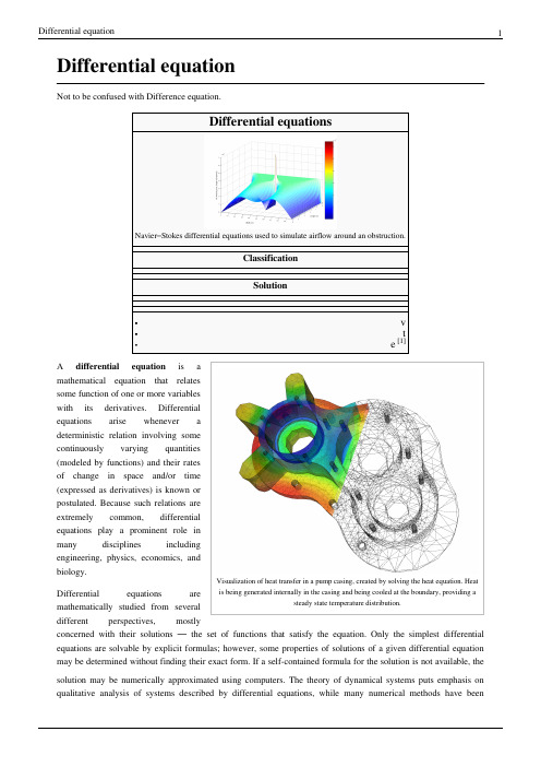
Differential equationNot to be confused with Difference equation.Stokes differential equations used to simulate airflow around an obstruction.ClassificationSolutionVisualization of heat transfer in a pump casing, created by solving the heat equation. Heat is being generated internally in the casing and being cooled at the boundary, providing a steady state temperature distribution.A differential equation is amathematical equation that relatessome function of one or more variableswith its derivatives. Differentialequations arise whenever adeterministic relation involving somecontinuously varying quantities(modeled by functions) and their ratesof change in space and/or time(expressed as derivatives) is known orpostulated. Because such relations areextremely common, differentialequations play a prominent role inmany disciplines includingengineering, physics, economics, andbiology.Differential equations aremathematically studied from severaldifferent perspectives, mostlyconcerned with their solutions — the set of functions that satisfy the equation. Only the simplest differential equations are solvable by explicit formulas; however, some properties of solutions of a given differential equation may be determined without finding their exact form. If a self-contained formula for the solution is not available, the solution may be numerically approximated using computers. The theory of dynamical systems puts emphasis on qualitative analysis of systems described by differential equations, while many numerical methods have beendeveloped to determine solutions with a given degree of accuracy.ExampleFor example, in classical mechanics, the motion of a body is described by its position and velocity as the time value varies. Newton's laws allow one (given the position, velocity, acceleration and various forces acting on the body) to express these variables dynamically as a differential equation for the unknown position of the body as a function of time.In some cases, this differential equation (called an equation of motion) may be solved explicitly.An example of modelling a real world problem using differential equations is the determination of the velocity of a ball falling through the air, considering only gravity and air resistance. The ball's acceleration towards the ground is the acceleration due to gravity minus the acceleration due to air resistance. Gravity is considered constant, and air resistance may be modeled as proportional to the ball's velocity. This means that the ball's acceleration, which is a derivative of its velocity, depends on the velocity (and the velocity depends on time). Finding the velocity as a function of time involves solving a differential equation and verifying its validity.Directions of studyThe study of differential equations is a wide field in pure and applied mathematics, physics, and engineering. All of these disciplines are concerned with the properties of differential equations of various types. Pure mathematics focuses on the existence and uniqueness of solutions, while applied mathematics emphasizes the rigorous justification of the methods for approximating solutions. Differential equations play an important role in modelling virtually every physical, technical, or biological process, from celestial motion, to bridge design, to interactions between neurons. Differential equations such as those used to solve real-life problems may not necessarily be directly solvable, i.e. do not have closed form solutions. Instead, solutions can be approximated using numerical methods.Mathematicians also study weak solutions (relying on weak derivatives), which are types of solutions that do not have to be differentiable everywhere. This extension is often necessary for solutions to exist.The study of the stability of solutions of differential equations is known as stability theory.NomenclatureThe theory of differential equations is well developed and the methods used to study them vary significantly with the type of the equation.Ordinary and partial•An ordinary differential equation (ODE) is a differential equation in which the unknown function (also known as the dependent variable) is a function of a single independent variable. In the simplest form, the unknown function is a real or complex valued function, but more generally, it may be vector-valued or matrix-valued: this corresponds to considering a system of ordinary differential equations for a single function.Ordinary differential equations are further classified according to the order of the highest derivative of the dependent variable with respect to the independent variable appearing in the equation. The most important cases for applications are first-order and second-order differential equations. For example, Bessel's differential equation(in which y is the dependent variable) is a second-order differential equation. In the classical literature a distinction is also made between differential equations explicitly solved with respect to the highest derivative and differential equations in an implicit form. Also important is the degree, or (highest) power, of the highest derivative(s) in the equation (cf. : degree of a polynomial). A differential equation is called a nonlinear differential equation if its degree is not one (a sufficient but unnecessary condition).• A partial differential equation (PDE) is a differential equation in which the unknown function is a function of multiple independent variables and the equation involves its partial derivatives. The order is defined similarly to the case of ordinary differential equations, but further classification into elliptic, hyperbolic, and parabolic equations, especially for second-order linear equations, is of utmost importance. Some partial differentialequations do not fall into any of these categories over the whole domain of the independent variables and they are said to be of mixed type.Linear and non-linearBoth ordinary and partial differential equations are broadly classified as linear and nonlinear.• A differential equation is linear if the unknown function and its derivatives appear to the power 1 (products of the unknown function and its derivatives are not allowed) and nonlinear otherwise. The characteristic property of linear equations is that their solutions form an affine subspace of an appropriate function space, which results in much more developed theory of linear differential equations. Homogeneous linear differential equations are a further subclass for which the space of solutions is a linear subspace i.e. the sum of any set of solutions or multiples of solutions is also a solution. The coefficients of the unknown function and its derivatives in a linear differential equation are allowed to be (known) functions of the independent variable or variables; if these coefficients are constants then one speaks of a constant coefficient linear differential equation.•There are very few methods of solving nonlinear differential equations exactly; those that are known typically depend on the equation having particular symmetries. Nonlinear differential equations can exhibit verycomplicated behavior over extended time intervals, characteristic of chaos. Even the fundamental questions of existence, uniqueness, and extendability of solutions for nonlinear differential equations, and well-posedness of initial and boundary value problems for nonlinear PDEs are hard problems and their resolution in special cases is considered to be a significant advance in the mathematical theory (cf. Navier–Stokes existence and smoothness).However, if the differential equation is a correctly formulated representation of a meaningful physical process, then one expects it to have a solution.Linear differential equations frequently appear as approximations to nonlinear equations. These approximations are only valid under restricted conditions. For example, the harmonic oscillator equation is an approximation to the nonlinear pendulum equation that is valid for small amplitude oscillations (see below).ExamplesIn the first group of examples, let u be an unknown function of x, and c and ω are known constants.•Inhomogeneous first-order linear constant coefficient ordinary differential equation:•Homogeneous second-order linear ordinary differential equation:•Homogeneous second-order linear constant coefficient ordinary differential equation describing the harmonic oscillator:•Inhomogeneous first-order nonlinear ordinary differential equation:•Second-order nonlinear (due to sine function) ordinary differential equation describing the motion of a pendulum of length L:In the next group of examples, the unknown function u depends on two variables x and t or x and y.•Homogeneous first-order linear partial differential equation:•Homogeneous second-order linear constant coefficient partial differential equation of elliptic type, the Laplace equation:•Third-order nonlinear partial differential equation, the Korteweg–de Vries equation:Related concepts• A delay differential equation (DDE) is an equation for a function of a single variable, usually called time, in which the derivative of the function at a certain time is given in terms of the values of the function at earlier times.• A stochastic differential equation (SDE) is an equation in which the unknown quantity is a stochastic process and the equation involves some known stochastic processes, for example, the Wiener process in the case of diffusion equations.• A differential algebraic equation (DAE) is a differential equation comprising differential and algebraic terms, given in implicit form.Connection to difference equationsSee also: Time scale calculusThe theory of differential equations is closely related to the theory of difference equations, in which the coordinates assume only discrete values, and the relationship involves values of the unknown function or functions and values at nearby coordinates. Many methods to compute numerical solutions of differential equations or study the properties of differential equations involve approximation of the solution of a differential equation by the solution of a corresponding difference equation.Universality of mathematical descriptionMany fundamental laws of physics and chemistry can be formulated as differential equations. In biology and economics, differential equations are used to model the behavior of complex systems. The mathematical theory of differential equations first developed together with the sciences where the equations had originated and where the results found application. However, diverse problems, sometimes originating in quite distinct scientific fields, may give rise to identical differential equations. Whenever this happens, mathematical theory behind the equations can be viewed as a unifying principle behind diverse phenomena. As an example, consider propagation of light and sound in the atmosphere, and of waves on the surface of a pond. All of them may be described by the same second-order partial differential equation, the wave equation, which allows us to think of light and sound as forms of waves, much like familiar waves in the water. Conduction of heat, the theory of which was developed by Joseph Fourier, is governed by another second-order partial differential equation, the heat equation. It turns out that many diffusion processes, while seemingly different, are described by the same equation; the Black–Scholes equation in finance is, for instance, related to the heat equation.Notable differential equationsPhysics and engineering•Newton's Second Law in dynamics (mechanics)•Euler–Lagrange equation in classical mechanics•Hamilton's equations in classical mechanics•Radioactive decay in nuclear physics•Newton's law of cooling in thermodynamics•The wave equation•Maxwell's equations in electromagnetism•The heat equation in thermodynamics•Laplace's equation, which defines harmonic functions•Poisson's equation•Einstein's field equation in general relativity•The Schrödinger equation in quantum mechanics•The geodesic equation•The Navier–Stokes equations in fluid dynamics•The Diffusion equation in stochastic processes•The Convection–diffusion equation in fluid dynamics•The Cauchy–Riemann equations in complex analysis•The Poisson–Boltzmann equation in molecular dynamics•The shallow water equations•Universal differential equation•The Lorenz equations whose solutions exhibit chaotic flow.Biology•Verhulst equation – biological population growth•von Bertalanffy model – biological individual growth•Lotka–Volterra equations – biological population dynamics•Replicator dynamics – found in theoretical biology•Hodgkin–Huxley model – neural action potentialsEconomics•The Black–Scholes PDE•Exogenous growth model•Malthusian growth model•The Vidale–Wolfe advertising modelReferences•P. Abbott and H. Neill, Teach Yourself Calculus, 2003 pages 266-277•P. Blanchard, R. L. Devaney, G. R. Hall, Differential Equations, Thompson, 2006• E. A. Coddington and N. Levinson, Theory of Ordinary Differential Equations, McGraw-Hill, 1955• E. L. Ince, Ordinary Differential Equations, Dover Publications, 1956•W. Johnson, A Treatise on Ordinary and Partial Differential Equations[2], John Wiley and Sons, 1913, in University of Michigan Historical Math Collection [3]• A. D. Polyanin and V. F. Zaitsev, Handbook of Exact Solutions for Ordinary Differential Equations (2nd edition), Chapman & Hall/CRC Press, Boca Raton, 2003. ISBN 1-58488-297-2.•R. I. Porter, Further Elementary Analysis, 1978, chapter XIX Differential Equations•Teschl, Gerald (2012). Ordinary Differential Equations and Dynamical Systems[4]. Providence: American Mathematical Society. ISBN 978-0-8218-8328-0.• D. Zwillinger, Handbook of Differential Equations (3rd edition), Academic Press, Boston, 1997.[1]/w/index.php?title=Template:Differential_equations&action=edit[2]/cgi/b/bib/bibperm?q1=abv5010.0001.001[3]/u/umhistmath/[4]http://www.mat.univie.ac.at/~gerald/ftp/book-ode/External links•Lectures on Differential Equations (/courses/mathematics/18-03-differential-equations-spring-2010/video-lectures/) MIT Open CourseWare Videos•Online Notes / Differential Equations (/classes/de/de.aspx) Paul Dawkins, Lamar University•Differential Equations (/diffeq/diffeq.html), S.O.S. Mathematics•Differential Equation Solver (/tools/differential_equation_solver/) Java applet tool used to solve differential equations.•Introduction to modeling via differential equations (/mat/u-u/en/ differential_equations_intro.htm) Introduction to modeling by means of differential equations, with critical remarks.•Mathematical Assistant on Web (http://user.mendelu.cz/marik/maw/index.php?lang=en&form=ode) Symbolic ODE tool, using Maxima•Exact Solutions of Ordinary Differential Equations (http://eqworld.ipmnet.ru/en/solutions/ode.htm)•Collection of ODE and DAE models of physical systems (/research/models.htm) MATLAB models•Notes on Diffy Qs: Differential Equations for Engineers (/diffyqs/) An introductory textbook on differential equations by Jiri Lebl of UIUC•Khan Academy Video playlist on differential equations (/math/ differential-equations) Topics covered in a first year course in differential equations.•MathDiscuss Video playlist on differential equations (/category/courses/ solutions-differential-equations/homogeneous-linear-systems/)Article Sources and Contributors8Article Sources and ContributorsDifferential equation Source: /w/index.php?oldid=610771276 Contributors: 17Drew, After Midnight, Ahoerstemeier, Alarius, Alfred Centauri, Amahoney, AndreiPolyanin, Andres, AndrewHowse, Andycjp, Andytalk, AngryPhillip, Anonymous Dissident, Antoni Barau, Antonius Block, Anupam, Apmonitor, Arcfrk, Asdf39, Asyndeton, Attilios,Babayagagypsies, Baccala@, Baccyak4H, Bejohns6, Bento00, Berland, Bidabadi, Bigusbry, BillyPreset, Bob.v.R, Bolatbek, Brandon, Bryanmcdonald, Btyner, Bygeorge2512,Callumds, Charles Matthews, Christian75, Chtito, Cispyre, Cmprince, Coginsys, ConMan, Cxz111, Cybercobra, DAJF, Danski14, Dbroadwell, Ddxc, Delaszk, DerHexer, Dewritech, Difu Wu, Djordjes, DominiqueNC, Donludwig, Dpv, Dr sarah madden, Drmies, DroEsperanto, Duoduoduo, Dysprosia, EconoPhysicist, Elwikipedista, Epicgenius, EricBright, Erin.Annette.Brown,Estudiarme, F=q(E+v^B), Fintor, Fioravante Patrone, Fioravante Patrone en, Flameturtle, Friend of the Facts, FutureTrillionaire, Gabrielleitao, Gandalf61, Gauss, Genedronek, Geni, Giftlite,GoingBatty, Gombang, Grenavitar, Haham hanuka, Hamiltondaniel, Harry, Haruth, Haseeb Jamal, Heikki m, Holmes1900, Ilya Voyager, Iquseruniv, Iulianu, Izodman2012, J arino, J.delanoy, Ja 62, Jak86, JamesBWatson, Jao, Jarble, Jauhienij, Jayden54, Jeancey, Jersey Devil, Jim Sukwutput, Jim.belk, Jim.henderson, JinJian, Jitse Niesen, JohnOwens, Johndoeisnotmyname, JorisvS,Julesd, K-UNIT, Kayvan45622, KeithJonsn, Kensaii, Khalid Mahmood, Klaas van Aarsen, Kr5t, Krushia, LOL, Lambiam, Lavateraguy, Lethe, LibLord, Linas, Lumos3, Madmath789, Mandarax, Mankarse, MarSch, Martastic, Martynas Patasius, Maschen, Math.geek3.1415926, Matqkks, Mattmnelson, Maurice Carbonaro, Maxis ftw, Mazi, McVities, Mduench, Mets501, Mh, MichaelHardy, Mindspillage, MisterSheik, Mohan1986, Mossaiby, Mpatel, MrOllie, Mtness, Mysidia, Nik-renshaw, Nkayesmith, Norm mit, Okopecz, Oleg Alexandrov, Opelio, Pahio, Parusaro, Paul August, Paul Matthews, Paul Richter, PavelSolin, Pgk, Phoebe, Pine, Pinethicket, Pratyya Ghosh, PseudoSudo, Qwerty Binary, Qzd800, R'n'B, Rama's Arrow, Randomguess, Reallybored999, RexNL, Reyk, RichMorin, Robin S, Romansanders, Rosasco, Ruakh, SDC, SFC9394, SakeUPenn, Salix alba, Sam Staton, Sampathsris, Sardanaphalus, Senoreuchrestud, Silly rabbit, Siroxo,Skakkle, Skypher, SmartPatrol, Snowjeep, Spirits in the Material, Starwiz, Suffusion of Yellow, Sverdrup, Symane, TVBZ28, TYelliot, Tannkrem, Tbhotch, Tbsmith, TexasAndroid, Tgeairn, The Hybrid, The Thing That Should Not Be, Timelesseyes, Tranum1234567890, Tsirel, Tuseroni, User A1, Vanished User 0001, Vishwanathnm, Vthiru, Waffleguy4, Waldir, Waltpohl, Wavelength, Wclxlus, Wihenao, Willtron, Winterheart, Wsears, XJaM, Yafujifide, Zepterfd, ﺪﺟﺎﺳ ﺪﺠﻣﺍ ﺪﺟﺎﺳ, 363 anonymous editsImage Sources, Licenses and ContributorsFile:Airflow-Obstructed-Duct.png Source: /w/index.php?title=File:Airflow-Obstructed-Duct.png License: Public Domain Contributors: Original uploader was User A1 at en.wikipediaFile:Elmer-pump-heatequation.png Source: /w/index.php?title=File:Elmer-pump-heatequation.png License: Creative Commons Attribution-Sharealike 3.0Contributors: Christian1985, Crimerob, Kri, User A1, 2 anonymous editsLicenseCreative Commons Attribution-Share Alike 3.0///licenses/by-sa/3.0/。
simultaneous equation method
Simultaneous Equation MethodIntroductionIn mathematics, simultaneous equations play a crucial role in solving real-world problems and modeling various phenomena. The simultaneous equation method is a powerful technique used to find solutions for a system of equations. This method involves solving multiple equations together to determine the values of unknown variables. In this article, we will explore the simultaneous equation method in detail and discuss its applications.Understanding Simultaneous EquationsDefinitionSimultaneous equations, also known as a system of equations, are a set of equations that share the same variables. The solutions of these equations simultaneously satisfy each equation in the system. The general form of simultaneous equations can be written as:a1x + b1y = c1a2x + b2y = c2Here, x and y are the variables, while a1, a2, b1, b2, c1, and c2 are constants.Types of Simultaneous EquationsSimultaneous equations can be classified into three types based on the number of solutions they have:1.Consistent Equations: These equations have a unique solution,meaning there is a specific set of values for the variables thatsatisfy all the equations in the system.2.Inconsistent Equations: This type of system has no solution. Theequations are contradictory and cannot be satisfied simultaneously.3.Dependent Equations: In this case, the system has infinitely manysolutions. The equations are dependent on each other and represent the same line or plane in geometric terms.To solve simultaneous equations, we employ various methods, with the simultaneous equation method being one of the most commonly used techniques.The Simultaneous Equation MethodThe simultaneous equation method involves manipulating and combining the given equations to eliminate one variable at a time. By eliminating one variable, we can reduce the system to a single equation with one variable, making it easier to find the solution.ProcedureThe general procedure for solving simultaneous equations using the simultaneous equation method is as follows:1.Identify the unknow n variables. Let’s assume we have n variables.2.Write down the given equations.3.Choose two equations and eliminate one variable by employingsuitable techniques such as substitution or elimination.4.Repeat step 3 until you have a single equation with one variable.5.Solve the single equation to determine the value of the variable.6.Substitute the found value back into the other equations to obtainthe values of the remaining variables.7.Verify the solution by substituting the found values into all theoriginal equations. The values should satisfy each equation.If the system is inconsistent or dependent, the simultaneous equation method will also lead to appropriate conclusions.Applications of Simultaneous Equation MethodThe simultaneous equation method finds applications in numerous fields, including:EngineeringSimultaneous equations are widely used in engineering to model and solve various problems. Engineers employ this method to determine unknown quantities in electrical circuits, structural analysis, fluid mechanics, and many other fields.EconomicsIn economics, simultaneous equations help analyze the relationship between different economic variables. These equations assist in studying market equilibrium, economic growth, and other economic phenomena.PhysicsSimultaneous equations are a fundamental tool in physics for solving complex problems involving multiple variables. They are used in areas such as classical mechanics, electromagnetism, and quantum mechanics.OptimizationThe simultaneous equation method is utilized in optimization techniques to find the optimal solution of a system subject to certain constraints. This is applicable in operations research, logistics, and resource allocation problems.ConclusionThe simultaneous equation method is an essential mathematical technique for solving systems of equations. By employing this method, we can find the values of unknown variables and understand the relationships between different equations. The applications of this method span across various fields, making it a valuable tool in problem-solving and modeling real-world situations. So, the simultaneous equation method continues to be akey topic in mathematics and its practical applications in diverse disciplines.。
西方哲学概论Descartes
“I shall consider myself as not having hands or eyes, or flesh, or blood or senses, but as falsely believing that I have all these things”
Second Meditation
2学时 2学时 2学时 2学时 2学时 2学时 2学时 2学时
Reference Books
Miller, Alexander. 2007 (2nd edition).
Philosophy of Language. UCL Press. Morris, Michael. 2007. An Introduction to the
Proof of the existence of God
Two important principles
Every thing has a cause “There must be at least as much reality in
the efficient and total cause as in the effect of that cause”
Meditations on First Philosophy (1641)
Brief account of Meditations Summary
I. Introducing Descartes
TheKlein-Gordonequation:克莱因戈登方程
where the Lagrangian density satisfies the Euler-Lagrange equations of motions
(25)
such that the Euler-Lagrange equations of motion just give the Klein-Gordon equation (12) and its complex conjugate.
as the basic field equation of the scalar field.
The plane waves (10) are basic solutions and the field (9) is constructed by
a general superposition of the basic states.
Quantization
The challenge is to find operator solutions of the Klein-Gordon equation (12) which satisfy eq. (28). In analogy to the Lagrange density (24) , the hamiltonian is
Lecture 8
The Klein-Gordon equation
WS2010/11: ‚Introduction to Nuclear and Particle Physics‘
The bosons in field theory
Bosons with spin 0
scalar (or pseudo-scalar) meson fields
(23)
Chapter 6 - Solid Solutions
Solid Solutions
22. P A I R P R O B A B I L I T Y F U N C T I O N S : THERMODYNAMIC PROPERTIES
A solid phase containing two or more kinds of atom, the relative proportions of which may be varied within limits, is described as a solid solution. Terminal solid solutions are based on the structures of the component metals; intermediate solid solutions may have structures which are different from any of those of the constituents. Most solid solutions are of the substitutional type, in which the different atoms are distributed over one or more sets of common sites, and may interchange positions on the sites. In interstitial solutions, the solute atoms occupy sites in the spaces between the positions of the atoms of the solvent metal; this can only happen when the solute atoms are much smaller than the atoms of the solvent. We must also distinguish between ordered and disordered solid solutions. In the fully ordered state each set of atoms occupies one set of positions, so that the atomic arrangement is similar to that of a compound. This is only possible at compositions where the ratios of the numbers of atoms of different kinds are small integral numbers, but the atomic arrangement may still be predominantly ordered in this way for alloys of arbitrary composition. In disordered solid solutions, the atoms are distributed among the sites they occupy in a nearly random manner. This classification is only approximate, and we shall formulate these concepts more precisely. The definition of the unit cell, and the concept of the translational periodicity of the lattice, lose their strict validity when applied to a disordered solid solution. The mean positions of the atoms, considered as mathematical points, will no longer be specified exactly by (5.8), since there will be local distortions depending on the details of the local configurations. Moreover, a knowledge of the type of atom at one end of a given interatomic vector no longer implies knowledge of the atom at the other end, as it does for a pure component or a fully ordered structure. In a solid solution, precise statements of this nature have to be replaced by statements in terms of the probability of the atom being of a certain type. For many purposes, the strict non-periodicity of the structure is not important, since most physical properties are averages over reasonably large numbers of atoms. Thus the positions of X-ray diffraction maxima depend only on the average unit cell dime Theory of Transformations in Metals and Alloys
关于数字的英语作文

In the realm of English composition,writing about numbers can be an engaging and informative task.Here are some key points to consider when crafting an essay on this topic:1.Introduction to the Significance of Numbers:Begin your essay by highlighting the importance of numbers in our daily lives,from counting to complex mathematical equations that drive scientific advancements.2.Historical Perspective:Discuss the evolution of numerical systems,such as the transition from Roman numerals to the Arabic numerals we use today.This can provide an interesting historical context.3.Cultural Impact:Numbers hold different significance in various cultures.For example, the number13is considered unlucky in Western cultures,while in some Asian cultures, the number4is associated with death.4.Mathematical Concepts:Delve into fundamental mathematical concepts related to numbers,such as prime numbers,factorials,and Fibonacci sequences.Explain how these concepts are applied in realworld scenarios.5.The Role of Numbers in Science:Explore how numbers are integral to scientific theories and formulas.For instance,the use of piπin calculating the circumference of a circle or the golden ratio in art and architecture.6.Numerical Systems in Technology:Discuss binary and hexadecimal systems used in computer programming and how they differ from the decimal system.7.Statistics and Data Analysis:Numbers play a crucial role in statistics,allowing us to make sense of large data sets,draw conclusions,and make predictions.8.Personal Finance and Economics:Numbers are the backbone of financial systems, from calculating interest rates to understanding economic indicators like GDP and inflation.9.The Beauty of Numbers in Art and Literature:Some authors and artists use numbers creatively in their works,either as themes or structural elements.For example,the use of numerical patterns in poetry or the significance of certain numbers in novels.10.The Future of Numbers:Conclude your essay by speculating on the future of numbers, including potential advancements in mathematics,the role of artificial intelligence innumber theory,and how our understanding and use of numbers may evolve. Remember to use clear examples and explanations to illustrate your points,and ensure that your essay flows logically from one section to the next.Writing about numbers can be both educational and enjoyable,offering a window into the universal language that connects us all.。
- 1、下载文档前请自行甄别文档内容的完整性,平台不提供额外的编辑、内容补充、找答案等附加服务。
- 2、"仅部分预览"的文档,不可在线预览部分如存在完整性等问题,可反馈申请退款(可完整预览的文档不适用该条件!)。
- 3、如文档侵犯您的权益,请联系客服反馈,我们会尽快为您处理(人工客服工作时间:9:00-18:30)。
. . . . .
. . . . .
. . . . .
. . . . .
. . . . .
. . . . .
. . . . .
. . . . .
. . . . .
. . . . .
. . . . .
. . . . .
. . . . .
. . . . . . . . . . . . . . . . . . . . . . . . . . . . . . . . . . .
2
Abstract Understanding, finding, or even deciding on the existence of real solutions to a system of equations is a very difficult problem with many applications. While it is hopeless to expect much in general, we know a surprising amount about these questions for systems which possess additional structure. Particularly fruitful—both for information on real solutions and for applicability—are systems whose additional structure comes from geometry. Such equations from geometry for which we have information about their real solutions will be the subject of this short course. We will focus on equations from toric varieties and homogeneous spaces, particularly Grassmannians. Not only is much known in these cases, but they encompass some of the most common applications. The results we discuss may be grouped into three themes: (I) Upper bounds on the number of real solutions. (II) Geometric problems that can have all solutions be real. (III) Lower bounds on the number of real solutions. Upper bounds as in (I) bound the complexity of the set of real solutions—they are one of the sources for the theory of o-minimal structures which are an important topic in real algebraic geometry. The existence (II) of geometric problems that can have all solutions be real was initially surprising, but this phenomena now appears ubiquitous. Lower bounds as in (III) give an existence proof for real solutions. Their most spectacular manifestation is the non-triviality of the Welschinger invariant, which was computed via tropical geometry. I first thank the Institut Henri Poincar´ e, where these lectures took place and where I resided during much of their development. Also Prof. Dr. Peter Gritzmann of the Technische Universit¨ at M¨ unchen, whose hospitality enabled the completion of these notes. Lastly, I thank the students, both young and old, who attended the lectures.
49 54 54 54 57 58 61 61 63 66 68
7 The Shapiro Conjecture for Rational Functions 7.1 The Shapiro Conjecture for rational functions . . 7.1.1 Preliminaries on rational functions . . . . 7.1.2 Schubert induction and the proof . . . . . 7.1.3 Main theorem and completion of the proof 8 Beyond the Shapiro Conjecture 8.1 Transversality . . . . . . . . . . . . . . . . 8.2 Maximally inflected curves . . . . . . . . . 8.3 The Shapiro Conjecture for flag manifolds 8.3.1 The Monotone Conjecture . . . . . . . . . . . . . . . . . . . . .
6.2.1
Schubert varieties . . . . . . . . . . . . . . . . . . . . . . . . . . . . . . . . . . . . . . . . . . . . . . . . . . . . . . . . . . . . . . . . . . . . . . . . . . . . . . . . . . . . . . . . . . . . . . . . . . . . . . . . . . . . . . . . . . . . . . . . . . . . . . . . . . . . . . . . . . . . . . . . . . . . .
5 March 2006
1 Overview 1.1 Upper bounds . . . . . . . . . . . . . . . . . . . . 1.2 The Wronski map and Shapiro’s Conjecture . . . 1.2.1 The problem of four lines . . . . . . . . . . 1.2.2 Rational functions with real critical points 1.3 Lower bounds . . . . . . . . . . . . .. . . . . . . . . . . . . . . . . . . . . . . . . . . .
1 3 4 5 6 6 10 11 12 15 15 17 19 20 21 21 25 26 27 27 28 30 31 33 34 35 36 36 37 37 38 39 39 41 42 43 45 45 46 47 48
Theorem . . . . . . . . . . . . . . . . . . . . . . . . . . . . . . . . . . . . . . . . . . . . . . . . . . . . . . . . . . . . . . . . . . . . . . . . . . . . . . . . . . . . . . . . . . . . . . . . . . . . . . . . . . . . . . . . . . . . . . . . . . . . . . . . . . . . . . . . . . . . . . . . . . . . . . . . . . . . . . . . . . . . . . . . . . . . . .
2 Sparse Polynomial Systems 2.1 The geometry of sparse polynomial systems and Kushnirenko’s 2.1.1 Algebraic-geometric proof of Kushnirenko’s Theorem . 2.2 Algorithmic proof of Kushnirenko’s Theorem . . . . . . . . . . 2.2.1 The case of a simplex . . . . . . . . . . . . . . . . . . . 2.2.2 Regular triangulations and toric deformations . . . . . 2.2.3 Kushnirenko’s Theorem via toric deformations . . . . . 2.2.4 A brief aside about real solutions . . . . . . . . . . . . 3 Upper Bounds 3.1 Khovanskii’s fewnomial bound . . . . . . . . . . 3.1.1 Kushnirenko’s (non) conjecture . . . . . 3.2 Systems supported on a circuit . . . . . . . . . 3.2.1 Some arithmetic for circuits . . . . . . . 3.2.2 Elimination for circuits . . . . . . . . . . 3.2.3 A family of systems with a sharp bound 4 Lower Bounds for Sparse Polynomial Systems 4.1 Polynomial systems from posets . . . . . . . . . 4.2 Orientability of real toric varieties . . . . . . . . 4.3 Degree from balanced triangulations . . . . . . . 4.4 Reprise: polynomial systems from posets . . . . 4.5 Sagbi degenerations . . . . . . . . . . . . . . . . 4.6 Future directions . . . . . . . . . . . . . . . . . . . . . . . . . . . . . . . . . . . . . . . . . . . . . . . . . . . . . . . . . . . . . . . . . . . . . . . . . . . . . . . . . . . . . . . . . . . . . . . . . . . . . . . . . . . . . . . . . . . . . . . . . . . . . . . . . . . . . . . . . . . . . . . . . . . . . . . . . . . . . . . . . . . . . . . .