The GraF instrument for imaging spectroscopy with the adaptive optics
光谱仪器原理
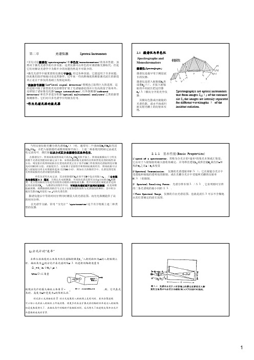
Spectrographys are optical instruments that form images S2(λ) of the entrance slit S1;the images are laterally separated for different wavelengths λof the incident radiation.Ω=F/f12受棱镜的有效面积F=h.a的限制,它代表光的限制孔径.的方式成像到入射狭缝上是有利的,虽然会聚透镜可以缩小光源在入射狭经上所成的像,使更多的来自扩展光源的辐射功率通过入射狭缝:但是发散度增大了.在接收角外的辐射不能被探测到,反而增大了由透镜支架和分光计任何色散型仪器的光谱分辨本领的定义为和λ2间的最小间隔.-λ2)在二个最大间显示出明显的凹陷,则可以认为强度分布是由具有强度轮廓为I1(λ-λ1)和I21(λ-λ2)的二条)依赖于比率I1/I2和二个分量的轮廓,因此最小对于不同的轮廓将是不相同.2的第一最小重合,则认为两条谱线如果强度相等的两条线的两个最大间的凹陷降到I的(8/π2)≈0.8,(a)Diffraction in a spectrometer by the limiting aperture with diameter af1f2:angular dispersion[rad/nm]成像在平面B上)间的距离△x2为=(dx/dλ)△λ:linear dispersion of the instrument,[mm/nm]为了分辨λ和λ+△λ的二条线,上式中的间距△x2至少应为二个狭缝象的宽度(λ)+δx2(λ+△λ),由于宽度x2由下式与入射狭缝宽度相联系:δx2=(f2/f1) δx1所以减小δx1便能增大分辨本领λ/△λ,可惜存在着由衍射造成的理论极限.由于分辨极限十分重要.我们将对这点作更详细的讨论.(b)Limitation of spectral resolution by diffraction=±λ/b间(见图);仅当2 δΦ小于分光计的接收角a/f1时,它才能完全通过限制孔径a.这给出入射狭缝有效宽度bmin的下限为在一切实际情形中,入射光都是发散的.这就要求发散角和衍射角之和必须小于,而最小狭缝相应地更大。
肌骨超声联合CT_能谱成像在不同临床时期痛风患者诊断中的敏感度和准确性分析

肌骨超声联合CT能谱成像在不同临床时期痛风患者诊断中的敏感度和准确性分析*黄海霞① 温小芳① 彭诚初① 黄旭胜① 【摘要】 目的:研究肌骨超声联合CT能谱成像在痛风患者不同临床时期的应用价值。
方法:回顾性分析2021年1月—2023年6月在广州医科大学附属惠州医院超声科进行肌骨超声检查、CT能谱检查的66例疑似痛风患者的临床资料。
以关节穿刺和镜检尿酸单钠晶体为诊断“金标准”,对比单一肌骨超声、CT能谱成像诊断和二者联合诊断对痛风的诊断效能(敏感度、准确性)及对痛风不同临床时期的诊断符合率(急性期、间歇发作期、慢性关节炎期)。
结果:肌骨超声联合CT能谱成像的诊断敏感度(100%)、准确性(96.97%)均高于单一肌骨超声(85.96%、77.27%)、CT能谱成像(89.47%、81.82%)(P<0.05)。
肌骨超声联合CT能谱成像对急性期、间歇发作期、慢性关节炎期的诊断符合率均高于单一肌骨超声、CT能谱成像(P<0.05)。
结论:在痛风患者中采用肌骨超声联合CT能谱成像诊断,能提高诊断敏感度、准确性,并明确患者的临床时期,在临床治疗中具有重要指导价值。
【关键词】 痛风 临床时期 肌骨超声 CT能谱成像 敏感度 准确性 Sensitivity and Accuracy Analysis of Muscle Bone Ultrasound Combined with CT Energy SpectrumImaging in Different Clinical Stages of Gout Patients/HUANG Haixia, WEN Xiaofang, PENG Chengchu,HUANG Xusheng. //Medical Innovation of China, 2024, 21(10): 097-100 [Abstract] Objective: To study the application value of muscle bone ultrasound combined with CT energyspectrum imaging in different clinical stages of gout patients. Method: A retrospective analysis was conducted onthe clinical data of 66 patients with suspected gout who underwent muscle bone ultrasound and CT energy spectrumexamination in Huizhou Hospital Affiliated to Guangzhou Medical University from January 2021 to June 2023. Jointpuncture and microscopic examination of monosodium urate crystals were used as the diagnostic "gold standard",The diagnostic efficacy (sensitivity, accuracy) of and single muscle bone ultrasound, CT energy spectrum imagingdiagnosis and the combination of the two for gout were compared, as well as the diagnostic coincidence rate for goutat different clinical stages (acute stage, intermittent attack stage, chronic arthritis stage), while the muscle boneultrasound and CT energy spectrum imaging characteristics of gout patients at different clinical stages were analyzed.Result: The diagnostic sensitivity (100%) and accuracy (96.97%) of muscle bone ultrasound combined with CTenergy spectrum imaging were higher than those of single muscle bone ultrasound (85.96%, 77.27%) and CT energyspectrum imaging (89.47%, 81.82%) (P<0.05). The diagnostic accuracy of muscle bone ultrasound combined withCT energy spectrum imaging in acute stage, intermittent attack stage, and chronic arthritis stages was higher thanthose of single muscle bone ultrasound and CT energy spectrum imaging (P<0.05). Conclusion: The use of musclebone ultrasound combined with CT energy spectrum imaging in gout patients can improve diagnostic sensitivityand accuracy, and accurately determine the clinical period of the patient. It has important guiding value in clinicaltreatment. [Key words] Gout Clinical stage Muscle bone ultrasound CT energy spectrum imaging Sensitivity Accuracy First-author's address: Department of Ultrasound, Huizhou Hospital Affiliated to Guangzhou MedicalUniversity, Huizhou 516002, China doi:10.3969/j.issn.1674-4985.2024.10.022*基金项目:惠州市科技计划项目(210422114572931)①广州医科大学附属惠州医院(惠州市第三人民医院)超声科 广东 惠州 516002通信作者:黄海霞- 97 - 痛风是一种由嘌呤代谢失衡和/或尿酸排泄障碍而导致长期血尿酸增高、尿酸盐晶体广泛沉积引起的反复发作性炎症疾病[1-2]。
傅里叶变换红外光谱仪英文
傅里叶变换红外光谱仪英文Fourier Transform Infrared SpectrometerIntroduction:The Fourier Transform Infrared (FTIR) spectrometer is an essential tool in the field of spectroscopy. It utilizes the mathematical technique known as Fourier transform to analyze infrared light, enabling scientists to study the molecular composition and structure of various substances. In this article, we will explore the principles behind the Fourier Transform Infrared Spectrometer and its applications in scientific research.Principles of Fourier Transform Infrared Spectroscopy:Fourier Transform Infrared Spectroscopy is based on the interaction between infrared light and matter. When a substance is exposed to infrared radiation, the energy absorbed by the molecules causes them to vibrate. These vibrations are specific to each molecule and are dependent on the molecular bonds present within the substance.The spectrometer operates by passing an infrared beam through the sample and measuring the amount of light absorbed at different wavelengths. This absorption spectrum is then transformed using Fourier analysis, producing a highly detailed and accurate representation of the substance's molecular structure.Advantages of Fourier Transform Infrared Spectroscopy:1. High Speed and Sensitivity: Fourier Transform Infrared Spectroscopy offers rapid analysis times due to its ability to gather a full range ofwavelengths simultaneously. This allows for efficient data collection, making it ideal for high-throughput applications. Additionally, the technique is highly sensitive, capable of detecting even small quantities of sample material.2. Broad Analytical Range: FTIR spectroscopy covers a wide range of wavelengths, from near-infrared (NIR) to mid-infrared (MIR). This versatility enables the analysis of various substances, including organic and inorganic compounds, polymers, pharmaceuticals, and biological samples.3. Non-destructive Analysis: One of the key advantages of FTIR spectroscopy is that it is a non-destructive technique. Samples do not require any special preparation and can be analyzed directly, allowing for subsequent analysis or retesting if required.Applications of Fourier Transform Infrared Spectrometers:1. Pharmaceutical Analysis: FTIR spectroscopy plays a vital role in drug discovery and development. It is used to identify and characterize the molecular composition of active pharmaceutical ingredients (APIs), excipients, and impurities. By comparing spectra, scientists can ensure the quality and purity of pharmaceutical products.2. Environmental Analysis: Fourier Transform Infrared Spectrometers are employed in environmental monitoring to analyze air, water, and soil samples. It aids in detecting pollutants, identifying unknown substances, and assessing the impact of human activities on the environment.3. Forensic Science: FTIR spectroscopy has proven to be a valuable tool in forensic science. It assists in the analysis of various evidence, such asfibers, paints, and drugs. FTIR spectra can provide crucial information in criminal investigations, helping to identify unknown substances and link them to potential sources.4. Food and Beverage Industry: The FTIR spectrometer allows for the analysis of food quality, safety, and authenticity. It can identify contaminants, detect adulteration, and verify product labeling claims. Both raw materials and finished products can be analyzed using this technique, ensuring compliance with industry regulations.Conclusion:The Fourier Transform Infrared Spectrometer has revolutionized the field of spectroscopy by providing accurate and detailed information about a substance's molecular structure. Its speed, sensitivity, and versatility make it a crucial analytical tool in various scientific disciplines. With ongoing advancements in technology, FTIR spectroscopy continues to contribute to new discoveries and advancements in research.。
offner成像光谱仪的设计方法

offner成像光谱仪的设计方法英文回答:Designing an Offner imaging spectrometer involves several key steps and considerations. The Offner configuration is a popular choice for its compactness and ability to provide high spectral resolution. Here is a step-by-step guide to designing an Offner imaging spectrometer:1. Determine the spectral range and resolution requirements: The first step is to define the desired spectral range and resolution for the spectrometer. This will depend on the specific application and the types of samples or phenomena that need to be analyzed.2. Select the correct optics: The Offner configuration consists of two concave mirrors and a convex grating. The choice of optics is crucial to achieve the desired performance. The mirrors should have a high reflectivityand low scattering, while the grating should have a high diffraction efficiency and low stray light.3. Calculate the design parameters: The design parameters of the Offner spectrometer include the focal lengths of the mirrors, the radius of curvature of the grating, and the distance between the mirrors. These parameters need to be carefully calculated to ensure proper imaging and dispersion.4. Consider aberrations: Offner spectrometers are prone to various aberrations, such as astigmatism and coma. These aberrations can degrade the spectral and spatial resolution. It is important to analyze and minimize these aberrations through careful design and optimization.5. Optimize the system: Once the initial design is complete, it is necessary to optimize the system for better performance. This can involve adjusting the mirror curvatures, grating position, or other parameters toachieve the desired spectral resolution and image quality.6. Test and calibrate: After the design and optimization, the Offner spectrometer needs to be tested and calibrated. This involves measuring the spectral and spatial resolution, as well as characterizing any remaining aberrations or distortions. Calibration methods, such as using known spectral sources or calibration standards, can help ensure accurate measurements.7. Consider practical constraints: Finally, it is important to consider practical constraints in the design, such as size, weight, and cost. Offner spectrometers can be quite compact, but trade-offs may need to be made to meet specific requirements.中文回答:设计Offner成像光谱仪涉及到几个关键步骤和考虑因素。
可见光光谱 英文
可见光光谱英文The visible light spectrum, encompassing wavelengths ranging from approximately 400 nanometers (nm) to 700 nm,is a narrow slice of the electromagnetic radiation that our eyes are capable of perceiving. This band of wavelengths, although relatively small compared to the vast expanse of the electromagnetic spectrum, plays a pivotal role in our daily lives, shaping our perception of the world around us. At the shorter wavelength end of the visible spectrum, we encounter violet light. Violet waves, with their frequencies exceeding 668 THz, are the highest in energy among all visible colors. As we move towards the red end of the spectrum, wavelengths increase, resulting in lower frequencies and consequently, lower energy levels. Red light, with wavelengths exceeding 700 nm, has the lowest energy among all visible colors.The visible spectrum is not just a random assortment of colors; it is a carefully crafted array of hues that enables us to perceive a wide range of colors. The human eye is equipped with photoreceptors called cones, which are sensitive to specific wavelengths within the visiblespectrum. These cones are primarily sensitive to blue, green, and red light, allowing us to perceive the full range of colors visible to the naked eye.The importance of the visible light spectrum extends beyond our ability to see colors. It plays a crucial role in photosynthesis, the process by which plants convert light energy into chemical energy. Chlorophyll, the green pigment found in plants, is highly absorbent of blue and red light wavelengths, which are essential for photosynthesis. Without the visible light spectrum, photosynthesis would not be possible,严重影响着整个生态系统的运转。
傅里叶红外光谱仪英文

傅里叶红外光谱仪英文傅里叶红外光谱仪英文IntroductionFourier transform infrared spectroscopy (FTIR) is a powerful analytical technique used to identify the chemical composition of a sample based on its molecular vibrations. FTIR spectrometers have various ranges, including mid-infrared (MIR), near-infrared (NIR), and far-infrared (FIR). In this article, we will focus on the Fourier transform infrared spectrometer in the mid-infrared range, also known as FTIR-MIR.InstrumentationFTIR-MIR spectrometers consist of a light source, a sample compartment, a detector, and an interferometer. The interferometer is the heart of the FTIR instrument, as it converts the sample's spectral signal from a time domain to a frequency domain. The signal is then detected by a detector and processed through a computer. The main components of the MIR-FTIR spectrometer include:1. Light source: Typically, a high-intensity, high-resolution infrared source is used, such as a Globar or a mercury-cadmium-telluride (MCT) detector.2. Sample compartment: This is where the sample is placed for analysis. Samples can be in the form of liquids, solids, gases, or films.3. Interferometer: This is the key component of the FTIR-MIR spectrometer.There are several types of interferometers, including Michelson and Fourier transform.4. Detector: The detector is used to detect the spectral signal from the interferometer and generate an electrical signal that is then processed and displayed on the computer.ApplicationsFTIR-MIR spectrometers are widely used in various industries, including pharmaceuticals, chemistry, polymers, food, and environmental analysis. This technique is used to identify and characterize chemical compounds, determine the purity of samples, identify unknown compounds, and monitor chemical reactions. FTIR-MIR can also be used to detect and quantify gases and pollutants in the atmosphere.AdvantagesFTIR-MIR spectrometers have several advantages over other analytical techniques, including:1. Non-destructive analysis: FTIR-MIR analysis does not destroy the sample, allowing for further analysis if necessary.2. Fast analysis: The analysis time for FTIR-MIR is usually less than a minute, making it a quick and efficient technique for sample analysis.3. High sensitivity: FTIR-MIR spectrometers can detect trace amounts of compounds, making it possible to identify small impurities in a sample.4. Versatility: FTIR-MIR can be used to analyze a wide range of sample types, including liquids, solids, gases, and films.ConclusionFourier transform infrared spectrometry is a powerful analytical technique that can provide valuable information in various industries. With its non-destructive analysis, fast analysis time, high sensitivity, and versatility, FTIR-MIR spectrometers are essential tools for chemical analysis and pollution monitoring.。
荧光成像基础知识
12
SCHOOL of FLUORESCENCE
MPSF educator packet
This packet contains illustrations and figures from the Molecular Probes® School of Fluorescence website. They illustrate concepts from the basic physical properties that underlie fluorescence through experiment planning and troubleshooting. The images and graphics on this page are copyrighted, but they are freely available for your use as long as the attribution “Molecular Probes®” remains intact.
10
SCHOOL of FLUORESCENCE
Part One: Fundamentals of Fluorescence Microscopy
Figure 2.2. The light path through lenses and sample in basic brightfield microscopy (A). Antique 19th century drum-style compound microscope (B).
Figure 1.3. The inverse relationship between energy and wavelength in the visible spectrum.
纹理物体缺陷的视觉检测算法研究--优秀毕业论文
摘 要
在竞争激烈的工业自动化生产过程中,机器视觉对产品质量的把关起着举足 轻重的作用,机器视觉在缺陷检测技术方面的应用也逐渐普遍起来。与常规的检 测技术相比,自动化的视觉检测系统更加经济、快捷、高效与 安全。纹理物体在 工业生产中广泛存在,像用于半导体装配和封装底板和发光二极管,现代 化电子 系统中的印制电路板,以及纺织行业中的布匹和织物等都可认为是含有纹理特征 的物体。本论文主要致力于纹理物体的缺陷检测技术研究,为纹理物体的自动化 检测提供高效而可靠的检测算法。 纹理是描述图像内容的重要特征,纹理分析也已经被成功的应用与纹理分割 和纹理分类当中。本研究提出了一种基于纹理分析技术和参考比较方式的缺陷检 测算法。这种算法能容忍物体变形引起的图像配准误差,对纹理的影响也具有鲁 棒性。本算法旨在为检测出的缺陷区域提供丰富而重要的物理意义,如缺陷区域 的大小、形状、亮度对比度及空间分布等。同时,在参考图像可行的情况下,本 算法可用于同质纹理物体和非同质纹理物体的检测,对非纹理物体 的检测也可取 得不错的效果。 在整个检测过程中,我们采用了可调控金字塔的纹理分析和重构技术。与传 统的小波纹理分析技术不同,我们在小波域中加入处理物体变形和纹理影响的容 忍度控制算法,来实现容忍物体变形和对纹理影响鲁棒的目的。最后可调控金字 塔的重构保证了缺陷区域物理意义恢复的准确性。实验阶段,我们检测了一系列 具有实际应用价值的图像。实验结果表明 本文提出的纹理物体缺陷检测算法具有 高效性和易于实现性。 关键字: 缺陷检测;纹理;物体变形;可调控金字塔;重构
Keywords: defect detection, texture, object distortion, steerable pyramid, reconstruction
II
高光谱英文缩写
高光谱英文缩写Hyperspectral imaging, often referred to as HSI, is a powerful and versatile technology that has revolutionized the way we perceive and analyze the world around us. This advanced imaging technique goes beyond the capabilities of traditional digital cameras by capturing a vast array of spectral information from the electromagnetic spectrum, providing a wealth of data that can be used in a wide range of applications.At its core, hyperspectral imaging involves the acquisition of high-dimensional data cubes, where each pixel in the image contains a detailed spectral signature. This signature represents the unique reflectance or emission characteristics of the target material, allowing for the identification and classification of a wide variety of substances and materials. Unlike conventional RGB (red, green, blue) imaging, which captures only three color channels, hyperspectral sensors can record hundreds or even thousands of narrow spectral bands, creating a rich and detailed spectral profile.The power of hyperspectral imaging lies in its ability to revealinformation that is invisible to the human eye or traditional imaging techniques. By capturing the subtle nuances of the electromagnetic spectrum, HSI can detect and analyze a diverse range of materials, from minerals and vegetation to man-made objects and even chemical compounds. This capability has made it an indispensable tool in a variety of fields, including remote sensing, environmental monitoring, agriculture, and even medical diagnostics.In the realm of remote sensing, hyperspectral imaging has revolutionized the way we study and manage our natural resources. By analyzing the spectral signatures of different materials, researchers can map and monitor the distribution of minerals, identify areas of vegetation stress, and detect the presence of pollutants or contaminants in the environment. This information is invaluable for a wide range of applications, from mineral exploration and forestry management to environmental impact assessments and disaster response.In the agricultural sector, hyperspectral imaging has become a crucial tool for precision farming and crop monitoring. By analyzing the spectral signatures of plants, farmers can detect early signs of disease, nutrient deficiencies, or water stress, allowing them to take targeted action to improve crop yields and reduce the environmental impact of their operations. Additionally, HSI can be used to map soil composition, monitor crop growth, and even detect the presence ofpests or weeds, enabling more efficient and sustainable farming practices.The medical field has also benefited greatly from the advances in hyperspectral imaging technology. In the area of diagnostics, HSI has shown promise in the early detection of various diseases, such as skin cancer, breast cancer, and cardiovascular conditions. By analyzing the unique spectral signatures of diseased tissues, healthcare professionals can identify subtle changes that may not be visible to the naked eye, enabling earlier intervention and improved patient outcomes.Beyond these applications, hyperspectral imaging has found its way into numerous other industries, including art conservation, forensics, and even aerospace engineering. In the field of art conservation, HSI can be used to identify pigments, detect forgeries, and monitor the condition of valuable artworks, while in forensics, it has been employed to analyze trace evidence and identify illicit substances.As the technology continues to evolve, the potential applications of hyperspectral imaging are virtually limitless. With advancements in sensor technology, data processing, and analytical algorithms, the future of HSI looks increasingly bright, promising new discoveries and innovations that will shape our understanding of the world around us.However, the widespread adoption of hyperspectral imaging technology is not without its challenges. The sheer volume of data generated by HSI systems, coupled with the complexity of the spectral analysis, can pose significant computational and storage challenges. Additionally, the cost of the specialized equipment and the expertise required to interpret the data can be barriers to entry for some organizations and individuals.Despite these challenges, the benefits of hyperspectral imaging are clear, and the technology continues to gain traction across a wide range of industries and disciplines. As researchers and engineers work to overcome the technical hurdles, the future of HSI looks increasingly promising, with the potential to unlock new insights and discoveries that will shape our understanding of the world around us.In conclusion, hyperspectral imaging is a transformative technology that has the power to revolutionize the way we perceive and interact with our environment. By capturing the rich spectral information that lies beyond the visible spectrum, HSI has opened up new frontiers of scientific exploration and practical applications, from remote sensing and precision agriculture to medical diagnostics and forensic analysis. As the technology continues to evolve and become more accessible, the potential of hyperspectral imaging to drive innovation and improve our understanding of the world around us is truly limitless.。
核磁共振基本原理与实验操作指导说明书
Chapter 1: NMR Coupling ConstantsNMR can be used for more than simply comparing a product to a literature spectrum. There is a great deal of information that can be learned from analysis of the coupling constants for a compound.1.1Coupling Constants and the Karplus EquationWhen two protons couple to each other, they cause splitting of each other’s peaks. The spacing between the peaks is the same for both protons, and is referred to as the coupling constant or J constant. This number is always given in hertz (Hz), and is determined by the following formula:J Hz = ∆ ppm x instrument frequency∆ ppm is the difference in ppm of two peaks for a given proton. The instrument frequency is determined by the strength of the magnet, and will always be 300 MHz for all spectra collected on the organic teaching lab NMR.Figure 1-1 below shows the simulated NMR spectrum of 1,1-dichloroethane, collected in a 30 MHz instrument. This compound has coupling between A (the quartet at 6 ppm) and B (the doublet at 2 ppm).Figure 1-1: The NMR spectrum of 1,1-dichloroethane, collected in a 30 MHz instrument. For both A and B protons, the peaks are spaced by 0.2 ppm, equal to 6 Hz in this instrument.For both A and B, the distance between the peaks is equal. In this example, the spacing between the peaks is 0.2 ppm (for example, the peaks for A are at 6.2, 6.0, 5.8, and 5.6 ppm). This is equal to a J constant of (0.2 ppm • 30 MHz) = 6 Hz. Since the shifts are given in ppm or parts per million, you should divide by 106. But since the frequency is in megahertz instead of hertz, you should multiply by 106. These two factors cancel each other out, making calculations nice and simple.Figure 1-2 below shows the NMR spectrum of the same compound, but this time collected in a 60 MHz instrument.Chapter 1: NMR Coupling ConstantsFigure 1-2: The NMR spectrum of 1,1-dichloroethane, collected in a 60 MHz instrument. For both A and B protons, the peaks are spaced by 0.1 ppm, equal to 6 Hz in this instrument.This time, the peak spacing is 0.1 ppm. This is equal to a J constant of (0.1 ppm • 60 MHz) = 6 Hz, the same as before. This shows that the J constant for any two particular protons will be the same value in hertz, no matter which instrument is used to measure it.The coupling constant provides valuable information about the structure of a compound. Some typical coupling constants are shown here.Figure 1-3: The coupling constants for some typical pairs of protons.In molecules where the rotation of bonds is constrained (for instance, in double bonds or rings), the coupling constant can provide information about stereochemistry. The Karplus equation describes how the coupling constant between two protons is affected by the dihedral angle between them. The equation follows the general format of J = A + B (cos θ) + C (cos 2θ), with the exact values of A, B and C dependent on several different factors. In general, though, a plot of this equation has the shape shown in Figure 1-4. Coupling constants will usually, but not always, fall into the shaded band on this graph.Figure 1-4: The plot of dihedral angle vs. coupling constant described by the Karplus equation.Chapter 1: NMR Coupling ConstantsThe highest coupling constants will occur between protons that have a dihedral angle of either 0° or 180°, and the lowest coupling constants will occur at 90°. This is due to orbital overlap – when the orbitals are at 90°, there is very little overlap between them, so the hydrogens cannot affect each other’s spins very much (Figure 1-5).Figure 1-5: The best orbital overlap occurs at 180° or 0°, which is why the coupling constant is higher for those angles.1.2 Calculating Coupling Constants in MestreNovaTo calculate coupling constants in MestreNova, there are several options. The easiest one is to use the Multiplet Analysis tool. To do this, go to Analysis → Multiplet Analysis → Manual (or just hit the “J” key). Drag a box around each group of equivalent protons. A purple version of the integral bar will appear below each one, along with a purple box above each one describing its splitting pattern and location in ppm. As with normal integrals, you can right-click the integral bar, select “Edit Multiplet”, and set these integrals to whatever makes sense for that particular structure. For example, in Figure 1-6, each peak is from a single proton so each integral should be about 1.00.Figure 1-6: An example NMR spectrum with multiplet analysis.HH H H HHChapter 1: NMR Coupling ConstantsOnce all peaks are labeled, you can go to Analysis → Multiplet Analysis → Report Multiplets. A text box should appear containing information about the peaks in a highly compressed format. You can then copy and paste this text into your lab report as needed. The spectrum shown above has the following multiplets listed:1H NMR (300 MHz, Chloroform-d) δ 5.14 (d, J = 11.7 Hz, 1H), 4.98 (d, J = 11.7 Hz, 1H), 4.75 (d, J = 3.2 Hz, 1H), 3.37 (d, J = 8.5 Hz, 1H), 3.30 (dd, J = 8.5, 3.3 Hz, 1H).The first set of parentheses indicates that the sample was dissolved in Chloroform-d and placed in a 300 MHz instrument. After that, there is a list of numbers. Each number or range indicates the chemical shift of each of the peaks in the spectrum, in order of descending chemical shift. Each number also has a set of parentheses after it, giving information about that peak. These parentheses contain: • A letter or letters to indicate the splitting of a peak (s=singlet, d=doublet, t=triplet, q=quartet); it is also possible to see things like dd for a doublet of doublets or b for broad. If MestreNova can’t identify a uniform splitting pattern, it will name it a multiplet (m).•The coupling constants or J-values for that peak – for example, the peak at 3.30 ppm has J-values of 8.5 and 3.3 ppm.•The integral of the peak, rounded to the nearest whole number of H.Using this information, you can determine which peaks in Figure 1-6 are coupling to each other based on which ones have matching J-values.•Peaks A and B in Figure 1-6 both have J-values of 11.7 Hz, so these two protons are coupling to each other.•Peaks C and E both have J-values of 3.2 or 3.3 Hz (similar enough, within a margin of error), so these two protons are coupling to each other.•Peaks D and E both have J-values of 8.5 Hz, so these two protons are coupling to each other. If the multiplet analysis tool is failing to determine J-values for any reason, you can always calculate them manually. To do this, you will need to get more precise values for your peak locations. Right-click anywhere in the empty space of the spectrum and select Properties, then go to Peaks and increase the decimals to 4 (Figure 1-7).Chapter 1: NMR Coupling ConstantsFigure 1-7: Changing the decimals on peak labeling.Now if you do peak-picking to label the locations of the peaks, you should see them to 4 decimal places. This will allow you to plus these into the equation to find the J-values manually. For example, in Figure 1-8, the peaks around 4.7 ppm have a J-value of (4.7550 ppm – 4.7442 ppm) • 300 MHz = 3.24 Hz. Note that this in in agreement with MestreNova’s determination of 3.2 ppm for this J-value in Figure1-6.Figure 1-8: Peaks labeled with enough precision to allow you to calculate J-values manually.Chapter 1: NMR Coupling Constants1.3 Topicity and Second-Order CouplingDuring the NMR tutorial, you learned about the concept of chemical equivalence: protons in identical chemical environments have identical chemical shifts. However, just because two protons have the same connectivity to the molecule does not mean they are chemically equivalent. This is related to the concept of topicity : the stereochemical relationship between different groups in a molecule. To find the topicity relationship of two groups to each other, you should try replacing first one group, then the other group with a placeholder atom (in the examples in Figure 1-9, a dark circle is used as the placeholder). If the two molecules produced are identical, then the groups are homotopic; if the molecules are enantiomers, then the groups are enantiotopic; and if the molecules are diastereomers, then the groups are diastereotopic. Groups that are diastereotopic are chemically inequivalent, so they will have a different chemical shift from each other in NMR, and will show coupling as if they were neighboring protons instead of on the same carbon atom.Figure 1-9: Some examples of homotopic, enantiotopic, and diastereotopic groups.If two signals are coupled to each other and have very similar (but not identical) chemical shifts, another effect will appear: second-order coupling. This means that the peaks appear to “lean” toward each other – the peaks on the outside of the coupled pair are shorter, and the peaks on the inside are taller. (Figure 1-10).Figure 1-10: As the chemical shifts of H a and H b become more and more similar, the coupling between them becomes more second-order and the peaks lean more.Chapter 1: NMR Coupling Constants This is very common for two diastereotopic protons on the same carbon atom, but it appears in other situations where two protons are almost chemically identical as well. In Figure 1-8, note the two doublets at 4.98 and 5.14 ppm. These happen to be diastereotopic protons – they are attached to the same carbon, but are chemically equivalent.Looking for pairs of leaning peaks is useful, because it allows you to identify which protons are coupled to each other in a complicated spectrum. In Figure 1-11, there are two different pairs of leaning peaks: two 1H peaks with a J = 9 Hz, and two 2H peaks with J = 15 Hz. Recognizing this makes it possible to pick apart the different components of the peaks towards the left of the spectrum: these are two overlapping doublets, not a quartet.Figure 1-11: An NMR spectrum with two different pairs of leaning peaks.The multiplet tool in MestreNova might not work immediately for analyzing overlapping multiplets like this. Instead, you should follow the instructions at /resolving-overlapped-multiplets/ to deal with them.。
- 1、下载文档前请自行甄别文档内容的完整性,平台不提供额外的编辑、内容补充、找答案等附加服务。
- 2、"仅部分预览"的文档,不可在线预览部分如存在完整性等问题,可反馈申请退款(可完整预览的文档不适用该条件!)。
- 3、如文档侵犯您的权益,请联系客服反馈,我们会尽快为您处理(人工客服工作时间:9:00-18:30)。
a rXiv:as tr o-ph/311566v125Nov23The GraF instrument for imaging spectroscopy with the adaptive optics †A.Chalabaev,E.le Coarer,P.Rabou,Y.Magnard and P.Petmezakis Laboratoire d’Astrophysique,Observatoire de Grenoble,UMR 5571,CNRS and Universit´e Joseph Fourier,B.P.53X,F-38041Grenoble,France D.Le Mignant W.M.Keck Observatory,65-1120Mamalahoa Highway,Kamuela HI96743,U.S.A.Abstract.The GraF instrument using a Fabry-Perot interferometer cross-dispersed with a grating was one of the first integral-field and long-slit spectrographs built for and used with an adaptive optics system.We describe its concept,design,optimal observational procedures and the measured performances.The instrument was used in 1997-2001at the ESO 3.6m telescope equipped with ADONIS adaptive optics and SHARPII+camera.The operating spectral range was 1.2-2.5µm .We used the spectral resolution from 500to 10000combined with the angular resolution of 0.1′′-0.2′′.The quality of GraF data is illustrated by the integral field spectroscopy of the complex 0.9′′×0.9′′central region of ηCar in the 1.7µm spectral range at the limit of spectral and angular resolutions.Keywords:instrumentation:spectrographs,instrumentation:adaptive optics,tech-nics:spectroscopic,infrared:stars,stars:individual:ηCar 1.Introduction High angular resolution observations at the diffraction limit of the ground based large telescopes were pioneered using the speckle anal-ysis of images (Labeyrie,1970),however their sensitivity was severely limited by the necessity to keep exposures short in order to “freeze”the turbulence induced patterns.The adaptive optics overcame this obstacle allowing long exposures (COME-ON and ADONIS at the ESO 3.6m telescope,Beuzit et al.,1997,PUEO at the CFHT,Rigaut et al.,1998,NAOS at the ESO VLT,Lagrange et al.,2003,and others).The limiting magnitude on the telescopes equipped with the adaptive optics (hereafter AO)is now defined by the detector and optics efficiency as for any observations,while the angular resolution is close,at least in the IR,to the telescope diffraction limit,about 0.1′′for a 4m aperture at λ=2µm .The achievements of the AO were firstly exploited for imaging (see reviews by Close,2000,Lai,2000,Menard et al.,2000).The next step2Chalabaev et al.was to use the adaptive optics for spectroscopy.Indeed,the combination of high angular and high spectral resolutions is a key issue for a number of observational programmes such as physics and evolution of multiple stellar systems,morphology and dynamics of circumstellar gas and jets in young and evolved stars,etc.Driven by this ideas,the GraF project was started in1995with the aim to build an imaging spectrograph optimized for the use with the ADONIS at the ESO3.6m telescope.The instrument is based on the integralfield spectroscopic properties of the Fabry-Perot interferometer (hereafter FPI)used in cross-dispersion with a grating(le Coarer et al., 1992,1993).It was tested at the telescope in1997and successfully used for a number of astronomical programmes in1998-2001(for preliminary results see Chalabaev et al.,1999a,1999b,1999c,Trouboul et al.,1999).In the present article we describe in details the optical concept and the instrument built tofit the constraints imposed by ADONIS(Beuzit et al.,1997)and the SHARPII+camera(Hofmann et al.,1995).We give the account of the observational procedures emerged from our experience as optimal,present the measured performances,and illus-trate them by a sample of reduced data obtained at the limit of the instrument possibilities in terms of the angular and spectral resolutions.The discussion will be restricted to the applications of a high spec-tral resolution(R≃5000-10000)in a moderate passband(∆λ≤50) combined with a high angular resolution(≃0.1′′-0.2′′)in a smallfield of view(F OV≤15′′).The operating spectral range of the instrument was1.2−2.5µm.We hope that this one of thefirst experiences of the imaging spec-troscopy with the adaptive optics(see also Bacon et al.,1995,Lavalley et al.,1997)will be useful for designers and users of future spectro-imaging instruments combining the high angular and high spectral resolutions.2.Image restoration aspectsLet us in what follows to make the emphasis of the discussion on the scarcely resolved objects,i.e.having the spatial1spectrum in the Fourier domain comparable in the extent to that of the AO corrected telescope modulation transfer function(MTF).There are two reasons for such a choice.Firstly,as witnessed by the reviewers(cf.Close,2000,Lai,2000,Menard et al.,2000),the AO provides a considerable scientific contribution mainly in the case whereGraF instrument for imaging spectroscopy3 the object under study,having remained point-like at lesser angular resolutions,becomes scarcely resolved,revealing new spatial features.The second reason is dictated simply by the fact that the scarcely resolved objects are the most difficult to measure,so that the overall performance of a new instrument at the limit of resolution is best evaluated on such objects.We can already note that the importance of the scarcely resolved ob-jects shapes the specifications on the AO assisted spectrograph.Indeed, to recover the information up to the highest possible spatial frequency implies the image restoration,and this aspect has necessarily to be taken into account in the design of the spectrograph.2.1.GeneralWe shall consider theflux density distribution S(x,y,λ)which is non-zero at least at2points of the two-dimensional(2D)skyfield{x,y}. Here,x and y are the spatial coordinates,andλis the wavelength.As it was already said in Sect.1,the discussion will be restricted to small fields,≤15′′.The image restoration problem of imaging spectroscopy in the gen-eral case consists infinding the best estimateˆS(x,y,λ)of the objectflux distribution density S(x,y,λ),satisfying the tri-dimensional integral equation of convolution:F(x,y,λ)= dξdζdw·S(ξ,ζ,w)·G(ξ−x,ζ−y,w−λ)(1)where F is the measuredflux density distribution and G is the instru-mental impulse response.The solution of the integral equation of convolution is known to be unstable(Turchin et al.,1971;see also Lucy,1994a).The calibration errors of G are strongly amplified in thefinal result of image restoration, in particular at high frequencies,so that the solutionˆS has to be regularized,i.e.searched in a space of appropriate smooth functions (see for details Tikhonov and Arsenin,1977,Titterington,1985,Lucy, 1994b).The image restoration can be carried out using either one of the many proposed deconvolution algorithms(e.g.Cornwell,1992,Magain et al.,1998,Lucy and Walsh,2003,and references therein),or by mod-elingˆS from a priori defined physical considerations and then searching for the bestfit of the convolution productˆS⊗G to F within the physical model.It is clear that whatever the method adopted for the image restora-tion,the accurate calibration of G is of high importance.Let us analyze4Chalabaev et al.the sources of the calibrations errors in the case of imaging spectroscopy in order to get guidelines of the instrumental concept.2.2.Calibration errorsFirstly,we can simplify the Eq.(1)by noting that for the considered here angularfields,spectral passbands and resolutions(see Sect.1)the 3D impulse response G can be written as the product of the spatial point-spread function(psf)P(x,y|ξ,ζ;λ)and the instrumental spectral profile L(x,y;λ|w)(see e.g.Perina,1971,Goodman,1968,Mariotti, 1988).Then we get:F(x,y,λ)= dw·L(x,y,λ−w) dξdζ·S(ξ,ζ,w)·P(ξ−x,ζ−y,λ)(2)We will further assume that the relevant scientific information can be extracted without deconvolution onλ.In other words,we will limit the discussion to the frequently encountered case where the instrumental spectral profile L is much narrower than the studied spectral lines.We can then write:L(x,y,λ−w)≃L(x,y,λ)·δ(λ−w)(3) where L(x,y,λ)is the spectral transmission,a simple multiplicative factor,andδ(λ−w)is the Dirac impulse function.The convolution concerns now only the spatial dimensions,so that the Eq.(2)is further simplified as follows:F(x,y,λ)=L(x,y,λ) dξdζ·S(ξ,ζ,λ)·P(ξ−x,ζ−y,λ)(4)The important consequence is that in the absence of the deconvolution onλthe contribution of the calibration errors on L to the uncertainty of thefinal estimateˆS is considerably reduced.Furthermore,we note that usually the variations of L during obser-vations are due to mechanicalflexure at the telescope.They are slow,with the time scale of tens of minutes,and can be monitored with agood accuracy.Similarly,the dependence of L on x and y is stable andcan be calibrated accurately.In contrast to the relative stability of L,the psf P undergoes signif-icant temporal variations on the time scale of minutes or even shorterdue to atmospheric turbulence.Although the AO improves dramati-cally the situation,the residual wavefront variations can still be sig-nificant.Their amplitude depends on the operating wavelength,theamplitude and the time scale of the atmospheric turbulence,the per-formances of the AO system and the telescope aperture size.With theGraF instrument for imaging spectroscopy5 ESO3.6m telescope and the ADONIS,the variations of P expressed in terms of the Strehl ratio were found to change from10to35in the K band for the seeing value of≈1.5′′within the time interval of10s (Le Mignant et al.,1999).The variability is a fortiori stronger at the shorter wavelengths of J and H bands.As to the wavelength dependence of P,it is negligible within the considered here spectral range of a single instrument setting,∆λ/λ≤50.We can conclude that the main source of errors in thefinal result of image restoration,theflux distribution estimateˆS,comes from the calibration of the spatial psf P due to its rapid variability.The way it is calibrated needs thus special attention.For instance,the calibration errors can be substantially reduced if P is measured simultaneously with the measurement of F,e.g.on a suitable source in the samefield. If P can be measured only on a source offthefield,it must be done as close in time as possible.The instrumental concept has to take into account these observational aspects.It also appears important that the two-dimensional{x,y}-structure of thefield and of the psf P is recorded with no scanning2on{x,y},in order to keep the error on P homogeneous over x and y,thus avoiding a random scrambling of spatial features,which can be unrecoverable.As to the spectral response L,the contribution of its calibration errors in thefinal uncertainty onˆS is considerably lesser than that of P.Indeed,the instrumental spectral profile L is relatively stable and can be calibrated much more accurately than P.Furthermore,if no deconvolution is justified onλ,i.e.if the spectral resolutions high enough,then the error on L propagates into the error onˆS without amplification.2.3.Implications for the AO assisted spectroscopyThe above given analysis provides the guidelines of the instrumental concept for the AO assisted imaging spectroscopy which can be briefly summarized as follows:(i)the calibration of the psf P has to be simul-taneous,or as close in time as possible,to the measurement of theflux distribution F;(ii)the scanning over the spatial x-and y-axes must be avoided;(iii)if scanning is unavoidable due to the volume of data to be recorded,the instrument concept allowingλ-scanning is preferable.Obviously,the ideal spectro-imaging instrument would record the entire cube of data F(x,y,λ)in one single exposure with no scanning,6Chalabaev et al.satisfying the criteria of both the accurate image restoration and the saving the telescope time.The work is in progress on the“3D detectors”able to record both the position x,y and the energyλof the photons,cf.the superconducting tunnel junctions(Perryman et al.,1994,Rando et al.,2000)or the dye-doped polymers(Keller et al.,1995).However,their sensitivity is still less convincing than that of the modern2D-detectors.The best available today solutions are offered by the optical set-ups known as the integralfield spectrographs(IFS,Courtes,1982,Bacon et al.,1995,Weitzel et al.,1994,Le Fevre et al.,1998,Eisenhauer et al., 2000).They use the2D detectors to record F(x,y,λ)with no scanning, provided the detector size is large enough to record the3D data cube at once.3.Particular case of a“linear image”Let us also consider the simplest case of the imaging spectroscopy when the objectflux density S(x,y,λ)is non-zero along a straight line,so that S is a function of only two variables,S(x,λ).In this“linear”case,frequently encountered in the astrophysical practice(e.g.binary stellar systems),the common grating spectro-graphs recording F(x,λ)at a single setting offer a suitable solution, insuring the calibration of psf P homogeneous over the studiedfield {x}.Furthermore,in the case of a circumstellar nebular object,when the extended feature is a gas emitting only in spectral lines,the emission in the continuum corresponds to the point-like star and provides the calibration of P(x)simultaneous to the measurement of F.4.The minimum3D data cube volumeAt high angular and high spectral resolutions,the volume of data to be recorded in one observation of imaging spectroscopy can be large. Let us to estimate what is its minimum under typical astrophysical specifications.Empirically,the angularfield of≃3′′×3′′would be adequate to study most types of objects of interest of the stellar physics.The pixel size of0.05′′isfixed by the angular resolution,which is≈0.1′′at a4m telescope atλ=2µm.Thus,the record of the spatialflux distribution at a given wavelength Fλ(x,y)consists of60×60=3600data values. Along theλ-axis,the minimum of about100points is suitable in order to record the profile of a spectral line and the adjacent continuum.GraF instrument for imaging spectroscopy7Figure1.The optical concept of the the imaging spectrograph using a Fabry-Perot interferometer in cross-dispersion with a grating,replaced here by a grism for the convenience of the drawing.Thus,the entire cube data volume is at least60×60×100≃6002 values.This largely exceeds the2562size of the detector available with ADONIS/SHARPII+.In our case the IFS approach is clearly unafford-able,the scanning is imposed.Then,in agreement with the conclusions of error analysis in imaging spectroscopy given in Sect.2.3,we adopted the concept of theλ-scanning imaging spectrograph described below.5.The GraF concept5.1.Optical scheme.Data cube structureThe concept uses a Fabry-Perot interferometer in cross-dispersion with a grating(hence the acronym we gave for this concept,GraF=Gra(ting) and F(abry-Perot).The set-up(see Fig.1)wasfirst described by Fabry (1905),and used for spectroscopy by Chabal and Pelletier(1965)and Kulagin(1980).The IFS property of the set-up was noticed by le Coarer (1992)and demonstrated by le Coarer et al.(1992,1993).Baldry and Bland-Hawthorn(2000)went further,describing a tunable echelle im-ager,where a FPI is cross-dispersed with a grism and with an echelle grating.In a single frame,GraF records the quasi-monochromatic images of thefield Fλ(x,y)corresponding to several values ofλ,which is the distinctive property of an IFS instrument.The spectrum is sampled by a comb of the FPI transmission peaks(interference orders)separated by the interorder wavelength spacing∆λf(Sect.6).The whole set ofλvalues is recovered by scanning.The structure of the spectro-imaging data cube is illustrated in Fig.2.The FPI acts as a“multi-passband”filter.The light of different8Chalabaev et al.FPI orders is sorted by the grating according their wavelength.The resulting series of quasi-monochromatic images of the skyfield is formed in the output focal plane.Note that the width3of the entrancefield must be limited by a focal aperture to avoid superposition of order images.Anticipating a detailed discussion(Sect.6),let us give thefigures of a typical cube volume recorded with the actually built instrument. At each step of scanning,the detector frame of2562pixels records8 narrow-band images corresponding to the dispersed sequence of the FPI orders as selected by the grating angle value.Each FPI“order image”covers the same1.5′′×12.4′′region of the entrance skyfield sampled with the pixels of0.05′′,which makes≃30×250=7440spatial pixels.This is close to the estimated minimum required by the stellar obser-vations,although,the width of the FOV≃1.5′′is a factor of2less than the desirable≃3′′value.For the observations of the elongated objects, this shortage is partially compensated by the considerable height of the FOV of≃12′′,which can be suitably aligned.The spectral band covered by the detector is about40nm atλ=2.2µm,corresponding to8FPI orders.It is scanned in48FPI channel frames4,although in special cases one can limit the scan to a narrower range of interest.The number of spectral samples in a full FPI scan is48×8=384.The spectral passband of an image isδλ≃0.3nm atλ=2µm,so that the corresponding spectral resolving power is R=λ/δλ≃7000.The total volume of the cube is48×2562=3.15·106 pixels,or≃17702pixels.5.2.Advantages and limitations of the conceptThe GraFλ-scanning IFS appears as a suitable solution when scan-ning is imposed by the modest detector size.It allows a simultaneous record of several monochromatic images of a reasonably largefield thus keeping possible an accurate image restoration.Scanning is done by the comb of spaced FPI transmission peaks rather than by a contiguous set of the wavelength values like in a grating based instrument.The peaks spacing makes more certain to have in each frame at least one“order”image placed at the wave-lengths of the continuum emission,thus providing a reference signalGraF instrument for imaging spectroscopy9F P I o r d e r s = “G r a F w i n d o w s ”G r a t i n g d i s p e r s i o n λ - a x i sFPI channel sequence∆w fλ nλ m Figure 2.The structure of the GraF IFS cube.Left :The “Southern Crab”planetary nebula as it appears in the white light (simulated).The field of view is limited by a rectangular entrance aperture.Right :The images of the nebula in the light of a atomic spectral line (simulated image)as they appear in the focal plane of the GraF instrument.Each frame consists of several monochromatic “windows”corresponding to the FPI orders.Due to the differential motion of the nebulae,the aspect of the nebula is changing from one “window”to another.for photometric monitoring and,in the nebular cases,the calibration of the P simultaneous to the measurement of F .Another convenient point of the concept is the simplicity of trans-forming a grating spectrograph into a GraF instrument by adding solely a FPI and an adjustable slit (see also comments by Baldry and Bland-Hawthorn,2000).Vice versa ,the instrument is easily switched to a grating spectrograph for observations of “linear”objects.However,the GraF concept is intrinsically scanning,so that if scan-ning is unnecessary,the GraF is slower than other mentioned above IFS concepts.Further,the width of the FOV has an upper limit.Expressed in the elements of the angular resolution δφ,the FOV width cannot exceed the FPI finesse value F (see Sect. 6.2).For the maximum F of ≃40still suitable for the high-throughput imaging (Bland-Hawthorn,1995),the maximum FOV width of a GraF is ≃4′′for δφ≃0.1′′.10Chalabaev et al.6.Formulae for GraF optical parameters6.1.FPI formulaeLet us remind the basic terms describing the FPI properties.The FPI spectral transmission is a comb of peaks,called“orders”,occurring at λm defined by the condition of the interference:mλm=2ne cos i(5) where the integer m is the order of the interference,n the refractive index,e the gap between the FPI plates,and i the angle of incidence.The value ofλm varies over the FOV according to the value of i. However,as it can be estimated from Eq.5,this variation is negligible:δλ/λ≃5·10−9for the consideredfields of view≤15′′.In what follows, it will be assumed that i=90◦,so that the gap e defines completely the set ofλm.The distance between two neighbor orders is called the interorder spectral spacing.Expressed in the wavelength units,∆λf,it can be written from Eq.5as follows:∆λf=λmλm+12ne(6)It is often more convenient to use the interorder spacing expressed in the wavenumber units∆σf,which has no spectral dependence:∆σf=1δλ(8) The instrumental profile L is the Airy function:L=11+(2σ/δσ)2(10)Using Eqs.(6)and(8),the spectral resolving power R=λ/δλcan be formally written as follows:R=2ne F2δλ.The trouble with FPI is that the Fourier transform of L is neverzero5and has no f cut.Thus,formally FPI escapes the Shannon theorem.In practice,the effective number of reflexions on the FPI plates, hence the effectivefinesse F and the effective OP D max,is limited by the noise,so that f cut can be defined on this basis.For the same instrument, it will vary depending on the S/N ratio.The uncertainty on f cut,and hence on h s,explains the choice of a conservatively small value of h=δλ/2.7.6.2.GraF formulae.The limits and optimum for the FOVwidthIn the absence of the grating,the output image would be a superposi-tion of all images transmitted in the passbands of the FPI orders.The grating deviates each order light into a specific angle according to its wavelengthλm,and thus spatially sorts the order images(see Fig.2).In the output focal plane,the shift between the order images∆w f is equal to the interorder spectral spacing∆λf scaled by the reciprocaldispersion rdisp(expressed in nm/pix)as follows:∆w f[pix]=∆λf(14)rdispAlbeit shifted according their wavelength,the order images superim-pose.The confusion isfinally avoided by limiting the width of the entrance FOV to the value∆w f.The latter,expressed in arcsec,is the confusion free width of the FOV,or simply the free width(see Fig.2).The Eq.(13)seems to indicate that the free width∆w f can be increased arbitrarily by increasing the grating spectral dispersion.How-ever,the extension of the output psf along theλ-axis,measured as the FWHMδφgraf,disp,also increases with the dispersion due to collinearity ofλ-and y axes.We can write:P graf,disp= dw·(M F P(w)·P ao(w))L gr(w−λ)(15)where P graf,disp is the psf profile along theλ-axis at the GraF output, P ao(λ)is profile of the monochromatic psf at the output of the adaptive optics,M F P I is the spectral transmission of the FPI,and L gr(w−λ) is the instrumental spectral profile of the grating.For the corresponding FWHM’s,we get:δφgraf,disp[pix]≃ rdisp 2(16) which gives the explicit relation ofδφgraf,disp and rdisp.To get the insight into the tradeoffguiding the choice of the spectral dispersion value rdisp,let us introduce the dimensionless free width of FOV,∆w el,expressed in the number of the spatial elements of resolutionδφgraf,disp as follows:∆w f rdisp∆w el=δφ2ao+ δλ=F(18)δλ1.00.80.60.40.20.0 86420Spectral sampling [pix/δλ]N e l N e l ,m a x pix/δφ = 232.54 ∆w e l /∆w e l ,m a x Figure 3.The ratio of the free width expressed in number of resolution elements ∆w el to its asymptotic maximum ∆w el,max =F in function of the spectral (along the grating dispersion)and spatial sampling ratios.The finesse F sets the asymptotic upper limit to the number of spatial elements that one can get along the width of the GraF FOV.This is illustrated in Fig.3,which displays the ratio of ∆w el to the possible maximum ∆w el,max in function of the spectral sampling ratio along the grating dispersion ρλ.The latter is defined as the number of pixels for one element of resolution,ρλ=δλ/rdsip .The curves are computed for several values of the spatial sampling ratio,ρs =δφao /H .One can see that ∆w el /∆w el,max increases rapidly up to ρλ≃2.5and saturates afterwards.The range of rdisp and ∆w f corresponding to ρλ≃2.5can be considered as optimum.Higher dispersions will give only a slight increase of ∆w el /∆w el,max ,while the number of order windows covered by the detector,M wind ,will decrease linearly.The numerical values of the free width ∆w f chosen for the instru-ment are close to the optimum.They and are given in Tab.III in arcsec and pixels .The corresponding value of ∆w el ,for instance at λ=2.2µm,is ∆w el ≈7.The other parameters are the platescale H =50mas/pix (hereafter mas states for milli −arcseconds ),rdisp of the 300mm −1grating,the free width ∆w f =1.55′′and the measured psf extension δφgraf,disp =0.22′′(see Sect.10.1).The maximum possible width at this wavelength is ∆w el,max =F ≈16.8,as calculated from ∆λf =4.75nm and the measured spectral res-olution δλ=0.3nm of the FPI.The measured ratio ∆w el /∆w el,max ≈0.45is close to the theoretical value of 0.55derived from Fig.3for the used spatial and spectral samplings ratios respectively ρs =2.6and ρλ=1.9.Figure4.The GraF optical design.7.Implementation at the telescope7.1.HardwareThe implemented spectrograph has been designed to meet the ADONIS imposed mechanical constraints,dictating a compact(1.5m×0.5m) and light(30kg)instrument(see Fig.4).The operating wavelength range from1.2µm to2.5µm corresponds to that of the SHARPII+ camera.The spectrograph was installed at the ADONIS visitor equipment bench(Beuzit et al.,1997),located between the adaptive optics output and the SHARPII+camera.Theflat mirror M in intercepts the ADO-NIS f/45output beam and sends it into the spectrograph.The beam passesfirstly through afield rotator made of a prism and aflat mirror. Thefield rotator of GraF allows to vary the slit orientation on the sky,which otherwise would have been remainedfixed due to ADONIS constraints.The FOV is selected by the rectangular aperture located in the ADONIS focal plane.Its width,can be adjusted continuously and with a good precision from0.1′′to15′′,and its height isfixed to about 30′′.After the aperture,the beam is collimated,passes through the Fabry-Perot interferometer,is dispersed by the grating,reconfigured by the spectrograph camera back to the f/45beam and sent to the SHARPII+camera.The instrument can also be used in a direct imaging mode,either by setting the grating at the zero order position,or replacing it by aflat mirror mounted at the back of the grating(not shown in Fig.4). In this configuration the FPI is used in the classical scanning mode.The twoflat mirrors M in and M out,located on the axis of the ADONIS-SHARPII+camera,are mounted on a dedicated common support,so that they can be removed and installed within minutes,al-lowing a quick change from the GraF IFS mode to the regular ADONIS imaging observations.The motors controlling the focal aperture,thefield rotator,the grating position,the FPI in-and out-of the beam movements,are operated through the GraF dedicated version of the ADOCAM real-time operations software written by combe.The GraF operation at the telescope thus inherited conveniently from the user-friendly inter-face of the wide-band imaging ADONIS observations,and in particular the possibility to launch the command sequences in the batch mode.7.2.Optical qualityThe necessity tofit the instrument into a reduced room implied adding 5moreflat mirrors in the optical design,further,the necessity of thefield rotator implied adding3mirrors more.In total,it makes11 reflecting surfaces.The loss in transmission is limited by the high effi-ciency golden coatings.However,this extra number of optical surfaces certainly decreased the spectrograph image quality.Estimating that a mirror is manufactured withλ/10precision,andλ=0.6µm,the accumulated rms wavefront error should be about200nm,orλ/5at the shortest operating wavelength of1.2µm,which can be considered as still acceptable.More importantly,these static aberrations,at least at low and mod-erate spatial frequencies,are corrected by thefine tuning of the AO,so that the degradation of thefinal image quality is negligible as witnessed by the stellar images given in Fig.7.The AO tuning is done at the beginning of each night.7.3.Observing modesThe Table I summarize the observing modes of the GraF instrument.It shows an apparently complex instrument,while in practice the change from one mode to another is done in a few dozen of seconds or in a few minutes at longest,and can be programmed beforehand using the ADONIS/ADOCAM control software scripts.The availability of the modes of direct imaging and of grating spectroscopy(hereafter GS) was very valuable during the tests,providing independent and comple-mentary measurements for the IFS mode.Furthermore,the GS mode。