Lloyd-MAX算法的研究报告要点
背包问题实验报告

背包问题实验报告背包问题实验报告背包问题是计算机科学中的经典问题之一,它涉及到在给定的一组物品中选择一些物品放入背包中,以使得背包的总重量不超过其容量,并且所选择的物品具有最大的总价值。
在本次实验中,我们将通过不同的算法来解决背包问题,并对比它们的效率和准确性。
1. 实验背景和目的背包问题是一个重要的优化问题,它在许多实际应用中都有广泛的应用,比如货物装载、资源分配等。
在本次实验中,我们的目的是通过实际的算法实现,比较不同算法在解决背包问题时的性能差异,并分析其优缺点。
2. 实验方法和步骤为了解决背包问题,我们选择了以下几种常见的算法:贪心算法、动态规划算法和遗传算法。
下面将对每种算法的具体步骤进行介绍。
2.1 贪心算法贪心算法是一种简单而直观的算法,它通过每次选择当前状态下最优的解决方案来逐步构建最终解决方案。
在背包问题中,贪心算法可以按照物品的单位价值进行排序,然后依次选择单位价值最高的物品放入背包中,直到背包的容量达到上限。
2.2 动态规划算法动态规划算法是一种基于递推关系的算法,它通过将原问题分解为多个子问题,并利用子问题的解来构建原问题的解。
在背包问题中,动态规划算法可以通过构建一个二维数组来记录每个子问题的最优解,然后逐步推导出整个问题的最优解。
2.3 遗传算法遗传算法是一种模拟生物进化的算法,它通过模拟自然选择、交叉和变异等过程来搜索问题的最优解。
在背包问题中,遗传算法可以通过表示每个解决方案的染色体,然后通过选择、交叉和变异等操作来不断优化解决方案,直到找到最优解。
3. 实验结果和分析我们使用不同算法对一组测试数据进行求解,并对比它们的结果和运行时间进行分析。
下面是我们的实验结果:对于一个容量为10的背包和以下物品:物品1:重量2,价值6物品2:重量2,价值10物品3:重量3,价值12物品4:重量4,价值14物品5:重量5,价值20贪心算法的结果是选择物品4和物品5,总重量为9,总价值为34。
图像编码中的向量量化技术解析(七)
图像编码是指将图像信息以尽可能低的比特率(bit rate)进行表示和传输的过程。
向量量化技术(Vector Quantization,简称VQ)作为一种经典的图像编码方法,旨在通过对图像中的像素进行聚类与压缩,以减小图像的存储和传输所需的数据量。
本文将对图像编码中的向量量化技术进行解析。
一、向量量化技术的基本概念与原理向量量化技术利用了向量空间的概念,将图像中的像素集合分组为多个聚类中心(codebook)。
具体而言,通过将图像分割为非重叠的小块,在这些小块中选取一些代表性向量(也称为矢量),并构建一个包含这些代表性向量的码本。
之后,通过将图像中的每个小块映射到最相似的码本向量,实现对图像进行编码和解码。
向量量化技术的核心在于码本(codebook)的设计和码本向量的选择。
码本的设计要尽可能地减小编码误差,即理想情况下,能够最好地保留图像的信息。
常见的码本设计方法有两种:无监督学习(如聚类算法)和有监督学习(如神经网络)。
码本向量的选择可以通过各种方案进行,常用的有Lloyd-Max算法和梯度算法等。
二、向量量化技术的优缺点向量量化技术相比于其他图像编码方法具有多种优点。
首先,它能够高效地对图像进行压缩,减小图像数据的存储和传输量,从而节省了存储空间和传输带宽。
其次,向量量化技术能够在一定程度上保持图像的视觉质量,控制压缩带来的失真。
然而,向量量化技术也存在一些不足之处。
首先,该方法的计算复杂度较高,特别是当码本较大时,运算量急剧增加,导致编码时间过长。
其次,在码本生成和选择过程中,如何找到最优的码本仍然是一个挑战。
此外,由于向量量化技术是一种有损压缩方法,所以无论通过什么样的码本设计和选择策略,都无法避免图像信息的损失。
三、向量量化技术的应用领域向量量化技术在图像编码领域有着广泛的应用。
首先,它被广泛应用于传输图像数据,在减小数据量的同时保持图像质量。
其次,向量量化技术在图像检索和图像压缩中也发挥着重要作用。
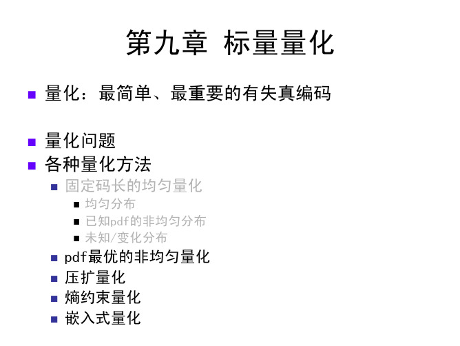
标量量化
与均匀量化器的关系:
当为均匀分布 f X ( x) = c 时, Lloyd-Max量化器变为均 匀量化器 bi bi 1 2 2 (bi − bi −1 ) xf ( x)dx c ∫ xdx ∫ 1 bi −1 bi −1 2 yi = bi = = = (bi + bi −1 ) (bi − bi −1 ) 2 c(bi − bi −1 ) ( ) f x dx ∫
Δk
2 xmax c ( bk ) − c ( bk −1 ) = M
xmax
c ( bk ) c ( bk −1 )
代入上式,得到
2 xmax Δk = Mc′ ( yk )
Δk xmax
非均匀量化器等价于CQ
则高码率下量化误差为
M 1 2 σq = ∑ f X ( yi ) Δ i3 12 i =1
2 q ∞ −∞
D =σ = ∫
( x − Q ( x ) ) f ( x ) dx = ∑ ∫
2 i =1
M
bi
bi −1
( x − yi ) f ( x ) dx
2
Lloyd-Max量化器
亦称为pdf-最佳量化器
D =σ = ∫
2 q
∞
−∞
( x − Q ( x ) ) f ( x ) dx = ∑ ∫ ( x − y ) f ( x ) dx
更多结果…
Laplacian分布的尾巴更长,外侧步长大;同时,内侧步长小,因为在中心附近概率 Pdf最优量化器比pdf最优均匀量化器的SNR高
Lloyd-Max量化器的性质
MeanOutput = Meanintput 1、 2、 VarianceOutput ≤ Varianceintput 3、MSQE:
4_Sampling_Quantization_0809
Department of Electrical and Computer Engineering Faculty of Engineering and ArchitectureAmerican University of BeirutEECE 442L – Communications LaboratoryExperiment onSampling and QuantizationVersion: August 2009Sampling and QuantizationO BJECTIVES•Understand the basic concepts of sampling and quantization.•Demonstrate and analyze the process of sampling with emphasis on the sampling conditions that enable regeneration of an original signal.•Demonstrate and analyze uniform and non-uniform quantization algorithms taking into account the pros and cons of each approach.T HEORETICAL B ACKGROUNDThis experiment gives a theoretical overview as well as a practical insight into the various steps that are needed to convert analog signals (e.g., voice and music), which are predominant in nature, into digital representations.A. I NTRODUCTIONInformation sources can be either analog or discrete in nature. The output of an analog information source can take any value from a continuous range of amplitudes, whereas the output of a discrete information source can take its values from a finite set of amplitudes. Analog information sources can be transformed into digital signals through the processes of sampling and quantization as shown in Figure 1 .B. S AMPLINGThe sampling process transforms a time-continuous signal into a time-discrete signal by extracting samples of the input signal at equidistant time instants. It is important to properly choose the sampling rate so that the obtained sequence of samples uniquely defines the original analog signal. This condition is necessary for perfect reconstruction of the analog signal from the generated set of samples.Sampling and Quantization – August 2009 Page 1Sampling and Quantization – August 2009 Page 2Figure 1: Analog-to-digital conversion process.Assume the analog source signal )(t x is sampled with a rate s s T f /1=,i.e., one sample is obtained every s T seconds. Assume that the signal ()x t is band-limited with no frequency component higher than W . A sampling period of W T s 2/1≤ is sufficient for ideal reconstruction of the signal from its samples. On the other hand, a sampling period W T s 2/1>results in distortion called aliasing that prohibits perfect reconstruction. It is important to note that the case where the sampling rate s f is equal to W 2(or W T s 2/1=) is referred to as the Nyquist sampling rate.In practice, sampling is normally done at a rate higher than the Nyquist sampling rate. This is important to avoids aliasing due to undersampling in case the soure signal is not strictly band-limited. This is also useful for simplifying the design of the reconstruction filter used to recover the original signal from its sampled version at the receiver side. To reconstruct the original signal from its sampled version, a low pass filter is used with high cut off frequency that includes the highest frequency in the source signal.For more background information on sampling, check Section 2.4 in [1] and/or Sections 6.2-6.3 in [2].C. Q UANTIZATIONQuantization is the process of mapping samples of a continuous amplitude waveform into a finite set of amplitudes. The hardware that performs this mapping is normally called the analog-to-digital converter (ADC or A-to-D). Every quantizer is characterized by decision thresholds x k and reconstruction values q k that lie in the center of the quantization-intervalsSampling and Quantization – August 2009 Page 3 [x k , x k+1]. Assuming that there are L quantizing levels and that each quantizing level is represented by an R -bit binary word, it follows that L = 2R . The quantization process is not reversible, and the difference between the input and output of a quantizer is called the quantization error or the quantization noise. Quantizers that exihibit equally spaced increments between possible quantized output levels are called uniform quantizers, otherwise they are called nonuniform quantizers.C.1 U NIFORM Q UANTIZATIONWith uniform quantization, the quantization intervals are all of the same length. The quantization error variance σq 2 of a uniform quantizer can be calculated as follows:22max 2max 223L 231x x R q==−σ where x max is the maximum amplitude of the signal. The signal-to-quantization-noise-ratio of a uniform quantizer can be calculated as follows:⎟⎟⎠⎞⎜⎜⎝⎛=⎟⎟⎠⎞⎜⎜⎝⎛=2221022103log 10log 10)(max x q x U q x L dB SNR σσσ where σx 2 is the variance of the input signal. For the special case where the modulatingsignal is a sinusoid of amplitude A m , its variance is 2/22m x A =σ, and using the number ofbits per sample L R 2log = results in:76.102.623log 10)(210+=⎟⎠⎞⎜⎝⎛=R L dB SNR U q It can be seen that as the number of quantization levels L increases, the value of R increases and, thus, the SNR increases.C.2 O PTIMAL Q UANTIZATIONUniform quantization is the most common method for transforming signals with continuous amplitudes into signals with discrete amplitudes. In general, it is possible to quantize a random variable X with a lower quantization-error variance. This can be achieved by using smaller quantization-intervals where the pdf p X (x) is concentrated. Hence the uantizationSampling and Quantization – August 2009 Page 4 process depends on the input signal. One approach to achieve a lower quantization noise is to perform optimal quantization using the Lloyd-Max algorithm. The variance of the quantization noise to be minimized can be expressed as follows:()()dx x p q x L k X x x k q k k ∑∫=+−=1221σThis is a (2L +1) variable equation (L variables for q and L +1 variables for x ). Minimizing this equation leads to the following results:()[]1,1,,)()()2(,...,3,2,2)1(11+−∈===+=∫∫++k k x Xx x X opt k k k opt k x x X X E dx x p dx x xpq L k q q x k k k kEquation (1) indicates that the optimal decision thresholds for the quantization intervals are the midpoints between two adjacent quantization levels, whereas Equation (2) indicates that the optimal quantization level for a given quantization interval is the expected value of the pdf for that interval.In practice, the above equations can be solved iteratively to obtain the optimal intervals and their corresponding quantization levels. The steps of the algorithm, called Lloyd algorithm, are summarized in Table 1 and further illustrated in Flowchart 1.Table 1: The Lloyd algorithm. Step 1Begin from an arbitrary set of decision thresholds x k (normally uniform thresholds) Step 2Use Equation (2) to get the improved quantization levels q k Step 3Use Equation (1) to get the improved decision thresholds x kStep 4 Compute σq 2. Restart at Step 2 as manytimes as needed to get σq 2 below a givendesired value or until a certain number ofiterations is executedFlowchart 1: The Lloyd algorithm.For more background information on quantization, check Section 6.5 in [1] and/or Section 6.7 in [2].Sampling and Quantization – August 2009 Page 5P REPARATION E XERCISE FOR S AMPLING AND Q UANTIZATIONThis demo gives a primary overview of sampling and quantization for band-limited and non band-limited signals. Open the front panel of “Demo_Sampling_Quantization.vi”, and set the following parameters:Quantity/Setting ValueSignal Type Triangle waveSignal Frequency 2000 HzSampling Frequency4000 HzBits per Sample 3Observe the time domain of the original signal and its sampled version, and their corresponding frequency domain graphs. Inspect also the time domain graphs of the quatized signal for both the original and the sampled signals. In telecommunication systems, quatization is applied after sampling, but for clarification purposes the original quantized signal is included too.Try to think of answers to the following questions: Is the used sampling frequency sufficient to recover the original signal? Increase the number of bits per sample, and observe the quantized graphs. What is the effect of increasing the number of bits per sample? For each signal type in the VI, try to vary the different parameters such as sampling frequency and bits per sample, and analyze the effect of each of these.Sampling and Quantization – August 2009 Page 6Sampling and Quantization – August 2009 Page 7 E XPERIMENT D ESCRIPTIONG ENERAL R ULESIf you open a VI and you are not asked to do any changes to it, then close it withoutsaving changes by clicking on “Defer decision”.Save VIs as [GroupID]_name of VI.viSave plots as [GroupID]_Question number.jpg . For questions with more than one plot,append extra info to the name to differentiate between the plots.P ART I: S AMPLINGIn this part, you will investigate the sampling procedure on various simple input signals. You will consider the effect of aliasing and attempt to correct it by two approaches:(1) increasing the sampling frequency and (2) band-limiting the input signal.A. THE S AMPLING VIOpen the Block Diagram of “SamplingExample.VI ”.The two block subVIs are the following:Sampling.VI Samples a signal according to the specified sampling frequency.SignalReconstruction.VI Reconstructs a sampled signal to its initial state. Q.1 Explain how the case structure between the signal generator and thesampler works. What is its function?Double-click on “Sampling.VI ”.Q.2 Explain in details how sampling is implemented.Double-click on “SignalReconstruction.VI ”.Q.3Explain how reconstruction is performed.B.S AMPLING A S INE W AVEFORMOn the Front Panel of the “SamplingExample.VI”, set the following parameters:Signal Type Sine WaveSignal Frequency 5 kHzPreSampling LPF ON?OFFQ.4 For the given sine wave, what is the theoretical minimum sampling frequency to allow perfect reconstruction? Justify your answer.Q.5 What value would you choose for the Reconstruction LPF Cut-off Frequency? Justify your answer.Set the Sampling Frequency to the value in Q.4, and the Reconstruction LPF Cut-off Frequency to the value in Q.5 and run the VI.Q.6 Do you observe a perfect reconstructed signal? Comment.Run the VI for Sampling Frequencies of 20 kHz, 30 kHz, and 40 kHz.Q.7 Explain the effect of increasing the sampling frequency, and indicate which value would you choose for perfect reconstruction?Q.8 What are the periodic pulses that appear in the spectrum of the sampled signal?Hint: Look at the distance between two consecutive pairs.Set the Sampling Frequency to 7.5 kHz and run the VI.Q.9 What are the extra frequency components that appear in the spectrum of the reconstructed signal? What is this effect called?Sampling and Quantization – August 2009 Page 8C.S AMPLING A S AW-TOOTH W AVEFORMOn the Front Panel of the “SamplingExample.VI”, set the following parameters:Signal Type Sawtooth WaveSignal Frequency 5 kHzPreSampling LPF ON?OFFSampling Frequency 40 kHzReconstruction Cut-off Frequency 5 kHzRun the VI.Q.10 What do you observe on the spectrum graph of the original signal?Inspect the graph of the filtered signal.Q.11 Why is the filtered signal different from the original signal?Hint: Try to vary the value of the Reconstruction Cut-off Frequency. Q.12 How can a pre-sampling filter be used to remove aliasing?Q.13 What is the best value of the Cut-off frequency of the PreSampling LPF when the sampling frequency is 40 kHz? Explain.Set the PreSampling LPF ON and set its Cut-off Frequency to 20 kHz, similarly set the Reconstruction Cut-off Frequency to 20 KHz and run the VI.Q.14 Inspecting the original signal, what is the disadvantage of using a LPF before sampling?Sampling and Quantization – August 2009 Page 9Sampling and Quantization – August 2009 Page 10 P ART II: Q UANTIZATIONIn this part, you will investigate the quantization process including the introduced quantization noise. You will consider two quantization algorithms: (1) uniform quantization and (2) optimal quantization. You will also compare them to each other with regard to quantization SNR.A. T HE Q UANTIZATION VIOpen the Block Diagram of “QuantizeGeneric.VI ”. This VI quantizes input signal samples based on any given set of ordered quantization levels.Q.15 Explain how the quantizer is implemented.Hint: Look in the help at how the “Threshold 1D array” computes the “fractional index”.B. U NIFORM Q UANTIZATIONOpen the Block Diagram of “UniformExample.VI ”.The four block subVIs are the following:GetUniformParameters.VIGets the quantization values k q for a uniform quantizer.QuantizeGeneric.VIAlready seen in part I, it quantizes a signal based on the k q passedfrom the previous GetUniformParameters function.SNR q .VIComputes the quantization SNR in dB.PlotQFunction.VICreates a plot of the quantization staircase function.Q.16 What is the relation between the number of bits per sample and thenumber of quantization levels?Sampling and Quantization – August 2009 Page 11 On the Front Panel of “UniformExample.VI ”, set the following parameters: Signal Frequency 5 kHzBits per Sample3Run the VI.Q.17 What is the resulting value of the SNR in dB? Compare with thetheoretical value. Increase the Bits per Sample to 4 and run the VI.Q.18 Calculate the difference between the resulting value of the SNR withthe value obtained in Q.17. Comment.C. Optimal QuantizationIn this part, you will compare optimal quantization to uniform quantization. The difference is in specifying the quantization steps and their thresholds which are referred to as Parameters in the experiment.Open the “GetCentroid.VI ”. This VI computes the optimal quantization levels over a set of quantization intervals.Q.19 Explain how the VI computes the quantization levels.Open the Block Diagram “UniformVSOptimal.VI ”.The new subVI is:GetOptimalParameters.VI Gets the quantization values k q for an optimal quantizer.On the Front Panel of “UniformVSOptimal.VI ”, set the following parameters: Signal TypeSine Wave Signal Frequency2 kHz Bits per Sample3Examine the waveforms graph to see the difference between the quantized waveforms.Q.20 Why are the first and last quantization intervals smaller for the optimal quantizer compared to the uniform quantizer?Q.21 Note the difference between the two SNR values. Comment.Change the Signal Type to Sinc Function and the Frequency to 5 kHz. Run the VI and note the difference.Q.22 Compare the SNRs of both quantizers. Comment.Q.23 Why is the gap between the optimal and uniform quantizers bigger with Sinc Function compared to Sine Wave?Change the Signal Type to Linear and examine the waveforms and the steps graphs.Q.24 Compare the SNRs of both quantizers. Comment.R EFERENCES[1] J. Proakis and M. Salehi, Communication Systems Engineering. Prentice-Hall, 2ndedition, 2002.[2] S. Haykin, Communication Systems. John Wiley & Sons, 3rd edition, 1994.Sampling and Quantization – August 2009 Page 12。
6_标量量化110309_338405426

量化器输入输出特性曲线表示
yk yk
1. 基本概念
x
x
中平型均匀量化器
中升型均匀量化器
yk
yk
x
x
中平型非均匀量化器
中升型非均匀量化器
图2. 几种量化器输入输出特性
量化误差(量化噪声)
q = x − y = x − Q (x)
对于确定信号 x,q 也是确定信号; 对于语音、图象等随机信号,q 也是随机信号。
B
2.均匀量化
各量化区间相等 :
∆ k = xk +1 − xk = ∆
设量化器量化范围是从 –V 到 +V,则
k = 1,2, L , L
∆=
量化电平取各量化区间中点:
2V 2V = R L 2
yk =
x k +1 + x k 2
6
(1) 输入信号幅度受限, x ≤ V
量化误差: • 量化误差范围:
1. 基本概念
设 x 的概率分布密度函数是 px (x),q 的概率分布密度为 pq(q),,则 q 的均方值为:
σ
2 q
= E q
[ ]= ∫
2
∞
−∞
q 2 p q ( q ) dq
由于 q=x-Q(x) 是 x 的函数,所以量化误差功率
σ = E [q ] = ∫
2 q 2
L 2 q xk +1
π
V2 = 2 2 − 2 R = 1 .5 × 2 2 R V 2 3
db max
• •
SNR
= 6 . 02 R + 1 . 76
语音为非平稳随机信号,电话语音电平变化超过 40db。对小信号电平 输入,SNR应保证约 20~30db,即最大 SNR需 60~70db,均匀量化 器要11~13比特。
Lloyd-MAX算法的研究报告
Lloyd —Max 算法的总结摘 要:本文分析模拟—数字信号转变过程中抽象信号为离散时间,幅度连续,无记忆的 随机信号的最佳量化问题。
并对算法做了总结,应用MATLAB 编写程序实现该算 法,最后给出了运用该程序进行计算的几个例子。
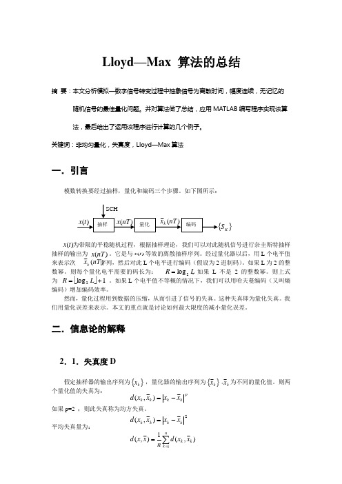
关键词:非均匀量化,失真度,Lloyd —Max 算法一.引言模数转换要经过抽样,量化和编码三个步骤。
如下图所示:为带限的平稳随机过程,根据抽样理论,我们可以对此随机信号进行奈圭斯特抽样抽样的输出为 。
它是与 等效的离散抽样序列。
经过量化器以后,用L 个电平值来表示次 序列,然后对此L 个电平进行编码(假设为2进制码)。
如果L 为2的整数幂。
则每个量化电平需要的码长为: , 如果L 不是2的整数幂。
则上式为 。
如果L 个电平值不等概的情况下,我们可以用哈夫蔓编码(又叫熵编码)增加编码效率。
然而,量化过程用到数据的压缩,从而引进了信号的失真。
这种失真即为量化失真。
我们用量化误差来表示。
本文的重点就是讨论如何最大限度的减小量化误差。
二.信息论的解释2.1.失真度D假定抽样器的输出序列为 ,量化器的输出序列为 。
为不同的量化值。
则两个量化值的失真为:如果p=2 ;则此失真称为均方失真。
平均失真量为:p k k k k x x x x d ~)~,(-=∑==n k k k x xd n x x d 1)~,(1)~,(2~)~,(k k k k x x x x d -=}K S )(t x )(nT x )(t x )(~nT x k L R 2log =⎣⎦1log 2+=L R {}k x ~{}k x kx ~如果x (t )是服从概率密度函数为p (x )的随机信号,则:失真度D :如果用: 来表示。
量化噪声MSE : 量化信噪比SNR : 2.2.率失真函数R (D ):我们假定信源为无记忆,连续幅度,它的幅度概率密度函数为p (x ),则率失真函数R (D )的表示式为:现在分析一下失真函数R (D )的意义。
精品文档-数字图像处理(第三版)(何东健)-第9章
第9章 图像编码
它将标量数据组织成一系列k维矢量, 根据一定的失真测 度(如均方误差、 lp范数、 极大范数等)在码书中搜索出 与输入矢量失真最小的码字的索引, 传输时仅传输相应码字 的索引,接收方根据码字索引在码书中查找对应码字, 再现 输入矢量。 矢量量化编码的核心是码书设计, 经典的码书设 计算法有LBG(Linde, Buzo和Gray三人的首字母) 算法(又称为K-means算法)。 码书设计过程就是寻求把M 个训练矢量分成N类(N<M)的一种最佳方案(如均方误差最 小), 并把各类的中心矢量作为码书中的码字。
第9章 图像编码 9.1.2
人们不断提出新的图像编码方法, 如基于人工神经网络 的编码、 子带编码(Sub band Coding)、 分形编码 (Fractal Coding)、 小波编码(Wavelet Coding)、 基 于模型的编码(Model based Coding)、 基于对象的编码 (Object based Coding)和基于语义的编码(Semantic Based Coding)等。
(2) 预测编码。 预测编码是基于图像数据的空间或时 间冗余特性, 它用相邻的已知像素(或像素块)来预测当 前像素(或像素块)的取值, 然后再对预测误差进行量化和 编码。 预测编码可分为帧内预测和帧间预测, 常用的预测编 码有差分脉码调制(DPCM, Differential Pulse Code Modulation)和运动补偿法。 图9-1和图9-2分别给出了无损 预测编码和有损预测编码系统的原理图,均包括编码器和解码 器, 其中符号编码器通常采用变长编码。
第9章 图像编码 信息熵是无损编码的理论极限, 当平均码长大于等于信 息熵时, 总可设计出一种无失真编码, 这是熵编码的理论基 础。 若使用相同长度的码字表示信源符号, 则称该编码方法 为等长编码, 否则称为变长编码。 变长编码的基本原理是给 出现概率较大的符号赋予短码字, 而给出现概率较小的符号 赋予长码字, 从而使得最终的平均码长很小。 哈夫曼编码和 香农-范诺编码就是两种变长编码方法。
DPCM_编码解码
}
}
conStructArray数组里面存放的。考虑到第0行,第0列,作为最初的预测参考依据,这两行原值编码,以保证预测的准确性。最后一列由于位置原因也进行原值编码。对于预测误差,首先放大100倍进行判决,量化以后又缩小100倍,与预测值求和,这样保证了精度。
/*由前面知道,判决电平数组和量化重建数组中的数据都扩大了100倍,因此将预测误差nErr扩大100倍,进行判决*/
nErr=(nR-nPre)*100;
int k;
for (k=0;k<3;k++)
{
if (nErr<z_level_two[k])break;
}
/*得到重建值,用于后面的像素的预测,q_level_two[k]/100是由于上面q_level_two中的数据扩大了100倍*/
将上面转化以后的判决电平和量化重建电平存储到数组中例如2bitpixel情况下的判决电平和量化重建电平分别用以下两个数组存储为了进行整数运算尽量避免存储运算同时保留应有精度我将表中数据扩大100后取整因此数组初始化如下
帧内DPCM编码
一、实现要求
DPCM编码解码的流程图如下图
具体要求如下
1、线性预测器
2、DPCM的代码实现(代码在VS2010中调试通过)
这里2bit/pixel情况为例,其他类似。
1)将上面转化以后的判决电平和量化重建电平存储到数组中
例如2bit/pixel情况下的判决电平和量化重建电平分别用以下两个数组存储,为了进行整数运算尽量避免存储运算,同时保留应有精度,我将表中数据扩大100倍以后取整,因此数组初始化如下:
if (i==0||j==0||j==PIC_WIDTH-1)
完全背包问题实验报告
一、实验背景完全背包问题(Full Knapsack Problem)是组合优化领域中的一个经典问题。
它指的是给定n种物品,每种物品的数量无限,每种物品的重量和价值已知,求出装满一个容量为W的背包所需的最小价值。
完全背包问题具有广泛的应用背景,如货物装载、资源分配、网络路由等。
二、实验目的1. 理解完全背包问题的基本概念和求解方法。
2. 掌握动态规划算法在解决完全背包问题中的应用。
3. 分析不同算法的时间复杂度和空间复杂度,为实际应用提供参考。
三、实验环境1. 操作系统:Windows 102. 编程语言:Python3.83. 开发工具:PyCharm四、实验方法1. 动态规划法动态规划法是解决完全背包问题的常用方法。
其基本思想是将问题分解为子问题,并存储子问题的解以避免重复计算。
(1)定义状态设dp[i][j]表示前i种物品装满容量为j的背包的最大价值。
(2)状态转移方程dp[i][j] = max(dp[i-1][j], dp[i-1][j-w[i]] + v[i]),其中i表示物品数量,j表示背包容量,w[i]表示第i种物品的重量,v[i]表示第i种物品的价值。
(3)初始化dp[0][j] = 0,表示没有物品时,无论背包容量为多少,价值都为0。
(4)遍历按照物品数量i从1到n,背包容量j从1到W进行遍历,根据状态转移方程计算dp[i][j]。
(5)输出结果dp[n][W]即为装满容量为W的背包所需的最小价值。
2. 分支限界法分支限界法是一种搜索算法,通过剪枝来降低搜索空间,从而提高求解效率。
(1)定义状态设Node为节点类,表示背包问题的状态。
Node包含以下属性:当前物品数量、当前背包容量、当前背包价值、当前解。
(2)构建搜索树以物品数量为分支,从根节点开始递归构建搜索树。
对于每个节点,根据当前背包容量和物品重量,判断是否继续向下搜索。
(3)剪枝对于每个节点,如果当前背包价值已经超过已知的最大价值,则剪枝,不再向下搜索。
欧式距离聚类算法
欧式距离聚类算法欧式距离聚类算法(Euclidean distance clustering algorithm)是一种基于距离的聚类算法,也称为K-means算法或Lloyd's算法。
该算法根据数据点之间的欧氏距离来划分数据点,并将相似的数据点分配到同一簇中。
本文将介绍欧式距离聚类算法的原理、步骤和实现方法。
欧式距离(Euclidean distance)是指在欧几里得空间中两个点之间的直线距离。
在二维空间中,欧式距离可以表示为:d = √((x2 - x1)^2 + (y2 - y1)^2)其中,(x1, y1)和(x2, y2)是两个数据点的坐标。
在高维空间中,欧式距离的计算方式类似。
欧式距离聚类算法的基本步骤如下:1. 初始化:选择聚类的簇数K,并随机选择K个数据点作为初始聚类中心。
2. 分配数据点:计算每个数据点到每个聚类中心的欧氏距离,并将数据点分配到距离最近的聚类中心所对应的簇中。
3. 更新聚类中心:对于每个簇,计算该簇中所有数据点的均值,将均值作为新的聚类中心。
4. 重复步骤2和步骤3,直到聚类中心不再变化或达到预设的迭代次数。
在实现欧式距离聚类算法时,可以使用以下伪代码作为参考:```pythondef euclidean_distance(p1, p2):# 计算两个数据点之间的欧式距离return sqrt(sum((x - y) ** 2 for x, y in zip(p1, p2)))def kmeans(data, k, max_iter):# 初始化聚类中心centers = random.sample(data, k)old_centers = None# 迭代for _ in range(max_iter):# 分配数据点到最近的聚类中心clusters = [[] for _ in range(k)]for point in data:distances = [euclidean_distance(point, center) for center in centers]cluster_index = distances.index(min(distances))clusters[cluster_index].append(point)# 更新聚类中心old_centers = centerscenters = [np.mean(cluster, axis=0) for cluster in clusters]# 判断是否收敛if np.array_equal(old_centers, centers):breakreturn clusters```该伪代码简要描述了欧式距离聚类算法的实现过程。
- 1、下载文档前请自行甄别文档内容的完整性,平台不提供额外的编辑、内容补充、找答案等附加服务。
- 2、"仅部分预览"的文档,不可在线预览部分如存在完整性等问题,可反馈申请退款(可完整预览的文档不适用该条件!)。
- 3、如文档侵犯您的权益,请联系客服反馈,我们会尽快为您处理(人工客服工作时间:9:00-18:30)。
Lloyd —Max 算法的总结摘 要:本文分析模拟—数字信号转变过程中抽象信号为离散时间,幅度连续,无记忆的 随机信号的最佳量化问题。
并对算法做了总结,应用MATLAB 编写程序实现该算 法,最后给出了运用该程序进行计算的几个例子。
关键词:非均匀量化,失真度,Lloyd —Max 算法一.引言模数转换要经过抽样,量化和编码三个步骤。
如下图所示:为带限的平稳随机过程,根据抽样理论,我们可以对此随机信号进行奈圭斯特抽样抽样的输出为 。
它是与 等效的离散抽样序列。
经过量化器以后,用L 个电平值来表示次 序列,然后对此L 个电平进行编码(假设为2进制码)。
如果L 为2的整数幂。
则每个量化电平需要的码长为: , 如果L 不是2的整数幂。
则上式为 。
如果L 个电平值不等概的情况下,我们可以用哈夫蔓编码(又叫熵编码)增加编码效率。
然而,量化过程用到数据的压缩,从而引进了信号的失真。
这种失真即为量化失真。
我们用量化误差来表示。
本文的重点就是讨论如何最大限度的减小量化误差。
二.信息论的解释2.1.失真度D假定抽样器的输出序列为 ,量化器的输出序列为 。
为不同的量化值。
则两个量化值的失真为:如果p=2 ;则此失真称为均方失真。
平均失真量为:p k k k k x x x x d ~)~,(-=∑==n k k k x xd n x x d 1)~,(1)~,(2~)~,(k k k k x x x x d -=}K S )(t x )(nT x )(t x )(~nT x k L R 2log =⎣⎦1log 2+=L R {}k x ~{}k x kx ~如果x (t )是服从概率密度函数为p (x )的随机信号,则:失真度D :如果用: 来表示。
量化噪声MSE : 量化信噪比SNR : 2.2.率失真函数R (D ):我们假定信源为无记忆,连续幅度,它的幅度概率密度函数为p (x ),则率失真函数R (D )的表示式为:现在分析一下失真函数R (D )的意义。
给定允许的失真度D 的情况下,寻求平均互 信息量的最小值。
在信源编码过程中,该最小值的意义即为:给定一定的失真度D ,存在最小的编码码长R 。
即可寻求最小的量化电平数L 。
因此,进行最佳量化设计的目标可以看成以下问题: A :给定量化电平数L ,寻求一种方法使得失真度D 最小。
B :对于允许的失真度D ,怎样减少量化电平数L 。
本文章将讨论问题A ,即怎样寻择量化方法使D 最小。
量化的方法有很多,如权量化,自适应量化,矢量量化和标量量化。
下面将对标量量化进行讨论。
三.标量量化的最佳量化问题在信源量化中,如果我们知道量化器的输入信号为概率密度函数为p (x ),则量化器可以进行优化。
同样的,设输入的信号概率密度函数为p (x ),量化电平数设为L 。
误差函数设为量化失真度为D 。
最佳量化器的目的即为减小D ,为此,必须正确选取最佳量化电平值和量化区间 。
Lloyd-Max 算法就是最佳量化的好的实现方法。
我们称用Lloyd-Max 算法的量化器为Lloyd-Max 最佳量化器。
为讨论该算法,我们先介绍均匀量化对于均匀量化,设量化电平为: ,其中,Δ为量化台阶 当(k-1)Δ≤x<k Δ时,量化为 假设均匀量化器的输出为对称的偶数个电平,则平均失真为:{}⎰+∞∞-==dx x p x x d x x d E D n n )()~,(~,( ∑⎰∑⎰==---==L k x x L k x x k k k k k k dxx p x x dx x p x x d 11211)()~()()~,(n x x x f ~~)(+==()D n E MSE ==2~())~(22n E x E SNR ={}[])~,()(~,(~x x I MIN D R Dx x d E x x P ≤=∆-=)12(21~k x k k x ~∑⎰-=∆∆-+-∆-=121)1()())12(21(2L k K K dx x p x k f D )~,(x x d对Δ求导,即可得到最小的量化失真D。
对上式求导为:给定一个p (x ),可以通过计算机编程设计得到最佳量化的矢量步长 。
Max 首先对输入信号为均值为0,单位方差的高斯信号进行了计算。
四.Lloyd —Max 算法对于输入信号分布函数p (x ),量化输出电平 ,量化电平数为L,量化区间端点值为当 时 则量化为 . ,. 则失真度为:对 和 进行优化以减小D ,同时对 和 分别求导,得到下面两个等式: 采用均方误差则 ,所以可以得出:这两个式子可以通过计算机编程进行连续的迭代计算,求出最佳的 和 ,以尽可能达到最小的D 。
五.MATALB 的编程实现给定量化电平L 和输入信号概率密度函数p (x )和信号可能的最大值,最小值进行迭代,求出最佳量化电平 和量化范围 。
并给出了一个结果。
其中的失真度D 的绝对值过大,仅仅是为了说明情况,具体的计算可以根据需要的值进行设置两次迭带中的D 值之差,进而计算出比较精确的结果。
(程序清单和计算结果见附录)∑⎰-=∆∆-+-∆-'-121)1()())12(21()12(L k K K dx x p x k f k 0)())12(21()1()12(=-∆-'-⎰∞∆-L dx x p x k f L ⎰∞∆--∆-)12()())12(21(2L dx x p x k f {}k x ~{}k x {}k k x x x 〈≤-1{}k x ~-∞=0x +∞=L x ∑⎰=--=L k x x k k k dx x p x x f D 11)()~({}k x ~{}k x {}k x~{}k x 13,2,1)~()~(1-=-=-+L k x x f x x f k k k k L k dx x p x x f k k x x k k 3,2,10)()~(1==-'⎰-2)(x x f =13,2,1~~(21)1-=+=+L k x x x k k k L k dx x p x x k k x x k k 3,2,10)()~(12==-⎰-L k dx x p dx x xp x k k k k x x x x k 3,2,1)()(11==⎰⎰--{}k x~{}k x {}k x~{}k x六.结束语Lloyd—Max算法的特点是:量化电平集中在信号概率大的区域。
在量化电平极小的情况下,均匀量化和非均匀量化的性能差不多。
但是随着量化电平数的增加,非均匀量化产生的失真度明显比均匀量化小。
根据信号的概率密度函数进行量化,将时间离散,幅度连续的信号量化到各个离散的电平上,它们对应了相应的概率。
可以据此进行熵编码,以期在相同的失真度条件下得到最小的码长R。
非均匀量化简单有效的实现且应用在商业电话的对数量化器,根据人的语音特点,在低幅度时用比较多的量化电平(量化台阶小),而在信号不常发生的大幅度电平值时,量化电μ律压缩和欧洲的A-律压缩。
平就大,常用的技术有美国的-参考文献:[1]:John..G.Proakis Digital Communication,电子工业出版社影印版[2]:Theodore.S.Rappaport Wireless communication , 电子工业出版社影印版[3]:傅祖芸信息论基础,电子工业出版社[4]:沈振元,聂志泉,区雪荷通信系统原理西安电子科技大学出版社附录:源程序清单:1:MAINfunction mainclear all;string1=input('Please input the pdf of the signal: ');string2=string1;disp('Please input the max amplitude of the signal:');xmax=input(' ');disp('Please input the min amplitude of the signal:');xmin=input(' ');disp('Please input the number of the quantization levels:'); qsteps=input(' ');lloyedmax(string2,xmax,xmin,qsteps)2:Lloyd—Maxfunction d=lloyedmax(pdf,xmax,xmin,qsteps)g=inline(pdf);step=abs((xmax-xmin))/qsteps;for i=1:qstepsxvalue(i)=xmin+(i-0.5)*step;end;dold=1;dsum=0;j=0;while abs(dold-dsum)>0.01j=j+1;x(j)=dsum;dold=dsum;xdomin(1)=xmin;xdomin(qsteps+1)=xmax;for i=2:qstepsxdomin(i)=(xvalue(i-1)+xvalue(i))./2;enddsum=0;for i=2:qsteps+1xstemp=xdomin(i-1):abs(xdomin(i)-xdomin(i-1))/100:xdomin(i); y=((xvalue(i-1)-xstemp).^2).*g(xstemp);d=trapz(xstemp,y);dsum=dsum+d;endfor i=2:qsteps+1xstemp=xdomin(i-1):abs(xdomin(i)-xdomin(i-1))/100:xdomin(i); y1=xstemp.*g(xstemp);y2=g(xstemp);d1=trapz(xstemp,y1);d2=trapz(xstemp,y2);xvalue(i-1)=d1/d2;figure(j);plot(xvalue,1:1:qsteps,'*',xdomin,1:1:qsteps+1,'x')ylabel('the compute numbers')xlabel('regions (x) and outputlevels (*)')endoutputlevel=xvalueregions=xdomindistortion=dsumendj=j+1;x(j)=dsumoutputlevel=xvalueregions==xdominfigure(j);ylabel('the compute numbers')xlabel('regions (x) and outputlevels (*)')plot(xvalue,1:1:qsteps,'*',xdomin,1:1:qsteps+1,'x')figure(j+1)clear c;for i=2:jc(i-1)=x(i);endplot(1:1:j-1,c,'*')xlabel('the compute numbers')ylabel('everyone distortion')附录:计算举例:例子: 1.当 时,量化电平数L=16; =2。