Lecture2
lecture 2--听辨

听力训练 VS 听辨过程 1
英语听力训练中比 较注重语言层面, 即十分注意语音、 语调和语言的表达 及用法。
译员在听辨过程中 所注重的是意思, 或是讲话者的意图 而不是具体的词句 表达。所以译员在 听到一段话之后在 头脑中形成的是一 个有逻辑关系的语 意整体,而不仅仅 是词句的简单集合。
听力训练 VS 听辨过程 2
• 对照关系:like, similarly, in a similar manner, likewise • 对比关系:different from, unlike, by contrast, on the other hand, on the contrary, • conversely
• 解释关系: that is to say, in other words, this means
先后次序:first of all, next, before, after, previously, simultaneously, eventually, finally
Bugs in LCII 恼人的听辨“虫”
1. unknown words 生词 2. culturally-burdened phrases or idioms 英语中 的文化陷阱(容易望文生义) 3. illogical flow of thought逻辑混乱 4. heavy accent 口音浓重 5. unfamiliar topic 不了解主题知识 6. too quick a delivery speed 语速过快 7. blurred point of view 意思不明确 8.数字
逻辑关系和对应的标示词
并列关系:and, too, at the same time, meanwhile, in the meantime, as well • • • • • 递进关系:also, moreover, in addition, furthermore, besides, not only, on top of that, apart from 转折关系:but, however, though, whereas, nevertheless, in fact, instead 让步关系:in spite of, despite, although, even though 因果关系:so, thus, hence, as a result, consequently, reason, because, for, due to, accordingly
Lecture2我们的身体——人体的科学教案

Lecture2 我们的身体——人体的科学(教案)一.教学目标1.知识性目标:大致了解身体结构;了解基本器官以及消化系统、呼吸系统的工作原理。
2.感受人体构造的“神奇”,培养探索性的好奇心。
3.介绍一些日常生活中自我保护和救助的小知识。
4.培养爱护身体的意识。
二.准备:1.课前在黑板上画人体结构图。
2.网球+网兜(模拟肺泡的结构)3.咀嚼、吞咽、消化、呼吸等的音效[注:六年级的教室里墙上有几个插座,事先不知,所以未带音箱去。
如果知道可以和mp3结合使用。
]三.教学设计Part I 引入:了解身体的意义我们今天要讲的话题是我们的身体。
可能有人觉得,这个话题太普通了,我们对自己的身体还不熟悉吗!是啊,我们每天每时每刻都在用自己的身体,可是我们真的很了解它吗?[跟着几个简单问题后,问:你有几颗牙齿?——资料:乳牙20颗,7-25换牙后(每换一颗牙需要半年)在乳牙后还会长出12 只恒磨牙,共32 颗,但有的人最后四颗磨牙终生不萌出或部份萌出。
全口牙齿总咬力男子为1408公斤,女子为936公斤;但如果失掉一颗牙齿,总咬力会减少200多公斤,缺二颗牙齿,总咬力减少50%-剩一半-牙齿需要配合才能最好地发挥作用,每一颗牙齿都要保护。
]其实这只是一个简单的例子,我们的身体中的奥秘还多着呢。
解答这些奥秘,有时候仅仅是为了满足我们的好奇心,但是另外有些时候是因为这些奥秘的答案实在太重要了,让人们不能忽视它。
比如,医生只有知道人体是怎么构造的,有哪些器官,这些器官在哪儿,都是怎么工作的,才能有效地诊断、治疗病人。
但是,在很长时间的一段时间里,医生连人体主要器官的位置都搞不清楚,因为当时解剖尸体是被禁止的(谁也不敢把人体“切开来”看看里面究竟是什么样)。
西方1800多年前有一位医学家叫盖仑,他认为解剖学对医生来说就像设计图纸对建筑师一样重要。
但是因为没法解剖人体,他只能解剖动物,比如猴子、猪、山羊、河马,然后从这些动物的结构上来猜测人体的结构。
lecture_2(博弈论讲义GameTheory(MIT))
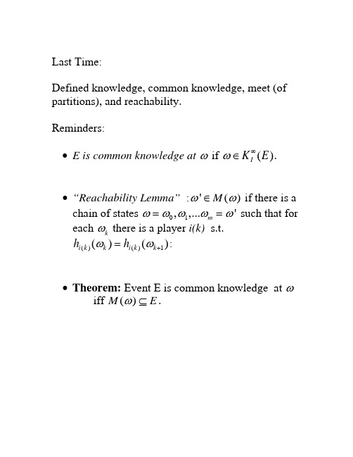
Last Time:Defined knowledge, common knowledge, meet (of partitions), and reachability.Reminders:• E is common knowledge at ω if ()I K E ω∞∈.• “Reachability Lemma” :'()M ωω∈ if there is a chain of states 01,,...m 'ωωωωω== such that for each k ω there is a player i(k) s.t. ()()1()(i k k i k k h h )ωω+=:• Theorem: Event E is common knowledge at ωiff ()M E ω⊆.How does set of NE change with information structure?Suppose there is a finite number of payoff matrices 1,...,L u u for finite strategy sets 1,...,I S SState space Ω, common prior p, partitions , and a map i H λso that payoff functions in state ω are ()(.)u λω; the strategy spaces are maps from into . i H i SWhen the state space is finite, this is a finite game, and we know that NE is u.h.c. and generically l.h.c. in p. In particular, it will be l.h.c. at strict NE.The “coordinated attack” game8,810,11,100,0A B A B-- 0,010,11,108,8A B A B--a ub uΩ= 0,1,2,….In state 0: payoff functions are given by matrix ; bu In all other states payoff functions are given by . a upartitions of Ω1H : (0), (1,2), (3,4),… (2n-1,2n)... 2H (0,1),(2,3). ..(2n,2n+1)…Prior p : p(0)=2/3, p(k)= for k>0 and 1(1)/3k e e --(0,1)ε∈.Interpretation: coordinated attack/email:Player 1 observes Nature’s choice of payoff matrix, sends a message to player 2.Sending messages isn’t a strategic decision, it’s hard-coded.Suppose state is n=2k >0. Then 1 knows the payoffs, knows 2 knows them. Moreover 2 knows that 1knows that 2 knows, and so on up to strings of length k: . 1(0n I n K n -Î>)But there is no state at which n>0 is c.k. (to see this, use reachability…).When it is c.k. that payoff are given by , (A,A) is a NE. But.. auClaim: the only NE is “play B at every information set.”.Proof: player 1 plays B in state 0 (payoff matrix ) since it strictly dominates A. b uLet , and note that .(0|(0,1))q p =1/2q >Now consider player 2 at information set (0,1).Since player 1 plays B in state 0, and the lowest payoff 2 can get to B in state 1 is 0, player 2’s expected payoff to B at (0,1) is at least 8. qPlaying A gives at most 108(1)q q −+−, and since , playing B is better. 1/2q >Now look at player 1 at 1(1,2)h =. Let q'=p(1|1,2), and note that '1(1)q /2εεεε=>+−.Since 2 plays B in state 1, player 1's payoff to B is at least 8q';1’s payoff to A is at most -10q'+8(1-q) so 1 plays B Now iterate..Conclude that the unique NE is always B- there is no NE in which at some state the outcome is (A,A).But (A,A ) is a strict NE of the payoff matrix . a u And at large n, there is mutual knowledge of the payoffs to high order- 1 knows that 2 knows that …. n/2 times. So “mutual knowledge to large n” has different NE than c.k.Also, consider "expanded games" with state space . 0,1,....,...n Ω=∞For each small positive ε let the distribution p ε be as above: 1(0)2/3,()(1)/3n p p n ee e e -==- for 0 and n <<∞()0p ε∞=.Define distribution by *p *(0)2/3p =,. *()1/3p ∞=As 0ε→, probability mass moves to higher n, andthere is a sense in which is the limit of the *p p εas 0ε→.But if we do say that *p p ε→ we have a failure of lower hemi continuity at a strict NE.So maybe we don’t want to say *p p ε→, and we don’t want to use mutual knowledge to large n as a notion of almost common knowledge.So the questions:• When should we say that one information structure is close to another?• What should we mean by "almost common knowledge"?This last question is related because we would like to say that an information structure where a set of events E is common knowledge is close to another information structure where these events are almost common knowledge.Monderer-Samet: Player i r-believes E at ω if (|())i p E h r ω≥.()r i B E is the set of all ω where player i r- believesE; this is also denoted 1.()ri B ENow do an iterative definition in the style of c.k.: 11()()rr I i i B E B E =Ç (everyone r-believes E) 1(){|(()|())}n r n ri i I B E p B E h r w w -=³ ()()n r n rI i i B E B =ÇEE is common r belief at ω if ()rI B E w ¥ÎAs with c.k., common r-belief can be characterized in terms of public events:• An event is a common r-truism if everyone r -believes it when it occurs.• An event is common r -belief at ω if it is implied by a common r-truism at ω.Now we have one version of "almost ck" : An event is almost ck if it is common r-belief for r near 1.MS show that if two player’s posteriors are common r-belief, they differ by at most 2(1-r): so Aumann's result is robust to almost ck, and holds in the limit.MS also that a strict NE of a game with knownpayoffs is still a NE when payoffs are "almost ck” - a form of lower hemi continuity.More formally:As before consider a family of games with fixed finite action spaces i A for each player i. a set of payoff matrices ,:l I u A R ->a state space W , that is now either finite or countably infinite, a prior p, a map such that :1,,,L l W®payoffs at ω are . ()(,)()w u a u a l w =Payoffs are common r-belief at ω if the event {|()}w l w l = is common r belief at ω.For each λ let λσ be a NE for common- knowledgepayoffs u .lDefine s * by *(())s l w w s =.This assigns each w a NE for the corresponding payoffs.In the email game, one such *s is . **(0)(,),()(,)s B B s n A A n ==0∀>If payoffs are c.k. at each ω, then s* is a NE of overall game G. (discuss)Theorem: Monder-Samet 1989Suppose that for each l , l s is a strict equilibrium for payoffs u λ.Then for any there is 0e >1r < and 1q < such that for all [,1]r r Î and [,1]q q Î,if there is probability q that payoffs are common r- belief, then there is a NE s of G with *(|()())1p s s ωωω=>ε−.Note that the conclusion of the theorem is false in the email game:there is no NE with an appreciable probability of playing A, even though (A,A) is a strict NE of the payoffs in every state but state 0.This is an indirect way of showing that the payoffs are never ACK in the email game.Now many payoff matrices don’t have strictequilibria, and this theorem doesn’t tell us anything about them.But can extend it to show that if for each state ω, *(s )ω is a Nash (but not necessarily strict Nash) equilibrium, then for any there is 0e >1r < and 1q < such that for all [,1]r r Î and [,1]q q Î, if payoffs are common r-belief with probability q, there is an “interim ε equilibria” of G where s * is played with probability 1ε−.Interim ε-equilibria:At each information set, the actions played are within epsilon of maxing expected payoff(((),())|())((',())|())i i i i i i i i E u s s h w E u s s h w w w w e-->=-Note that this implies the earlier result when *s specifies strict equilibria.Outline of proof:At states where some payoff function is common r-belief, specify that players follow s *. The key is that at these states, each player i r-believes that all other players r-believe the payoffs are common r-belief, so each expects the others to play according to s *.*ΩRegardless of play in the other states, playing this way is a best response, where k is a constant that depends on the set of possible payoff functions.4(1)k −rTo define play at states in */ΩΩconsider an artificial game where players are constrained to play s * in - and pick a NE of this game.*ΩThe overall strategy profile is an interim ε-equilibrium that plays like *s with probability q.To see the role of the infinite state space, consider the"truncated email game"player 2 does not respond after receiving n messages, so there are only 2n states.When 2n occurs: 2 knows it occurs.That is, . {}2(0,1),...(22,21,)(2)H n n =−−n n {}1(0),(1,2),...(21,2)H n =−.()2|(21,2)1p n n n ε−=−, so 2n is a "1-ε truism," and thus it is common 1-ε belief when it occurs.So there is an exact equilibrium where players playA in state 2n.More generally: on a finite state space, if the probability of an event is close to 1, then there is high probability that it is common r belief for r near 1.Not true on infinite state spaces…Lipman, “Finite order implications of the common prior assumption.”His point: there basically aren’t any!All of the "bite" of the CPA is in the tails.Set up: parameter Q that people "care about" States s S ∈,:f S →Θ specifies what the payoffs are at state s. Partitions of S, priors .i H i pPlayer i’s first order beliefs at s: the conditional distribution on Q given s.For B ⊆Θ,1()()i s B d =('|(')|())i i p s f s B h s ÎPlayer i’s second order beliefs: beliefs about Q and other players’ first order beliefs.()21()(){'|(('),('))}|()i i j i s B p s f s s B h d d =Îs and so on.The main point can be seen in his exampleTwo possible values of an unknown parameter r .1q q = o 2qStart with a model w/o common prior, relate it to a model with common prior.Starting model has only two states 12{,}S s s =. Each player has the trivial partition- ie no info beyond the prior.1122()()2/3p s p s ==.example: Player 1 owns an asset whose value is 1 at 1θ and 2 at 2θ; ()i i f s θ=.At each state, 1's expected value of the asset 4/3, 2's is 5/3, so it’s common knowledge that there are gains from trade.Lipman shows we can match the players’ beliefs, beliefs about beliefs, etc. to arbitrarily high order in a common prior model.Fix an integer N. construct the Nth model as followsState space'S ={1,...2}N S ´Common prior is that all states equally likely.The value of θ at (s,k) is determined by the s- component.Now we specify the partitions of each player in such a way that the beliefs, beliefs about beliefs, look like the simple model w/o common prior.1's partition: events112{(,1),(,2),(,1)}...s s s 112{(,21),(,2),(,)}s k s k s k -for k up to ; the “left-over” 12N -2s states go into 122{(,21),...(,2)}N N s s -+.At every event but the last one, 1 thinks the probability of is 2/3.1qThe partition for player 2 is similar but reversed: 221{(,21),(,2),(,)}s k s k s k - for k up to . 12N -And at all info sets but one, player 2 thinks the prob. of is 1/3.1qNow we look at beliefs at the state 1(,1)s .We matched the first-order beliefs (beliefs about θ) by construction)Now look at player 1's second-order beliefs.1 thinks there are 3 possible states 1(,1)s , 1(,2)s , 2(,1)s .At 1(,1)s , player 2 knows {1(,1)s ,2(,1)s ,(,}. 22)s At 1(,2)s , 2 knows . 122{(,2),(,3),(,4)}s s s At 2(,1)s , 2 knows {1(,2)s , 2(,1)s ,(,}. 22)sThe support of 1's second-order beliefs at 1(,1)s is the set of 2's beliefs at these info sets.And at each of them 2's beliefs are (1/3 1θ, 2/3 2θ). Same argument works up to N:The point is that the N-state models are "like" the original one in that beliefs at some states are the same as beliefs in the original model to high but finite order.(Beliefs at other states are very different- namely atθ or 2 is sure the states where 1 is sure that state is2θ.)it’s1Conclusion: if we assume that beliefs at a given state are generated by updating from a common prior, this doesn’t pin down their finite order behavior. So the main force of the CPA is on the entire infinite hierarchy of beliefs.Lipman goes on from this to make a point that is correct but potentially misleading: he says that "almost all" priors are close to a common. I think its misleading because here he uses the product topology on the set of hierarchies of beliefs- a.k.a topology of pointwise convergence.And two types that are close in this product topology can have very different behavior in a NE- so in a sense NE is not continuous in this topology.The email game is a counterexample. “Product Belief Convergence”:A sequence of types converges to if thesequence converges pointwise. That is, if for each k,, in t *i t ,,i i k n k *δδ→.Now consider the expanded version of the email game, where we added the state ∞.Let be the hierarchy of beliefs of player 1 when he has sent n messages, and let be the hierarchy atthe point ∞, where it is common knowledge that the payoff matrix is .in t ,*i t a uClaim: the sequence converges pointwise to . in t ,*i t Proof: At , i’s zero-order beliefs assignprobability 1 to , his first-order beliefs assignprobability 1 to ( and j knows it is ) and so onup to level n-1. Hence as n goes to infinity, thehierarchy of beliefs converges pointwise to common knowledge of .in t a u a u a u a uIn other words, if the number of levels of mutual knowledge go to infinity, then beliefs converge to common knowledge in the product topology. But we know that mutual knowledge to high order is not the same as almost common knowledge, and types that are close in the product topology can play very differently in Nash equilibrium.Put differently, the product topology on countably infinite sequences is insensitive to the tail of the sequence, but we know that the tail of the belief hierarchy can matter.Next : B-D JET 93 "Hierarchies of belief and Common Knowledge”.Here the hierarchies of belief are motivated by Harsanyi's idea of modelling incomplete information as imperfect information.Harsanyi introduced the idea of a player's "type" which summarizes the player's beliefs, beliefs about beliefs etc- that is, the infinite belief hierarchy we were working with in Lipman's paper.In Lipman we were taking the state space Ω as given.Harsanyi argued that given any element of the hierarchy of beliefs could be summarized by a single datum called the "type" of the player, so that there was no loss of generality in working with types instead of working explicitly with the hierarchies.I think that the first proof is due to Mertens and Zamir. B-D prove essentially the same result, but they do it in a much clearer and shorter paper.The paper is much more accessible than MZ but it is still a bit technical; also, it involves some hard but important concepts. (Add hindsight disclaimer…)Review of math definitions:A sequence of probability distributions converges weakly to p ifn p n fdp fdp ®òò for every bounded continuous function f. This defines the topology of weak convergence.In the case of distributions on a finite space, this is the same as the usual idea of convergence in norm.A metric space X is complete if every Cauchy sequence in X converges to a point of X.A space X is separable if it has a countable dense subset.A homeomorphism is a map f between two spaces that is 1-1, and onto ( an isomorphism ) and such that f and f-inverse are continuous.The Borel sigma algebra on a topological space S is the sigma-algebra generated by the open sets. (note that this depends on the topology.)Now for Brandenburger-DekelTwo individuals (extension to more is easy)Common underlying space of uncertainty S ( this is called in Lipman)ΘAssume S is a complete separable metric space. (“Polish”)For any metric space, let ()Z D be all probability measures on Borel field of Z, endowed with the topology of weak convergence. ( the “weak topology.”)000111()()()n n n X S X X X X X X --=D =´D =´DSo n X is the space of n-th order beliefs; a point in n X specifies (n-1)st order beliefs and beliefs about the opponent’s (n-1)st order beliefs.A type for player i is a== 0012(,,,...)()n i i i i n t X d d d =¥=δD0T .Now there is the possibility of further iteration: what about i's belief about j's type? Do we need to add more levels of i's beliefs about j, or is i's belief about j's type already pinned down by i's type ?Harsanyi’s insight is that we don't need to iterate further; this is what B-D prove formally.Coherency: a type is coherent if for every n>=2, 21marg n X n n d d --=.So the n and (n-1)st order beliefs agree on the lower orders. We impose this because it’s not clear how to interpret incoherent hierarchies..Let 1T be the set of all coherent typesProposition (Brandenburger-Dekel) : There is a homeomorphism between 1T and . 0()S T D ´.The basis of the proposition is the following Lemma: Suppose n Z are a collection of Polish spaces and let021201...1{(,,...):(...)1, and marg .n n n Z Z n n D Z Z n d d d d d --´´-=ÎD ´"³=Then there is a homeomorphism0:(nn )f D Z ¥=®D ´This is basically the same as Kolmogorov'sextension theorem- the theorem that says that there is a unique product measure on a countable product space that corresponds to specified marginaldistributions and the assumption that each component is independent.To apply the lemma, let 00Z X =, and 1()n n Z X -=D .Then 0...n n Z Z X ´´= and 00n Z S T ¥´=´.If S is complete separable metric than so is .()S DD is the set of coherent types; we have shown it is homeomorphic to the set of beliefs over state and opponent’s type.In words: coherency implies that i's type determines i's belief over j's type.But what about i's belief about j's belief about i's type? This needn’t be determined by i’s type if i thinks that j might not be coherent. So B-D impose “common knowledge of coherency.”Define T T ´ to be the subset of 11T T ´ where coherency is common knowledge.Proposition (Brandenburger-Dekel) : There is a homeomorphism between T and . ()S T D ´Loosely speaking, this says (a) the “universal type space is big enough” and (b) common knowledge of coherency implies that the information structure is common knowledge in an informal sense: each of i’s types can calculate j’s beliefs about i’s first-order beliefs, j’s beliefs about i’s beliefs about j’s beliefs, etc.Caveats:1) In the continuity part of the homeomorphism the argument uses the product topology on types. The drawbacks of the product topology make the homeomorphism part less important, but theisomorphism part of the theorem is independent of the topology on T.2) The space that is identified as“universal” depends on the sigma-algebra used on . Does this matter?(S T D ´)S T ×Loose ideas and conjectures…• There can’t be an isomorphism between a setX and the power set 2X , so something aboutmeasures as opposed to possibilities is being used.• The “right topology” on types looks more like the topology of uniform convergence than the product topology. (this claim isn’t meant to be obvious. the “right topology” hasn’t yet been found, and there may not be one. But Morris’ “Typical Types” suggests that something like this might be true.)•The topology of uniform convergence generates the same Borel sigma-algebra as the product topology, so maybe B-D worked with the right set of types after all.。
【托福听力备考】TPO3听力文本——Lecture 2

【托福听力备考】TPO3听力文本——Lecture 2对于很多学生来说,托福TPO材料是备考托福听力最好的材料。
相信众多备考托福的同学也一直在练习这套材料,那么在以下内容中我们就为大家带来托福TPO听力练习的文本,希望能为大家的备考带来帮助。
Lecture 2 Film historyNarrator:Listen to part of a lecture in a film history class.Professor:Okay, we’ve been discussing films in the 1920s and 30s, and how back then film categories, as we know them today, had not yet been established. We said that by today’s standards, many of the films of the 20s and 30s would be considered hybrids, that is, a mixture of styles that wouldn’t exactly fit into any of today’s categories. And in that context, today we are going to talk about a film-maker who began making very unique films in the late 1920s. He was French, and his name was Jean Painlevé.Jean Painlevé was born in 1902. He made his first film in 1928. Now in a way, Painlevé’s films conform to norms of the 20s and 30s, that is, they don’t fit very neatly into the categories we use to classify films today. That said, even by the standards of the 20s and 30s, Painlevé’s films were a unique hybrid of styles. He had a special way of fusing, or some people might say, confusing, science and fiction. His films begin with facts, but then they become more and more fictional. They gradually add more and more fictional elements. In fact, Painlevé was known for saying that science is fiction.Painlevé was a pioneer in underwater film-making, and a lot of his short films focused on the aquatic animal world. He liked to show small underwater creatures, displaying what seemed like familiar human characteristics – what we think of as unique to humans. He might take a clip of a mollusk going up and down in the water and set it to music. You know, to make it look as if the mollusk were dancing to the music like a human being – that sort of thing. But then he suddenly changed the image or narration to remind us how different the animals are, how unlike humans.He confused his audience in the way he portrayed the animals he filmed, mixing up our notions of the categories human and animal. The films make us a little uncomfortable at times because we are uncertain about what we are seeing. It gives him films an uncanny feature: the familiar made unfamiliar, the normal made suspicious. He liked twists, he liked the unusual. In fact, one of his favorite sea animals was the seahorse because with seahorses, it’s the male that carries the eggs, and he thought that was great. His first and most celebrated underwater film is about the seahorse.Susan, you have a question?Student 1:But underwater film-making wasn’t that unusual, was it? I mean, weren’t there other people making movies underwater?Professor:Well, actually, it was pretty rare at that time. I mean, we are talking the early 1930s here.Student 1:But what about Jacques Cousteau? Was he like an innovator, you know, with underwater photography too?Professor: Ah, Jacques Cousteau. Well, Painlevé and Cousteau did both film underwater, and they were both innovators, so you are right in that sense. But that’s pretty much where the similarities end.First of all, Painlevé was about 20 years ahead of Cousteau. And Cousteau’s adventures were high-tech, with lots of fancy equipment, whereas Painlevé kind of patchedequipment together as he needed it. Cousteau usually filmed large animals, usually in the open sea, whereas Painlevé generally filmed smaller animals, and he liked to film in shallow water.Uh, what else? Oh well, the main difference was that Cousteau simply investigated and presented the facts – he didn’t mix in fiction. He was a strict documentarist. He set the standard really for the nature documentary. Painlevé, on the other hand, as we said before, mixed in elements of fiction. And his films are much more artistic, incorporating music as an important element.John, you have a question?Student 2:Well, maybe I shouldn’t be asking this, but if Painlevé’s films are so special, so good, why haven’t we ever heard of them? I mean, everyone’s heard of Jacques Cousteau.Professor: Well, that’s a fair question. Uh, the short answer is that Painlev é’s style just never caught on with the general public. I mean, it probably goes back at least in part to what we mentioned earlier, that people didn’t know what to make of his films – they were confused by them, whereas Cousteau’s documentaries were very straightforward, met people’s expectations more than Painlevé’s films did. But you true film history buffs know about him. And Painlevé is still highly respected in many circles.。
Lecture 2_离散时间信号分析,华工数字信号处理课件,DSP

二、离散时间信号的运算
8
基本运算
相乘(product) 相加(addition)
wn xn yn wn xn yn wn Axn wn xn N wn x n
调制、加窗
集合平均
数乘(multiplication)
8 -6 -4 -2 0 2 4 6 10
Q: Can a sample of discrete-time signal take real (continuous) value?
4
离散信号是从哪里来的?
A discrete time sequence x[n] may be generated by periodically sampling a continuous-time signal at uniform intervals of time.
12
采样率的转换(1)
采样率转换:
从给定序列生成采样率高于或低于它的新序列的运算
设原采样率为 FT ,转换后的采样率为 FT
则采样率转换比:
FT R FT
R 1 :插值(Interpolation)
R 1
抽取(Decimation)
采样率的转换(2)
上采样(up-sampling)
序列
xn 的 Lp 范数定义:
x
L2 范数是 L1范数是
p
( x[n] )
p n
1
p
xn均方根;
xn平均绝对值; xn绝对值的峰值
L范数定义: x x max
有限长序列x的范数MATLAB计算
norm(x); norm(x,2); norm(x,1); norm(x,inf)
Lecture2心理偏误与展望理论

Lecture 2 心理偏誤與展望理論認知心理學家透過實驗研究提出相當多的心理偏誤,且諸多學者有不同的分類方式,本講次參考Shefrin (2007)依序介紹認知偏誤(biases)、捷思或經驗法則(heuristics)與框架效應(framing effect),最後說明展望理論。
I. 心理偏誤1.認知偏誤(Biases)(1)過度樂觀: 高估有利出象的機率,低估不利出象的機率。
在診斷性問題中列出了18個事件,請評估與同性別的他人相比,該事件發生在你身上的機率是比平均水準低(1~6)、等於平均水準(7)或是高於平均水準(8~15)。
結果發現: Typically the average rating for the unfavorable events is below 7, while the average rating for the favorable events is above 7.(2)過度自信:人們所自己的所知(the limits of their knowledge)和自己的能力(their own ability)容易有過度自信的傾向。
在診斷性問題中列出了10個困難的題目,受實驗者必須對每個題目回答best guess, 以及90%信心水準下的low guess和high guess (即認為正確答案有90%的機率落於所設定的上下界之間)。
結果發現: Typically the most frequent number of hits, and the average number of hits, is about 4.(3)確認性偏誤:人們容易忽視與自己觀點不一致的訊息,而接受尋找與自己觀點一致的訊息。
診斷性問題:桌上有四張卡(p. A1-5),每張卡的一面是字母,另一面是數字,受實驗者被詢問檢測以下假說“Any card having a vowel on one side has an even number on the other side.”在四張卡中受實驗者至少要掀開幾張卡才能決定此假說是否為真?結果發現: Most people turn over the card with the a,and some turn over the cardwith the 2 as well.(4)控制性幻覺:人們傾向於高估本身對結果或出象的控制力。
lecture2
0
u x
e p, u u
L x, u
性质六的证明
e p, u 在价格 p 上为凹函数
固定效用为 u ,取价格 p, p, p ,p p 1 p ,设 在价格为 p时最优解为 x ,支出函数为
求支出函数。
对偶问题
效用最大化: max u x x 支出最小化: min px x
s.t. u x u x* x h p , u
s.t. px y x* x p , y
当 y e p, u 、 u v p, y 时,效用最大化问题的解和支出最小化问题的解相同,即:
本讲涉及到的数学知识之一: 包络定理 三、包络定理的图形描述
M (a) g ( x(a), a)
a
a
第一节
间接效用函数
一、间接效用函数的定义
二、间接效用函数的性质 三、间接效用函数的应用
一、间接效用函数的定义
①
x2
收入变化
x2 x2
x1
x1
x1
②
价格变化
x2
x2
x1
x1
PS:关于吉芬商品
① ②
③
吉芬商品是由英国人Robert Giffen发现的,地 点在爱尔兰,时间19世纪中叶。 吉芬商品的存在一般得具备两个条件:一是很 少相近的替代品;二是其开支占收入的比例很 大。 一般来说,劣质商品对财富水平比较低的家庭 来说很可能是吉芬品。即土豆价格下降时,家 庭实际上更富有了,就愿意购买其它更为合意 的商品,从而减少对土豆的消费。
Lecture 2
2. How do you do? •
(好) 你好吗?
• Fine,thank you. • (饭,三克 油。) 很好,谢谢。 • Very well, thanks. • (外瑞 威尔,三克斯。) • 很好,谢谢。
问候基本句型
3. Good morning!
早上好! Good afternoon! 下午好! Good evening! 晚上好! 4. How is …? …好吗? 3. Good morning! Good afternoon! Good even I’m(=I am)… (爱 母…) 我是… • I’m from...
(爱 母 芙蓉母…)
我是来自于...
介绍的相关词汇
• name ( 内母) 名字 • what (沃特) 什么 • is (一子) 是 are(阿) 是 • his 他的 my(卖) 我的 her(喝) 她的 your(哟) 你的 • he() 他 I(爱) 我 she(睡) 她 you(油) 你 • son (桑) 儿子 daughter(多特)女儿
• 早上好! • 下午好! • 晚上好!
• (Good!) • Goodbye!
• 故的 • 故的拜
• (好!) • 再见!
问候基本句型
1. Hello! /Hi! 你好! 1. Hello! /Hi!
2. How do you do?第一次见面时用
(好 度 油 度?) 你好吗?
How are you?熟悉后用
•
4. …is fine,thank you. And you? • (…一字 饭,三克 油。安的油) …很好,谢谢。你呢? • …is very well, thanks. • (…一字 外瑞 威尔,三克斯。) • …很好,谢谢。
Lecture2
=have an effect on... =have an influence on...
e.g. Forgiveness and encouragement can make a great difference to a
child's future.
□ embarrassed embarrassing
□ forgive
v.原谅
e.g. We are always told to forgive and forget, for there is a saying “to err is
human, to forgive divine”.
□ make a difference to...
对......产生影响
Useful Words
□ forgiveness
n.宽恕;饶恕
ask forபைடு நூலகம்beg for forgiveness 请求/乞求原谅
e.g. The little boy begged me for forgiveness when he learned what he did
hurt me badly.
a.感到尴尬的 a.令人尴尬的
e.g. I felt very embarrassed when I found my students making fun of me,
for this was very embarrassing.
□ keep/stay calm 保持冷静; calm/cool down 冷静下来
所有(三者以上) 任何一个(三者以上) 没有一个(三者以上)
e.g. All of the apples are small. You can take any of them. None of them is ripe.
【托福听力备考】TPO6听力文本——Lecture 2
【托福听力备考】TPO6听力文本——Lecture 2众所周知,托福TPO材料是备考托福听力最好的材料。
相信众多备考托福的同学也一直在练习这套材料,那么在以下内容中我们就为大家带来托福TPO听力练习的文本,希望能为大家的备考带来帮助。
TPO 6 Lecture 2 BiologyNarrator:Listen to part of a lecture in a biology class.Professor:Ok, I have an interesting plant species to discuss with you today.Uh…it’s a species of a very rare tree that grows in Australia, Eidotheahardeniana, but it’s better known as the Nightcap Oak.Now, it was discovered only very recently, just a few years ago. Um… itremained hidden for so long because it’s so rare. There are only about 200 ofthem in existence. They grow in a rain forest, in a mountain rage…range in thenorth part of New South Wales which is uh… a state in Australia. So just 200individual trees in all.Now another interesting thing about the Nightcap Oak is that it is…itrepresents…uh…a very old type…uh…kind of tree that grew a hundred million yearsago. Um, we found fossils that old that bear remarkable resemblance to the tree.So, it’s a primitive tree. A…a living fossil you might say. It’s relic fromearlier times and it has survived all these years without much change. Andit…it’s probably a kind of tree from which other trees that grow in Australiatoday evolved.Just to give you an idea of what we are talking about. Here’s a picture ofthe leaves of the tree and its flowers. I don’t know how well you can see theflowers. They’re those little clusters sitting at the base of the leaves.Okay, what have we tried to find out about the tree since we’ve discoveredit? Hmm…or how…why is…is it so rare? It’s one of the first questions. Um…how isit…um…how does it reproduce? It’s another question. Um, maybe those two questions are actually related. Jim?Student:Hmm …I don’t know. But I can imagine that…for instance, seed dispersal might be a factor. I mean if the…er…you know, if the seeds cannot really disperse in the wild area, then, you know, the tree may not colonize new areas. It can’t spread from the area where it’s growing.Professor:Right. That’s…that’s actually a very good answer. Uh, of course, you might think there might not be many areas where the tree could spread into,er…because…um…well, it’s very specialized in terms of the habitat. But, that’snot really the case here. Um…the suitable habitat, that is, the actualrainforest is much larger than the few hectares where the Nightcap Oakgrows.Now this tree is a flowering tree as I showed you. Um…um…it produces a fruit,much like a plum. On the inci…inside there’s a seed with a hard shell. It…itappears that the shell has to crack open or break down somewhat to allow the seed to soak up water. You know, if the Nightcap Oak remains…if their seedsremain locked inside their shell, they will not germinate. Actually, theseeds…er…they don’t retain the power to germinate for very long, maybe two years. So there’s actually quite a short window of opportunity for the seed togerminate. So the shell somehow has to be broken down before this…um…germinationability expires. And…and then there’s a kind of rat that likes to feed on the seeds as well. So, given all these limitations, not many seeds that the tree produces will actually germinate. So this is a possible explanation for why the tree does not spread. It doesn’t necessarily explain how it became so rare, but it explains why it doesn’t increase.OK, so it seems to be the case that the species, this Nightcap Oak is notvery good at spreading. However, it seems, though we can’t be sure, that it’svery good at persisting as a population. Um…we…there’s some indications to suggest that the population of the Nightcap Oak has not declined over the last.er…you know, many hundreds of years. So it’s stayed quite stable. It’s not aremnant of some huge population that is dwindled in the last few hundred years for some reason. It’s not necessarily a species in retreat. Ok, so it cannotspread very well, but it’s good at maintaining itself. It’s rare, but it’s notdisappearing.Ok, the next thing we might want to ask about a plant like that is whatchances does it have to survive into the future. Let’s look at that.。
- 1、下载文档前请自行甄别文档内容的完整性,平台不提供额外的编辑、内容补充、找答案等附加服务。
- 2、"仅部分预览"的文档,不可在线预览部分如存在完整性等问题,可反馈申请退款(可完整预览的文档不适用该条件!)。
- 3、如文档侵犯您的权益,请联系客服反馈,我们会尽快为您处理(人工客服工作时间:9:00-18:30)。
c2 = y2.
Let’s normalize p2 = 1. Then the competitive equilibrium prices and allocations are:
(p1, p2) =
y2 βy1
,
1
and (c1, c2) = (y1, y2).
• Solving for a competitive equilibrium (c.e.) — central planning problem A central planner maximizes the welfare of all agents subject to the economy’s resource constraint. Since all agents are identical in the current model, we can restrict our attention to the welfare of a representative agent.
k=x c1 + x = y1
c2 = y2 + (1 − δ)k + f (k)
– Representative consumer’s optimization problem:
max
c1,c2,x
u(c1, c2) = log c1 + β log c2
s.t. p1c1 + p2c2 = p1(y1 − x) + p2y2 + qx + P R
+
p2 p1
y2
.
Therefore,
p1 p2
=
y2 βy1
.
Connecting the equilibrium relative price in the consumption functions yields
the equilibrium consumption allocations:
c1 = y1,
k→0
k→∞
• A competitive equilibrium with production is a price system (p1, p2, q) and an allocation (c1, c2, x, k) such that
1. the representative consumer maximizes utility subject to his budget constraint, given prices; 2. the representative firm maximizes profits, given prices and technology; 3. prices clear all markets, i.e.
• Representative consumer has preferences represented by the utility function u(c1, c2). – ct is period t consumption, t = 1, 2 – u(·) is concave
• Representative consumer receives endowment stream (y1, y2). • Representative consumer’s budget constraint is
5
– The central planner’s problem must also be modified to take into account production:
max u(c1, c2) s.t. c1 + k ≤ y1 c2 ≤ y2 + (1 − δ)k + f (k)
• Example: Solving for a c.e. with production — central planning problem. Consider an economy where
c2 = y2 + (1 − δ)k + f (k).
That is
max U = log(y − k) + β log(kα)
k
FONC:
∂U ∂k
=
−
y
1 −
k
+
β
αkα−1 kα
= 0.
So we have
y
1 −k
=
αβ k
⇒
k
=
αβ 1 + αβ
y.
Plugging the solution for k in the planner’s resource constraints yields
– Representative firm’s optimization problem:
max
k
P R = p2[f (k) + (1 − δ)k] − qk
FONC:
∂P R ∂k
=
p2[f
(k)
+
1
−
δ]
−
q
=
0.
– Note that in equilibrium, we must have q = p1. Otherwise, if q > p1, x → ∞; if q < p1, x → −∞.
function:
c2
=
1
β +
β
p1y1 p2
+
y2
.
– Market Clearing: c1 = y1, and c2 = y2.
Clearing of the goods market in period 1 requires c1 = y1. This implies:
y1
=
1
1 +
β
y1
II. Two-Period Economy Models
(I) A Deterministic Endowment Economy Assumptions:
• Environment – no uncertainty (deterministic) – no money (real model) – 2 periods – a large number of identical consumers – exchange economy – nonstorable endowment – competitive markets
• Additional notation: – q: price of capital – x: amount of capital sold to firms – k: physical capital used by firms in production – δ: capital depreciation rate – f (k): production function
consumer’s optimization
⇒
p1 p2
=
I M RS
relative prices:
1/c1 β/c2
=
p1 p2
(an E Euler equation for c2 and use the resulting expression to
substitute out c2 from the budget constraint. This yields the period-1 con-
(p1,
p2)
=
(
y2 βy1
,
1)
and
(c1, c2) = (y1, y2).
(II) A Deterministic Production Economy
• Environment: – no uncertainty – no money (real model) – 2 periods – a large number of identical consumers and firms – number of consumers = number of firms – production economy (production occurs in period 2) – consumers own firms and capital stock (by holding shares)
– The representative consumer’s problem:
max u(c1, c2) = log c1 + β log c2 s.t. p1c1 + p2c2 = p1y1 + p2y2 The Lagrangian is:
L = log c1 + β log c2 + λ[p1y1 + p2y2 − p1c1 − p2c2]
p1c1 + p2c2 ≤ p1y1 + p2y2.
Now we have a simple 2-period model: max u(c1, c2) s.t. p1c1 + p2c2 ≤ p1y1 + p2y2 1
Solving the model:
• A Competitive Equilibrium is a set of price (p1, p2) and an allocation (c1, c2) such that
u(c1, c2) = log c1 + β log c2 f (k) = kα
y1 = y, y2 = 0, and δ = 1. The central planner’s problem:
max
c1,c2,k
s.t.
u(c1, c2) = log c1 + β log c2 c1 + k = y1