ansys热分析例题
Ansys热分析教程 第九章

例题 - 飞轮铸造分析
在时间 = 956 秒时,显示几乎所有材料已经凝固。象推测的一样, 中心材料凝固最慢:
例题 - 飞轮铸造分析
对于 相变 区域:
Use the average specific heat : C avg
C s C l
2 specific heat, C ,
*
and the latent heat, L, to find an equivalent
for the liquid - to - solid transitio n : C
P ro p erty M eltin g Po in t D en sity C s, S o lid S p ecific H eat C l,L iq u id S p ecific H eat L , L aten t H eat (or fr om L x D en sity) V alu e 696 C 3 2707 kg /m 896 J/kg - C 1050 J/kg - C 3956 440 J/kg 3 1.0704 e9 J/m
沙模外侧面和顶面有对流。 在底面和中心线无边界条件(绝热)。
例题 - 飞轮铸造分析
• • • • • 瞬态载荷步在删除初始温度后开始。 打开时间积分。使用反向欧拉时间积分。 打开线性搜索工具。 终止时间为 2400 秒(40分)。 初始时间步为0.01秒。最小和最大时间步分别设为0.0001和100秒。
H
相变时热焓变化相对温度 变化而言十分迅速。
注: 本图中, Tl -Ts 很小。对于纯材料, Tl -Ts 应该为0。
潜热
Ts
“模糊区”
Tl
T
控制方程
系统产生相变时,其控制方程如下:
workbench热分析案例

•6
划分网 格
网格剖分: 采用ansys的mesh块对导入 的几何体进行网格划分,网 格为四面体网格,网格最大 边长为5mm。
•1
定 义 边 界条件
墙壁外表面: 采用convection边界条件, 设定外界空气温度10℃, 换热系数为0.36W/㎡·k。
•2
定义边界条件
墙壁内表面:
裸露于空气的表面采用 convection边界条件,拟 定外界空气温度20℃, 换热系数为0.36W/㎡·k, 与热源接触表面采用耦合 边界条件。
•3
定 义边界条件
热源: 与墙体平行的壁面采用 temperature边界条件,定 义其温度为50℃,其余壁 面均为绝热边界条件。
•4
结 果及分析
温度场云图:
通过显示计算得出的温度 场可以看出该模型的最小 温度值出现在墙体外表面 顶部与底部,在该模型中 温度场关于yz平面对称。
•
结 果及分析
稳态ansys热分析数值模拟

稳态热分析数值模拟实例1——短圆柱体的热传导过程1、问题描述有一短圆柱体,直径和高度均为1m,其结构如图7.1所示,现在其上端面施加大小为100℃的均匀温度载荷,圆柱体下端面及侧面的温度均为0℃,试求圆柱体内部的温度场分布(假设圆柱体不与外界发生热交换,圆柱体材料的热传导系数为30 W/(m•℃))。
图7.1 圆柱体结构示意图2、三维建模应用Pro-E软件对固体计算域进行三维建模,实体如图7.2所示:图7.2 圆柱体三维实体图3、网格划分采用流动传热软件CFX的前处理模块ICEM对计算域进行网格划分,得到如图7.3所示的六面体网格单元。
流场的网格单元数为640,节点数为891。
图7.3 圆柱体网格图4、模拟计算及结果采用流动传热软件CFX稳态计算,定义圆柱体材料的热传导系数为30 W/(m•℃),求解时选取Thermal Energy传热模型。
固体上壁面的边界条件设置为100℃的温度,侧面和下壁面边界条件为0℃的温度。
求解方法采用高精度求解,计算收敛残差为10-4。
图7.4为计算得到的圆柱体中心剖面的温度等值线分布图。
数据文件及结果文件在steady文件夹内。
图7.4 圆柱体中心剖面的温度等值线分布瞬态热分析数值模拟实例详解实例1——型材瞬态传热过程分析1、问题描述有一横截面为矩形的型材,如图7.5所示。
其初始温度为500℃,现突然将其置于温度为20℃的空气中,求1分钟后该型材的温度场分布及其中心温度随时间的变化规律(材料性能参数如表7.1所示)。
表7.1 材料性能参数密度ρkg/m3 导热系数W/(m•℃)比热J/(kg•℃)对流系数W/(m2•℃)2400 30 352 110图7.5 型材横截面示意图2、三维建模应用Pro-E软件对固体计算域进行三维建模,实体如图7.6所示:图7.6 型材三维实体图3、网格划分采用流动传热软件CFX的前处理模块ICEM对计算域进行网格划分,得到如图7.7所示的六面体网格单元。
ANSYS热应力分析经典例题
ANSYS热应力分析例题实例1——圆简内部热应力分折:有一无限长圆筒,其核截面结构如图13—1所示,简内壁温度为200℃,外壁温度为20℃,圆筒材料参数如表13.1所示,求圆筒内的温度场、应力场分布。
该问题属于轴对称问题。
由于圆筒无限长,忽略圆筒端部的热损失。
沿圆筒纵截面取宽度为10M的如图1 3—2所示的矩形截面作为几何模型。
在求解过程中采用间接求解法和直接求解法两种方法进行求解。
间接法是先选择热分析单元,对圆筒进行热分析,然后将热分析单元转化为相应的结构单元,对圆筒进行结构分析;直接法是采用热应力藕合单元,对圆筒进行热力藕合分析。
/filname,exercise1-jianjie/title,thermal stresses in a long/prep7 $Et,1,plane55Keyopt,1,3,1 $Mp,kxx,1,70Rectng,0.1,0.15,0,0.01 $Lsel,s,,,1,3,2Lesize, all,,,20 $Lsel,s,,,2,4,2Lesize,all,,,5 $Amesh,1 $Finish/solu $Antype,staticLsel,s,,,4 $Nsll,s,1 $d,all,temp,200lsel,s,,,2 $nsll,s,1 $d,all,temp,20allsel $outpr,basic,allsolve $finish/post1 $Set,last/plopts,info,onPlnsol,temp $Finish/prep7 $Etchg,ttsKeyopt,1,3,1 $Keyopt,1,6,1Mp,ex,1,220e9 $Mp,alpx,,1,3e-6 $Mp,prxy,1,0.28Lsel,s,,,4 $Nsll,s,1 $Cp,8,ux,allLsel,s,,,2 $Nsll,s,1 $Cp,9,ux,allAllsel $Finish/solu $Antype,staticD,all,uy,0 $Ldread,temp,,,,,,rthAllsel $Solve $Finish/post1/title,radial stress contoursPlnsol,s,x/title,axial stress contoursPlnsol,s,y/title,circular stress contoursPlnsol,s,z/title,equvialent stress contoursPlnsol,s,eqv $finish/filname,exercise1-zhijie/title,thermal stresses in a long/prep7 $Et,1,plane13Keyopt,1,1,4 $Keyopt,1,3,1Mp,ex,1,220e9 $Mp,alpx,,1,3e-6 $Mp,prxy,1,0.28MP,KXX,1,70Rectng,0.1,0.15,0,0.01 $Lsel,s,,,1,3,2Lesize, all,,,20 $Lsel,s,,,2,4,2Lesize,all,,,5 $Amesh,1Lsel,s,,,4 $Nsll,s,1 $Cp,8,ux,allLsel,s,,,2 $Nsll,s,1 $Cp,9,ux,allALLSEL $Finish/solu $Antype,staticLsel,s,,,4 $Nsll,s,1 $d,all,temp,200lsel,s,,,2 $nsll,s,1 $d,all,temp,20allsel $outpr,basic,allsolve $finish/post1 $Set,last/plopts,info,onPlnsol,temp/title,radial stress contoursPlnsol,s,x/title,axial stress contoursPlnsol,s,y/title,circular stress contoursPlnsol,s,z/title,equvialent stress contoursPlnsol,s,eqv $finish318页实例2——冷却栅管的热应力分析图中为一冷却栅管的轴对称结构示意图,其中管内为热流体,温度为200℃,压力为10Mp,对流系数为11 0W/(m2•℃);管外为空气,温度为25℃,对流系数为30w/(mz.℃)。
Ansys模拟水结冰的热分析过程
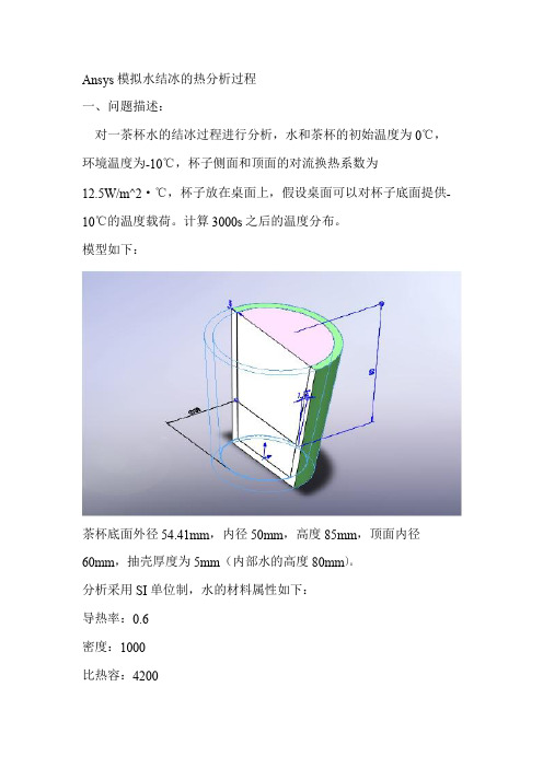
Ansys模拟水结冰的热分析过程一、问题描述:对一茶杯水的结冰过程进行分析,水和茶杯的初始温度为0℃,环境温度为-10℃,杯子侧面和顶面的对流换热系数为12.5W/m^2·℃,杯子放在桌面上,假设桌面可以对杯子底面提供-10℃的温度载荷。
计算3000s之后的温度分布。
模型如下:茶杯底面外径54.41mm,内径50mm,高度85mm,顶面内径60mm,抽壳厚度为5mm(内部水的高度80mm)。
分析采用SI单位制,水的材料属性如下:导热率:0.6密度:1000比热容:4200/prep7!进入前处理模块et,1,70!定义70单元mp,kxx,1,0.6!设置材料属性mp,c,1,4200mp,dens,1,1000mptemp,1,-10,-1,0,10mpdata,enth,1,1,0,37.8e6,79.8e6,121.8e6!焓值定义mp,kxx,2,70mp,dens,2,7833mp,c,2,448这里定义1号材料为水,2号材料为茶杯3、定义参数r1=50e-3r2=60e-3r3=54.41e-3r4=65e-3h1=80e-3h2=85e-34、建模wprot,,-90!旋转工作平面/pnum,volu,1!打开体积显示/view,1,1,1,1!Iso视角cone,r1,r2,0,h2,0,90!建立水的1/4圆台模型cone,r3,r4,0,h2,0,90!建立茶杯轮廓模型wpoff,,,h2-h1!移动工作平面vsbw,all!用工作平面切割体,方便扫掠划分网格vovlap,all!对体进行叠分操作vglue,all!对体进行粘接操作numcmp,all!压缩所有编号wpcsys,-1,0!工作平面回归原点/replot!重新显示5、对体赋予材料属性vsel,,,,1,3!体积1到3vatt,2,,1!赋予2号材料属性vsel,,,,4!体积4vatt,1,,1!赋予1号材料属性Allsel!选择所有/pnum,mat,1!打开材料编号显示Vplot!模型显示模型显示如上,紫色部分为茶杯,材料属性2 6、分网esize,2.5e-3!单元尺寸2.5e-3vsweep,all!扫掠划分网格划分如上,可见网格密度还是可以接受的。
ANSYS热应力分析实例

6
设置材料属性
1.给定材料的导热系数40W/(m·℃) 。
Main Menu> Preprocessor> Material Props> Material Models
7
建立实体模型(国际单位制)
1. 创建矩形A1:x1,y1(0,0)、x2,y2(0.01,0.07) MainMenu>Preprocessor>Modeling>Create>Areas>Rectangle>By Dimensions 2. 创建矩形A2:x1,y1(0,0.05)、x2,y2(0.08,0.07) 3.显示面的编号 Utility Menu>PlotCtrls>Numbering 4. 对面A1和A2进行overlap操作 Main Menu>Preprocessor>Modeling>Operate>Booleans> Overlap>Areas
12
13
求解
Main Menu>Solution>Solve>Current LS
14
查看温度场分布
Main Menu>General Postproc>Plot Results>Contour Plot>Nodal Solu
15
16
保存
稳态温度场计算完毕,下面修改分析文件名称,进行热应力计算。
注:S标志表示对称约束。
28
求解
Main Menu>Solution>Solve>Current LS
29
查看计算结果
Main Menu>General Postproc>Plot Results>Contour Plot>Nodal Solu
ansys热分析实例教程
Temperature distribution in a CylinderWe wish to compute the temperature distribution in a long steel cylinder with inner radius 5 inches and outer radius 10 inches. The interior of the cylinder is kept at 75 deg F, and heatis lost on the exterior by convection to a fluid whose temperature is 40 deg F. The convection coefficient is 0.56 BTU/hr-sq.in-F and the thermal conductivity for steel is 0.69 BTU/hr-in-F.1. Start ANSYS and assign a job name to the project. Run Interactive -> set working directory and jobname.2. Preferences -> Thermal will show -> OK3. Recognize symmetry of the problem, and a quadrant of a section through the cylinder is created using ANSYS area creation tools. Preprocessor -> Modeling -> Create -> Areas -> Circle -> Partial annulusThe following geometry is created.4. Preprocessor -> Element Type -> Add/Edit/Delete -> Add -> Thermal Solid -> Solid 8 node 77 -> OK -> Close5. Preprocessor -> Material Props -> Isotropic -> Material Number 1 -> OKEX = 3.E7 (psi)DENS = 7.36E-4 (lb sec^2/in^4)ALPHAX = 6.5E-6PRXY = 0.3KXX = 0.69 (BTU/hr-in-F)6. Mesh the area and refine using methods discussed in previous examples.7. Preprocessor -> Loads -> Apply -> Temperatures -> NodesSelect the nodes on the interior and set the temperature to 75.8. Preprocessor -> Loads -> Apply -> Convection -> LinesSelect the lines defining the outer surface and set the convection coefficient to 0.56 and the fluid temp to 40.9. Preprocessor -> Loads -> Apply -> Heat Flux -> LinesTo account for symmetry, select the vertical and horizontal lines of symmetry and set the heat flux to zero.10. Solution -> Solve current LS11. General Postprocessor -> Plot Results -> Nodal Solution -> TemperaturesThe temperature on the interior is 75 F and on the outside wall it is found to be 45. These results can be checked using results from heat transfer theory.BackThermal Stress of a Cylinder using Axisymmetric ElementsA steel cylinder with inner radius 5 inches and outer radius 10 inches is 40 inches long and has spherical end caps. The interior of the cylinder is kept at 75 deg F, and heat is lost on the exterior by convection to a fluid whose temperature is 40 deg F. The convection coefficient is 0.56 BTU/hr-sq.in-F. Calculate the stresses in the cylinder caused by the temperature distribution.The problem is solved in two steps. First, the geometry is created, the preference set to'thermal', and the heat transfer problem is modeled and solved. The results of the heat transfer analysis are saved in a file 'jobname.RTH' (Results THermal analysis) when you issue a save jobname.db command.Next the heat transfer boundary conditions and loads are removed from the mesh, the preference is changed to 'structural', the element type is changed from 'thermal' to 'structural', and the temperatures saved in 'jobname.RTH' are recalled and applied as loads.1. Start ANSYS and assign a job name to the project. Run Interactive -> set working directory and jobname.2. Preferences -> Thermal will show -> OK3. A quadrant of a section through the cylinder is created using ANSYS area creation tools.4. Preprocessor -> Element Type -> Add/Edit/Delete -> Add -> Solid 8 node 77 -> OK ->Options -> K3 Axisymmetric -> OK5. Preprocessor -> Material Props -> Isotropic -> Material Number 1 -> OKEX = 3.E7 (psi)DENS = 7.36E-4 (lb sec^2/in^4)ALPHAX = 6.5E-6PRXY = 0.3KXX = 0.69 (BTU/hr-in-F)6. Mesh the area using methods discussed in previous examples.7. Preprocessor -> Loads -> Apply -> Temperatures -> NodesSelect the nodes on the interior and set the temperature to 75.8. Preprocessor -> Loads -> Apply -> Convection -> LinesSelect the lines defining the outer surface and set the coefficient to 0.56 and the fluid temp to 40.9. Preprocessor -> Loads -> Apply -> Heat Flux -> LinesSelect the vertical and horizontal lines of symmetry and set the heat flux to zero.10. Solution -> Solve current LS11. General Postprocessor -> Plot Results -> Nodal Solution -> TemperatureThe temperature on the interior is 75 F and on the outside wall it is found to be 43.12. File -> Save Jobname.db13. Preprocessor -> Loads -> Delete -> Delete All -> Delete All Opts.14. Preferences -> Structural will show, Thermal will NOT show.15. Preprocessor -> Element Type -> Switch Element Type -> OK (This changes the element to structural)16. Preprocessor -> Loads -> Apply -> Displacements -> Nodes(Fix nodes on vertical and horizontal lines of symmetry from crossing the lines of symmetry.)17. Preprocessor -> Loads -> Apply -> Temperature -> From Thermal AnalysisSelect Jobname.RTH (If it isn't present, look for the default 'file.RTH' in the root directory)18. Solution -> Solve Current LS19. General Postprocessor -> Plot Results -> Element Solution - von Mises StressThe von Mises stress is seen to be a maximum in the end cap on the interior of the cylinder and would govern a yield-based design decision.Back。
ANSYS流体与热分析第10章热分析典型工程实例
第10 章热分析典型工程实例本章要点拉伸特征旋转特征扫掠特征混合特征孔特征壳特征本章案例某型号手机电池的散热分析冷库复合隔热板热量流动分析电子元器件散热装置温度分析10.1 工程实例1——某型号手机电池的散热分析该算例为某型手机电池的散热分析,如图10-1为某型号手机背面的照片,图中可见手机的电池的位置。
在手机工作时,电池可向外传递热量。
使用手机的读者应该都体会过手机电池发热的现象,特别是在长时间接打电话时,这种现象尤为明显。
本实例对某型号手机进行分析,电池的标准电压为3.7V,电池容量为750mAh。
试求手机开机状态下外壳的温度分布。
手机的各部分材料性能参数如表10.1所示。
图10-1 手机背面照片在计算分析过程中我们将手机看做三个组成部分:塑料外壳、手机内部材料和手机电池。
忽略手机内部线路和芯片,可以将手机电池看做唯一热源。
简化后的手机模型如图10-2所示,图中单位均为cm。
本实例拟采用Solid Tet 10node 87单元进行分析。
由于电池功率和环境温度均可视为恒定不变,因此分析类型为稳态。
图10-2 简化后的手机模型由电池的电压和电流可以算得电池的功率:==⨯=P UI 3.70.75 2.775W电池的体积为:3=⨯⨯=V0.040.010.050.00002m电池的发热量:3==Q P/V138750W/m——附带光盘“Ch10\实例10-1_start”——附带光盘“Ch10\实例10-1_end”——附带光盘“A VI\Ch10\10-1.avi”1、定义分析文件名1、选择Utility Menu>File>Change Jobname,在弹出的单元增添对话框中输入Example10-1,然后点击OK按钮。
2、选择Main Menu>Preferences,弹出Preferences for GUI Filtering对话框,点选Thermal复选框,单击OK按钮关闭该对话框。
ansys热分析实例教程
Temperature distribution in a CylinderWe wish to compute the temperature distribution in a long steel cylinder with inner radius 5 inches and outer radius 10 inches. The interior of the cylinder is kept at 75 deg F, and heatis lost on the exterior by convection to a fluid whose temperature is 40 deg F. The convection coefficient is 0.56 BTU/hr-sq.in-F and the thermal conductivity for steel is 0.69 BTU/hr-in-F.1. Start ANSYS and assign a job name to the project. Run Interactive -> set working directory and jobname.2. Preferences -> Thermal will show -> OK3. Recognize symmetry of the problem, and a quadrant of a section through the cylinder is created using ANSYS area creation tools. Preprocessor -> Modeling -> Create -> Areas -> Circle -> Partial annulusThe following geometry is created.4. Preprocessor -> Element Type -> Add/Edit/Delete -> Add -> Thermal Solid -> Solid 8 node 77 -> OK -> Close5. Preprocessor -> Material Props -> Isotropic -> Material Number 1 -> OKEX = 3.E7 (psi)DENS = 7.36E-4 (lb sec^2/in^4)ALPHAX = 6.5E-6PRXY = 0.3KXX = 0.69 (BTU/hr-in-F)6. Mesh the area and refine using methods discussed in previous examples.7. Preprocessor -> Loads -> Apply -> Temperatures -> NodesSelect the nodes on the interior and set the temperature to 75.8. Preprocessor -> Loads -> Apply -> Convection -> LinesSelect the lines defining the outer surface and set the convection coefficient to 0.56 and the fluid temp to 40.9. Preprocessor -> Loads -> Apply -> Heat Flux -> LinesTo account for symmetry, select the vertical and horizontal lines of symmetry and set the heat flux to zero.10. Solution -> Solve current LS11. General Postprocessor -> Plot Results -> Nodal Solution -> TemperaturesThe temperature on the interior is 75 F and on the outside wall it is found to be 45. These results can be checked using results from heat transfer theory.BackThermal Stress of a Cylinder using Axisymmetric ElementsA steel cylinder with inner radius 5 inches and outer radius 10 inches is 40 inches long and has spherical end caps. The interior of the cylinder is kept at 75 deg F, and heat is lost on the exterior by convection to a fluid whose temperature is 40 deg F. The convection coefficient is 0.56 BTU/hr-sq.in-F. Calculate the stresses in the cylinder caused by the temperature distribution.The problem is solved in two steps. First, the geometry is created, the preference set to'thermal', and the heat transfer problem is modeled and solved. The results of the heat transfer analysis are saved in a file 'jobname.RTH' (Results THermal analysis) when you issue a save jobname.db command.Next the heat transfer boundary conditions and loads are removed from the mesh, the preference is changed to 'structural', the element type is changed from 'thermal' to 'structural', and the temperatures saved in 'jobname.RTH' are recalled and applied as loads.1. Start ANSYS and assign a job name to the project. Run Interactive -> set working directory and jobname.2. Preferences -> Thermal will show -> OK3. A quadrant of a section through the cylinder is created using ANSYS area creation tools.4. Preprocessor -> Element Type -> Add/Edit/Delete -> Add -> Solid 8 node 77 -> OK ->Options -> K3 Axisymmetric -> OK5. Preprocessor -> Material Props -> Isotropic -> Material Number 1 -> OKEX = 3.E7 (psi)DENS = 7.36E-4 (lb sec^2/in^4)ALPHAX = 6.5E-6PRXY = 0.3KXX = 0.69 (BTU/hr-in-F)6. Mesh the area using methods discussed in previous examples.7. Preprocessor -> Loads -> Apply -> Temperatures -> NodesSelect the nodes on the interior and set the temperature to 75.8. Preprocessor -> Loads -> Apply -> Convection -> LinesSelect the lines defining the outer surface and set the coefficient to 0.56 and the fluid temp to 40.9. Preprocessor -> Loads -> Apply -> Heat Flux -> LinesSelect the vertical and horizontal lines of symmetry and set the heat flux to zero.10. Solution -> Solve current LS11. General Postprocessor -> Plot Results -> Nodal Solution -> TemperatureThe temperature on the interior is 75 F and on the outside wall it is found to be 43.12. File -> Save Jobname.db13. Preprocessor -> Loads -> Delete -> Delete All -> Delete All Opts.14. Preferences -> Structural will show, Thermal will NOT show.15. Preprocessor -> Element Type -> Switch Element Type -> OK (This changes the element to structural)16. Preprocessor -> Loads -> Apply -> Displacements -> Nodes(Fix nodes on vertical and horizontal lines of symmetry from crossing the lines of symmetry.)17. Preprocessor -> Loads -> Apply -> Temperature -> From Thermal AnalysisSelect Jobname.RTH (If it isn't present, look for the default 'file.RTH' in the root directory)18. Solution -> Solve Current LS19. General Postprocessor -> Plot Results -> Element Solution - von Mises StressThe von Mises stress is seen to be a maximum in the end cap on the interior of the cylinder and would govern a yield-based design decision.Back。
ANSYS_热分析报告(两个实例)有限元热分析报告上机指导书
第四讲 热分析上机指导书CAD/CAM 实验室,USTC实验要求:1、通过对冷却栅管的热分析练习,熟悉用ANSYS 进展稳态热分析的根本过程,熟悉用直接耦合法、间接耦合法进展热应力分析的根本过程。
2、通过对铜块和铁块的水冷分析,熟悉用ANSYS 进展瞬态热分析的根本过程。
容1:冷却栅管问题问题描述:本实例确定一个冷却栅管〔图a 〕的温度场分布与位移和应力分布。
一个轴对称的冷却栅结构管为热流体,管外流体为空气。
冷却栅材料为不锈钢,特性如下:W/m ℃×109 MPa×10-5/℃边界条件:〔1〕管:压力:6.89 MPa流体温度:250 ℃对流系数249.23 W/m 2℃〔2〕管外:空气温度39℃对流系数:62.3 W/m 2℃假定冷却栅管无限长,根据冷却栅结构的对称性特点可以构造出的有限元模型如图b 。
其上下边界承受边界约束,管部承受均布压力。
练习1-1:冷却栅管的稳态热分析步骤:1. 定义工作文件名与工作标题1) 定义工作文件名:GUI: Utility Menu> File> Change Jobname ,在弹出的【ChangeJobname 】对话框中输入文件名Pipe_Thermal ,单击OK 按钮。
2) 定义工作标题:GUI: Utility Menu> File> Change Title ,在弹出的【Change Title 】对话框中2D Axisymmetrical Pipe Thermal Analysis ,单击OK 按钮。
3) 关闭坐标符号的显示:GUI: Utility Menu> PlotCtrls> Window Control> WindowOptions ,在弹出的【Window Options 】对话框的Location of triad 下拉列表框中选择No Shown 选项,单击OK 按钮。
- 1、下载文档前请自行甄别文档内容的完整性,平台不提供额外的编辑、内容补充、找答案等附加服务。
- 2、"仅部分预览"的文档,不可在线预览部分如存在完整性等问题,可反馈申请退款(可完整预览的文档不适用该条件!)。
- 3、如文档侵犯您的权益,请联系客服反馈,我们会尽快为您处理(人工客服工作时间:9:00-18:30)。
问题描述:一个30公斤重、温度为70℃的铜块,以及一个20公斤重、温度为80℃的铁块,突然放入温度为20℃、盛满了300升水的、完全绝热的水箱中,如图所示。
过了一个小时,求铜块与铁块的最高温度(假设忽略水的流动)。
材料热物理性能如下:热性能单位制铜铁水导热系数W/m℃ 383 37密度Kg/m 8889 7833 996比热J/kg℃ 390 448 4185菜单操作过程:一、设置分析标题1、选择“Utility Menu>File>Change Jobname”,输入文件名Transient1。
2、选择“Utility Menu>File>Change Title”输入Thermal Transient Exercise 1。
二、定义单元类型1、选择“Main Menu>Preprocessor”,进入前处理。
2、选择“Main Menu>Preprocesor>Element Type>Add/Edit/Delete”。
选择热平面单元plane77。
三、定义材料属性1、选择“Main Menu>Preprocessor>Material Props>Material Models”,在弹出的材料定义窗口中顺序双击Thermal选项。
2、点击Conductivity,Isotropic,在KXX框中输入383;点击Density,在DENS框中输入8898;点击Specific Heat,在C框中输入390。
3、在材料定义窗口中选择Material>New Model,定义第二种材料。
4、点击Conductivity,Isotropic,在KXX框中输入70;点击Density,在DENS框中输入7833;点击Specific Heat,在C框中输入448。
5、在材料定义窗口中选择Material>New Model,定义第三种材料。
6、点击Conductivity,Isotropic,在KXX框中输入.61;点击Density,在DENS框中输入996;点击Specific Heat,在C框中输入4185。
四、创建几何模型1、选择“Main Menu>Preprocessor>-Modeling->Create>-Areas->Retangle>By Dimensions”,输入X1=0, Y1=0, X2=, Y2=, 点击Apply;输入X1=, Y1=, X2= ,Y2=, 点击Apply;输入X1= Y1=, X2= Y2=+, 选择OK。
2、选择“Main Menu>Preprocessor>-Modeling->Operate>Booleans>Overlap”,选择Pick All。
3、选择“Utility Menu>Plotctrls>Numbering>Areas, on”。
4、选择“Utility Menu>Plot>Areas”。
五、划分网格1、选择“Main Menu>Preprocessor>-Attributes->Define->All Areas”,选择材料1。
2、选择“Main Menu>Preprocessor>Meshing->Size Cntrls->-Manualsize->-Global->Size”,输入单元大小。
3、选择“Main Menu>Preprocessor>Meshing->Mesh->-Areas->Mapped>3 or 4 sided”,选择铜块。
4、选择“Main Menu>Preprocessor>-Attributes->Define->All Areas”,选择材料2。
5、选择“Main Menu>Preprocessor>Meshing->Mesh->-Areas->Mapped>3 or 4 sided”,选择铁块。
6、选择“Main Menu>Preprocessor>-Attributes->Define->All Areas”,选择材料3。
7、选择“Main Menu>Preprocessor>Meshing->Size Cntrls->-Manualsize->-Global->Size”,输入单元大小。
8、选择“Main Menu>Preprocessor>Meshing->Mesh->-Areas->Free”,选择水箱。
9、选择“Utility Menu>Plot>Area”。
六、进行稳态分析设置初始条件1、选择“Main Menu>Solution>-Analysis Type->New Analysis”,选择Transient,定义为瞬态分析。
2、选择“Main Menu>Solution>-Load Step Opts>Time/Frenquenc>Time Integration”,将TIMINT设定为 off,首先进行稳态分析。
3、选择“Main Menu>Solution>-Load Step Opts>Time/Frenquenc>Time-Time Step”,设定TIME为、DELTIM也为4、选择“Utility Menu: Select>Entities”,在对话框中自上而下依次选择:Elements,By Attributes,Material num,在“Min, Max”框中输入3,选择From Full,点击APPLY;选择选择Nodes,Attached to, Element,点击OK。
5、选择“Main Menu>Solution>-Loads->Apply>-Thermal->Temperature>On Nodes”,选择Pick All, 输入20。
6、选择“Utility Menu: Select>Entities”,在对话框中自上而下依次选择:Elements,By Attributes,Material num,在“Min, Max”框中输入2,选择From Full,点击APPLY;选择选择Nodes,Attached to, Element,点击OK。
7、选择“Main Menu>Solution>-Loads->Apply>-Thermal->Temperature>On Nodes”,选择Pick All, 输入80。
8、选择“Utility Menu>Select>Entities”,在对话框中自上而下依次选择:Elements,By Attributes,Material num,在“Min, Max”框中输入1,选择From Full,点击APPLY;选择选择Nodes,Attached to, Element,点击OK。
9、选择“Main Menu>Solution>-Loads->Apply>-Thermal->Temperature>On Nodes”,选择Pick All, 输入70。
10、选择“Utility Menu>Select Everything”。
11、Main Menu>Solution>-Solve->Current LS”。
七、进行瞬态分析1、选择“Main Menu>Solution>-Load Step Opts>Time/Frenquenc>Time-Time Step”,设定TIME=3600,DELTIM=26, 最小、最大时间步长分别为2, 200, 将Autots设置为ON。
2、选择“Main Menu>Solution>-Load Step Opts>Time/Frenquenc>Time Integration”,将TIMINT设置为ON。
3、选择“Main Menu>Solution>-Loads->Delete>-Thermal->Temperature>On Nodes”,选择Pick All,删除稳态分析定义的节点温度。
4、选择“Main Menu>Solution>-Load Step Opts>Output Ctrls->DB/Results”,选择Every Substeps。
5、选择“Main Menu>Solution>-Solve->Current LS”。
八、后处理1、选择“Main Menu>TimeHist PostPro”,进入POST26。
2、选择“Main Menu>TimeHist PostPro>Define Variables”,点击Add,选择Solution summary,点击OK,在User specified label框中输入dtime,选择Solution Items和StepTime,点击OK定义子步时间为2号变量。
3、选择“Main Menu>TimeHist PostPro>Define Variables”,点击Add,选择Nodal result,点击OK,在User specified label框中输入T_Copper,在Node number框中输入node,,0),点击OK定义3号变量。
同理可以定义其他节点解。
4、选择“Main Menu>TimeHist PostPro>Graph Virables”,输入变量代号,显示各变量随时间变化的曲线。
5、选择“Main Menu>General Postproc”,进入POST1。
6、选择“Main Menu>General Postproc>-Read Results->Last set”。
7、选择“Main Menu>General Postproc>Plot result>Nodal Solution”,选择temperature。
等效的命令流方法/filename,transient1/title, Thermal Transient Exercise 1!进入前处理/prep7et,1,plane77! 定义单元类型mp,kxx,1,383! 定义材料热性能参数mp,dens,1,8889!1~铜,2~铁,3~水mp,c,1,390mp,kxx,2,70mp,dens,2,7837mp,c,2,448mp,kxx,3,mp,dens,3,996mp,c,3,4185!创建几何实体rectnag,0,,0,rectang,,,,rectang,布尔操作/pnum,area,1aplot!划分网格aatt,1,1,1eshape,2esize,amesh,2aatt,2,1,1amesh,3aatt,3,1,1eshape,3esize,amesh,4/pnum,mat,1eplotfinish/soluantype,transtimint,off!先作稳态分析,确定初始条件time,!设定只有一个子步的时间很小的载荷步deltim,esel,s,mat,,3nsle,sd,all,temp,20esel,s,mat,,2nsle,sd,all,temp,80esel,s,mat,,1nsle,sd,all,temp,70allselsolve!得到初始温度分布!进行瞬态分析time,3600timint,on!打开时间积分deltim,26,2,200!设置时间步长,最大及最小时间步长autots,on!打开自动时间步长ddelet,all,temp!删除稳态分析中定义的节点温度outres,all,1!将每个子步的值写入数据库文件solvefinishsave!进入POST26后处理/post26solu,2,dtime,,dtime!2~每一子步采用的时间步长nsol,3,node,,0),temp,,T_Copper!3~铜块的中心点nsol,4,node,,0),temp,,T_Iron!4~铁块的中心点nsol,5,node(30,0,0),temp,,T_H2O_Bot!5~水箱的底部nsol,6,node(30,50,0),temp,,T_H2O_Top!6~水箱的顶部nsol,7,node(0,25,0),temp,,T_H2O_Left!7~水箱的左部nsol,8,node(60,25,0),temp,,T_H2O_Right!8~水箱的右部Plvar,2plvar,3,4,5,6,7,8finish!进入POST1后处理/post1!设置为最后一个载荷子步set,lastesel,s,mat,,1nsle,sesel,s,mat,,2 nsle,s plnsol,temp finish。