Automatic optimisation of parallel linear algebra routines in systems with variable load
Edwards nEXT涡流式瓶颈泵产品说明书

nEXT TURBOMOLECULAR PUMPSINNOVATION AND RELIABILITYEdwards nEXT is the ultimate experience in turbomolecular pumps. nEXT turbomolecular pumps are built on decades of experience and are drawing from our tried and trusted EXT and STP ranges. nEXT pumps offer superior performance, reliability and end user serviceability, setting the benchmark for scientific turbomolecular pumps.nEXT has been designed to combine all the latest technological advances in turbomolecular pumps with some new thinking in design for manufacture, delivering a truly class leading product.The nEXT platform brings a high level of modularity to offer maximum flexibility for customer application and requirements. Each pump is available in different internal configurations to offer differing functionality and performance.Our nEXT pumps come in different variants "D" Duplex comes with both turbomolecular and drag stages for improved tolerance to higher backing line pressures. The “D” variants offer superior pumping speed and compression across all gas species. Triplex “T” variants feature turbomolecular, drag and Edwards unique regenerative pumping stages for the ultimate in compression ratio and boost technology for unique vacuum system rationalisation.The "H" variant has been physically tuned to offer an improvement where an application has focus on light gas compression.Exceptional pumping speeds and compression ratios Huge install base of turbo pumps Bespoke design service available Integrated intelligent controls Fully end user serviceable Enhanced customer choiceADVANCED TECHNOLOGY Superior performance Proven reliability for peace of mind Flexible solutionsEase of useExtended lifetime and low cost of ownershipLarge variety of standard variantsApplicationsResearch & DevelopmentChamber evacuation, coating systems, turbomolecular pump systemsHigh Energy PhysicsBeam lines, accelerators, mobile pump carts, turbomolecular pump backing, laser evacuation, medical systemsMass SpectrometryGCMS, LCMS, ICPMS, MALDI, inorganic MS, RGA, surface science, leak detectorsElectron MicroscopyTEM, SEM, EPMA, SPM sample prep benchesIndustrialGlove boxes, coating systems, XRD/XRF systems, leak testing, energy, furnaces, medical technologiesYou can be assured Edwards has the application expertise and vacuum solution to meet your needs.Inlet flange sizesnEXT55D x*x x x*nEXT85D nEXT85H x x x xnEXT240D nEXT240T x xnEXT300D nEXT300T x xnEXT400D nEXT400T x xnEXT730D x x x xnEXT930D x xnEXT1230H x x x *Available by special orderPERFORMANCE YOU CAN RELY ONFor higher compression ratios and greater backing pressure toleranceEnables wider operating envelope (nEXT55-nEXT85)Enables boost port options and higher compression (nEXT240, 300, 400)Minimises noise and vibration transmitted to vacuum (nEXT240, 300, 400)For a speedy interim service and bearing cartridge for a quick low cost scheduled overhaul (nEXT55-400)For safe operation of pump with specialised gasesFor a hydrocarbon free vacuum, reduced vibration and minimum wear Derived rotor design to give better speed and compression performanceWith automatic valve accessories for rapid venting and quick cycle timesFor flexible system tuningOr more sophisticated serial control in both RS232 and RS485 protocolsFrom 24V to 48V d.c. for versatility in system integration (nEXT730-1230 48V)For high efficiency and compactness with reduced stray magnetic fields1 - Multiple drag stages2 - Direct temperature measurements within the pump3 - Third regenerative stage4 - Patented bearing suspension system5 - User replaceable oil cartridge6 - Purge port7 - Permanent magnet upper bearing 8 - Advanced simulation tool9 - Manual vent port10 - Manual as well as serial setting of standby speed11 - Simple parallel operation12 - Automatic wide operating voltage range13 - Sensorless drivenEXT55 AND nEXT85The most compact pumps of the nEXT range with a significantly reduced height and improved performance in a smaller package.These pumps offer pumping speeds of 55 l/s and 85 l/s for nitrogen, they provide a high pumping density, greater than other pumps in its class, with almost double the pumping speed of similar sized turbo pumps.As with all the pumps in the nEXT range field maintenance is only required every 4 years of operation, and this including replacement of the bearing can be performed by the end user.nEXT55 and nEXT85 bring with them the benefits in flexibility with comprehensive communication and control options available, as well as a full set of accessories, the ideal choice in deployable instruments or portable applications where a compact footprint or lower weight are key factors.The rotor has been designed to optimise pump performance and achieve both higher speeds and higher compression while maintaining high levels of reliability and low risk to adoptors.nEXT240, nEXT300 & nEXT400The innovative pumps, designed to provide high vacuum performance in a compact size.Giving OEMs and end users a greater choice and theflexibility to tailor the most appropriate vacuum solution to meet their individual needs.- the D-Type combines turbo and drag stages;- the T-Type adds Edwards unique fluid dynamic stages and the option of additional booster ports for increased system rationalisation.See Boost technology custom interface splitflow variants are also available in three sizes for further vacuum system optimisation.The pumps feature a field replaceable oil cartridge and bearing assembly and the user is notified as to when service intervention is required.This enables easy maintenance as users can carry out servicing in-house, which reduces the cost of ownership.The efficient pumps have low power consumption and also feature a standby mode, which allow users to make further energy savings.nEXT240-300-400 pumps have extra low vibration and low magnetic field signature variants for sensitive electron microscope applications.The compact design means the pumps fit together neatly in high product density applications.They are easy to configure and have an intelligent control interface accepting a 24 to 48Vdc input power supply voltage range and can be controlled using a simple parallel control or serial communications in both RS232 or RS485 formats.A wide variety of sizesEach is available in two variantsField replaceable oil cartridge and bearing assembly Low power consumption and standby modeCompact designThe examples below shows how boost can be used to either reduce the size of the primarypump or increase the gas flow into the instrument on a differentially pumped system.It also illustrates how the number of turbo pumps required can be reduced from two discrete pumps to a single splitflow pump with two inlets to achieve the same vacuum performance.Customers in general laboratory and R&Dapplications will also benefit from the improved compression achieved with the "T" variant.To take maximum advantage of boost technology,please contact Edwards.Regenerative StageBOOST TECHNOLOGYA much simplified vacuum solution with greatly improved pumping speeds and system powerreductionOriginal SystemBoost Option 1Boost Option 2Screenshot taken from TransCalc HSMnEXT730, nEXT930 & nEXT1230Larger pumps offering nitrogen pumping speeds of 730, 925 and 1250 l/s respectively.As well as addressing the general R&D market, where high pumping speeds are often required, these pumps are also designed to meet the requirements of the coating market and other diffuse market sectors such as: - Heat treatment- Furnace applications- E-beam welding- Etch- Ion implant- Degassing- Cylinder evacuationFor our OEM customers, derivative versions of these products including split flow variants can be developed to match specific applications.These compact pumps are able to operate in any orientation, and are supported by a full range of accessories for cooling, venting, powering and control.When required, a bearing replacement can be undertaken by the customer themselves or they can take advantage of our other service support options.Designed to meet a wide range of requirementsWe match the specific applications of OEM Operate in any orientationThe pumps feature bearings with a typical life time of at least 4 years with no maintenance.At Edwards, it all starts with a vacuum expert gathering your application details!We want to understand what pressures you wish to achieve, what gas flows you have, how much space is available etc.Our expert then uses a number of in-house and publicly available modelling tools at his disposal to optimise your vacuum system. Developed by our Analytical Services group, these tools are used to model complete vacuum systems fromatmosphere down to ultra-high vacuum (UHV).This software has been developed to give rapid simulation of the behaviour of the proposedvacuum solution to ensure that it perfectly meets your requirements.Accurate computer modelling offers you the chance to streamline your development cycle,avoiding a costly iterative approach and delivering a quicker time to market. Please contact Edwards to take advantage of this service.A partnership approach to system designWhen an off the shelf pump will not meet your requirements for space or performance, our Bespoke Product Development (BPD) team will develop a customised vacuum solution to turn your requirement into reality.Automatically recognises and supports oneturbomolecular pump from the nEXT range, one backing pump (nXDS or diaphragm) plus three Edwards active gauges on top of that cooling and vent valve support is provided directly from the controller. Backing pump power is provided for a compact 24V diaphragm pump (on 200W versions only), or where greater pumping speeds are required, nXDS and large XDS pumps can be controlled directly via the backing pumpconnector on a TIC 200 mains backing pumps (up to RV12) may be controlled via an optional relay box.The relay box can also be used to control a mains heater band and backing line isolation valve. Time delays and normal speed signals may be used to control events such as turbo start and there is a comprehensive selection of protection and safety interlock features. The TIC turbo controller may be either rack or bench mounted and provides a useful hub for the flexible operation of a wide range of vacuum system configurations.TICTurbo and Instrument ControllerA small, compact, low cost pumping system controller, which is suitable for a wide range of vacuum applications. It is a 24V controller that is compatible with all Edwards nEXT turbomolecular pumps. In addition to a turbomolecular pump it can control a backing pump, a vent valve, an air cooler and an Edwards active gauge. The TAG is controlled by an easy to use interface. A large clear LED display shows the pump speed or vacuum pressure. The compact size of thecontroller is ideal for use on benchtops or suitable mobile platforms.TAGTurbo and Active GaugeAn oil lubrication cartridge change can beperformed where fitted, typically in less than 5minutes. A full bearing change can also beperformed by the end user in around 10 minutes on all nEXT pumps. Both with the minimum of specialist tooling. These simple interventions will,in many cases, mean that the pump never requires a full return to base service during its lifetime.nEXT turbomolecular pumps will advise the user when a service is due and what level of intervention is required.The user is alerted to a service request by a simple flashing LED sequence on the pumps and by serial comms notification.Flexibility is again key as these simple services can be performed either by the end user, on site by an Edwards field service technician, or the pump can be returned to an Edwards service hub.Using remote diagnostics, a user can interrogate the pump to determine how long it is to the next service so that a proactive approach to preventative maintenance can be planned.End user serviceabilityNew technologies employed in nEXT have enabled the pumps to be serviced by the enduser in the field.Should a fault occur as a result of a manufacturing defect, equipment is expressly repaired or replaced.Cover is available on many of our products allowing the original factory warranty to beextended from 12 months to 2 years and beyond.Prolonged peace of mindExtending the new equipment warranty gives you a simple opportunity to add peace of mind to your purchase of new equipmentEdwards has a number of major service facilities located throughout the world, each location is supported by an extensive team of engineers and technicians to provide local, rapid response and great value service.All our service operations are conducted at the highest international standards in accordance with ISO9001 (Quality), ISO14001 (Environmental), and OHSAS18001 (Workplace safety).Your global partnerWe understand the importance of local support.Inlet flange DN63 ISO-K or DN63 CF NW40DN63 ISO-K or DN63 CF DN100 ISO-KInlet pumping speed ls-1N255478486Ar55448084He41617880/78 (D/H) H22749/44 (D/H)60/54 (D/H)60/54 (D/H)Compression ratio (D)N2/Ar>1 x 1011He 6.9 x 1058 x 106 H2 2.9 x 10⁴ 2 x 10⁵Compression ratio (T/H)N2/Ar NA>1 x 10¹¹ He NA 2 x 10⁷ H2NA 5 x 10⁵Backing/interstage/boost ports NW16Vent/purge port1/8” BSPPCritical backing pressure (D/H)mbar18Critical backing pressure (T)mbar NABake out water cooled/forced air cooled max.°C120/115°Recommended backing pump*nXDS6iNormal rotational speed (rpm)90,000Start time to 90% speed (sec) D/H (T)90Mass (kg) D/H (T)ISO 2.47 2.9 3.0 3.2CF 3.5 4.4*A smaller backing pump may be used depending on application.nEXT55, nEXT85Inlet flange DN100 ISO-K or DN100 CF DN100 ISO-K or DN100 CF DN160 ISO-K or DN160 CFInlet pumping speed ls-1N2240300400 Ar230280380 He230340390 H2165280325Compression ratio (D)N2/Ar>1 x 1011>1 x 10¹¹>1 x 10¹¹ He 3 x 10⁵ 1 x 10⁶ 1 x 10⁸ H2 1 x 10⁴ 5 x 10⁴ 5 x 10⁵Compression ratio (T/H)N2/Ar>1 x 1011>1 x 10¹¹>1 x 10¹¹ He 1 x 10⁶ 3 x 10⁶>1 x 10⁸ H2 1.5 x 10⁴ 1 x 10⁵ 1 x 10⁶Backing/interstage/boost ports NW25NW25NW25Vent/purge port1/8” BSPP1/8” BSPP1/8” BSPPCritical backing pressure (D/H)mbar9.59.510Critical backing pressure (T)mbar202020Bake out water cooled/forced air cooled max.°C120/115°120/115°120/115°Recommended backing pump*RV12/nXDS10i RV12/nXDS10i RV12/nXDS10i Normal rotational speed (rpm)60,00060,00060,000Start time to 90% speed (sec) D/H (T)115 (150)145 (190)180 (210)Mass (kg) D/H (T)ISO 5.7 (6) 5.7 (6) 6.5 (6.8)CF8.8 (9.1)8.5 (8.8)9.5 (9.8)* A smaller backing pump may be used depending on application.Inlet flange DN 160 ISO-K DN 160 CF DN 200 ISO-K DN 200 CF DN 200 CF DN 200 ISO-F DN 200 ISO-KInlet pumping speed ls-1N27309251250 Ar6658651150 He8209051350 H27157351150Gas throughput mbar ls-1N2141412 nEXT730, nEXT930, nEXT1230Gas throughput mbar ls-1Ar 3.5 3.54 He2121>20 H2>>14>>14>20Compression ratio N2>1 x 10¹¹Ar>1 x 10¹¹He 1.2 x 10⁸ 1.2 x 10⁸ 4 x 10+8 H2 4 x 10⁶ 4 x 10⁶ 1 x 10+7Ultimate pressure with 2-stage oil sealed rotary vane pump ISO-K/CF mbar<3.5 x 10⁻⁹<6 x 10⁻¹⁰<3.5 x 10⁻⁹<6 x 10⁻¹⁰<5 x 10⁻¹⁰<5 x 10⁻⁹ Backing/interstage/boost ports NW40Normal rotational speed rpm49 20049 20042 000Start time to 90% speed (sec) D/H (T)min 2.5 2.53Cooling water consumption l/h60Critical backing pressure mbar15Mass (kg) D/H (T)kg14.619.615.421.732.624.923.7 Recommended backing pump*nXRi, XDS35i, E2M28*Bake out water cooled/forced air cooled max.°C n/a100n/a100100n/a n/a Vent/purge port G1/8”*Please contact your local representative to discuss the correct option for your application.PumpsnEXT55D NW40 NW16 80W B8E210A01 nEXT55D CF63 NW16 80W B8E210C01 nEXT55D ISO63 NW16 80W B8E210B01 nEXT55D ISO100 NW16 80W B8E210101 nEXT85D ISO63 NW16 80W B8G210B01 nEXT85D CF63 NW16 80W B8G210C01 nEXT85D ISO100 NW16 80W B8G210101 nEXT85D NW40 NW16 80W B8G210A01 nEXT85D ISO100 NW25 80W B8G240101 nEXT85iD ISO63 NW16/16 80W B8G211B01 nEXT85iD ISO63 NW16/25 80W B8G214B01 nEXT85H ISO63 NW16 80W B8G410B01 nEXT85H CF63 NW16 80W B8G410C01 nEXT85H NW40 NW16 80W B8G410A01 nEXT85iH CF63 NW16/16 80W B8G411C01 nEXT85H ISO100 NW16 80W B8G410101 nEXT240D ISO-K100 160W B81200100 nEXT240D CF100 160W B81200200 nEXT240T ISO-K100 160W B81300100 nEXT240T CF100 160W B81300200 nEXT300D ISO-K100 160W B82200100 nEXT300D CF100 160W B82200200 nEXT300T ISO-K100 160W B82300100 nEXT300T CF100 160W B82300200 nEXT400D ISO-K160 160W B83200300 nEXT400D CF160 160W B83200400 nEXT400T ISO-K160 160W B83300300nEXT400T CF160 160W B83300400nEXT730D ISO-K160 NW25B8J200300nEXT730D CF160 NW25B8J200400nEXT930D ISO-K200 NW25B8K200D00nEXT930D CF200 NW25B8K200F00nEXT1230H CF200 NW40B8N4A0F00nEXT1230H ISO-F200 NW40B8N4A0E00nEXT1230H ISO-K200 NW40B8N4A0D00nEXT1230H CF200 NW40 INV B8N4A0FU0nEXT1230H ISO-F200 NW40 INV B8N4A0EU0nEXT1230H ISO-K200 NW40 INVB8N4A0DU0Other insterstage port positions available upon requestController (-1)TAG controllerD3*******TAG power supplyD3*******TIC 200 turbo and instrument controller D3*******CoolingWCX85 water cooling kit (4 position)B8G200833ACX85 air cooler connector fitted B8G200820VentingN/O TAV5 vent valve connector fittedB8G200834N/C TAV5 vent valve connector fittedB8G200835BakeoutCF63 flange heater 110 VB8G200823CF63 flange heater 240 VB8G200824ServiceOil cartridge kitB8G200828Bearing and oil cartridge kit B8G200811Bearing replacement tool kitB8G200845MiscellaneousAccessory Y adaptorB8G200837Accessory cable 90 degree/extensionB8G200836Accessory connector bare wired B8G200839nEXT85/EXT75DX base mounting adaptorB8G200838(1) Denotes need second annotation nEXT730 and bigger pumps need their own power supply required accessory. Others optional depending on application.PumpsAccessories and spares nEXT55/85Controller(-1)TAG controller D3*******TAG power supply D3******* TIC100 turbo and instrument controller D3*******Cooling nEXT radial air cooler B58053175 nEXT axial air cooler B58053185 nEXT water cooler B80000815Bakeout CF100 flange heater 100-120 V B58052773 CF100 flange heater 200-240 V B58052774 CF160 flange heater 100-120 V B58052775 CF160 flange heater 200-240 V B58052776Venting TAV5 solenoid operated vent valve B58066010ServiceOil cartridge tool kit B80000812 Bearing tool kit B80000805 Oil cartridge B80000811 Bearing and oil cartridge B80000810(1) Denotes need second annotation nEXT730 and bigger pumps need their own power supply required accessory. Others optional depending on application.ControllersTAG controller D3*******TAG power supply D3******* TIC100 turbo and instrument controller D3*******CoolingAir cooling radial nEXT730/930B8J200800 Air cooling radial nEXT1230B8J200801 Water cooling nEXT730/930, 1/4 inch B8J200820Venting N/O TAV5 vent valve connector fitted B8G200834 N/C TAV5 vent valve connector fitted B8G200835 Vent port adaptor B58066011Inlet screens Center ring w. prot. screen DN200 ISO-K coarse B8J200807 Center ring w. prot. screen DN200 ISO-K fine B8J200808 Coarse inlet screen DN 200 CF B8J200809 Fine inlet screen DN 200 CF B8J200810Accessories and spares nEXT730/930/123031Inlet screens CF160 coarse inlet screen B80000823 CF160 fine inlet screen B80000824 ISO160 coarse inlet screen B80000825 ISO160 fine inlet screen B80000826ServiceBearing replacement kit B8J200827Bearing replacement tooling B8J200845Mains input cable Mains input cable 3m EU B8J200812 Mains input cable 3m US B8J200813 Mains input cable 3m UK B8J200814Power supply to pumpnEXT 3m open end cable B8J200816nEXT 5m open end cable B8J200817EPS 800B8J200819 nEXT 3m extension cable for EPS 800B8J200824nEXT 5m extension cable for the EPS 800B8J2008252.5m EU EPS 800, IP54 protected B8J2008292.5m US NEMA 6-15P 250V EPS 800, IP54 protected B8J2008302.5m UK EPS 800, IP54 protected B8J200831 EPS 800 mount kit to place the power supply directly on the pump B8J200832Miscellaneous Accessory cable 90 degree/extension B8G200836 Accessory Y adaptor B8G200837 Accessory connector bare wired B8G200839(1) Denotes need second annotation nEXT730 and bigger pumps need their own power supply required accessory. Others optional depending on application.Extension cables 1 m pump to controller cable D3******* 3 m pump to controller cable D3******* 5 m pump to controller cable D3*******Power cables(-1)2 m electrical supply cable UK plug D4******* 2 m electrical supply cable EU plug D4******* 2 m electrical supply cable US plug D4*******Miscellaneous Vent port adaptor B58066011 Accessories and sparesnEXT TURBOMOLECULAR PUMPS (3601 0091 01)Accessories and sparesPRX10 purge restrictor B58065001MiscellaneousTIC relay D3*******(1) Denotes need second annotation nEXT730 and bigger pumps need their own power supply required accessory. Others optional depending on application.33 3601 0091 01 - November 2021. All rights reserved.Edwards and the Edwards logo are trademarks ofEdwards Limited. Whilst we make every effort to ensurethat we accurately describe our products and services,we give no guarantee as to the accuracy orcompleteness of any information. Edwards Ltd,registered in England and Wales No. 6124750,registered office: Innovation Drive, Burgess Hill, WestSussex, RH15 9TW, UK.Part of the Atlas Copco Group。
optimazation of foundry process

Application of a Multi Objective Genetic Algorithm and a Neural Network to the optimisation of foundry processes.G.Meneghetti *, V. Pediroda**, C. Poloni ***Engin Soft Trading Srl, Italy** Dipartiento di Energetica, Università di Trieste, ItalyAbstractAim of the work was the analysis and the optimisation of a ductile iron casting using the Frontier software. Five geometrical and technological variables were chosen in order to maximise three design objectives. The calculations were performed using the software MAGMASOFT, devoted to the simulation of foundry processes based on fluid-dynamics, thermal and metallurgical theoretical approaches. Results are critically discussed by comparing the traditional and the optimised solution.1. IntroductionA very promising field for computer simulation techniques is certainly given by the foundry industry. The possibility of reliably estimating both the fluid-dynamics, thermal and microstructural evolution of castings (from the pouring of the molten alloy into the mould till the complete solidification) and the final properties are very interesting. In fact if the final microstructure and then the mechanical properties of a casting can be predicted by numerical simulation, the a-priori optimisation of the process parameters (whose number is usually high) can be carried out by exploring different technological solutions with significant improvements in the quality of the product, managing of human and economical resources and time-savings.This approach is extremely new in foundry and in this work an exploratory project aimed at the process optimisation of an industrial ductile iron casting will be presented.2. The simulation of foundry processes and foundamental equationsFrom a theoretical point of view, a foundry process can be considered as the sequence of various events [1-4]:-the filling of a cavity by means of a molten alloy, as described by fluid-dynamics laws (Navier-Stokes equation),-the solidification and cooling of the alloy, according to the heat transfer laws (Fourier equation),-the solid state transformations, related to the thermodynamics and the kinetics.A full understanding of the whole foundry process requires an investigation throughout all these three phenomena. However under some hypotheses (regular filling of the mould cavity, homogeneous temperature distribution at the end of filling, etc.) the analyses of the solidification and the solid state transformation only can lead to reliable estimation of the final microstructure and of the properties of the casting.The accuracy in simulating the solidification process depends mainly on:- the use of proper thermophysical properties of the materials involved in the process, taking into account their change with temperature,- the correct definition of the starting and boundary conditions, with particular regard to the heat transfer coefficients.From a numerical point of view, the investigation of the solidification process could be carried out by means of a pure heat flow calculation described by Fourier’s law of unsteady heat conduction :∂∂ρ∂∂λ∂∂t ()x [x C T T p j j=However a more correct evaluation requires to incorporate the additional heat transport by convective movement of mass due to temperature dependent shrinkage of the solidifying mush.Doing that temperature-dependent density functions are needed, so that the shrinkage can be calculated basing on the actual temperature loss. The total metal shrinkage within one time interval will lead to a corresponding metal volume flowing from the feeder into the casting passing through the feeder-neck. The actual temperature distribution in the feeder neck can be calculated on the basis of the following equation :∂∂ρ∂∂ρ∂∂λ∂∂t ()x (u )x [x ]C T C T T S p j p j j j+=+where the second term on the left hand side of the equation is the convective term while the first one on the right hand side is the conductive term. S denotes the additional internal heat source. The additional heat transport by convective movement of mass means that feeding may last much longer than being calculated by heat flow based uniquely on conduction.Anyway, when the feeder-neck freezes to a certain temperature, the feeding mechanism locks.Therefore the solidification of any other portion of the cast, now insulated, will take place independently from one another and the feed metal required during solidification will come from the remaining liquid. The final volume shrinkage will result in a certain porosity, which typically will be located at the hot spots.From the point of view of the real industrial interest, the above phenomena and the related equations can be approached only numerically: in fact complex 3D geometries have to be taken into account, as well as manufacturing parameters ensuring compliance with temperature-dependent thermophysical properties of the materials, production and process parameters. Finite elements,finite differences, control volumes or a combination of these are typical methods implemented in the software packages [2-3].The final result of the simulation is the knowledge of the actual feeding conditions, which is the basis for correctly design the size of feeders. It must be recalled that this knowledge-based approach is often by-passed by the use of empirical rules and in most cases the optimisation of the feeder size is not really performed (so that the feeders are simply oversized) or it is carried out by means of expensive in-field trial-and-correction procedures.The analyses were performed by using the MAGMASOFT ® software, specifically devoted to the simulation of foundry processes, based on fluid-dynamics, thermal and metallurgical theoretical approaches. In particular MAGMASOFT has a module, named MAGMAIron, devoted to the simulation of mould filling, casting solidification, solid state transformation, with the related mechanical properties (such as hardness, tensile strength and Young Modulus) of cast irons [8]3. Optimisation toolFormally, the optimisation problem addressed can be stated as follows.Minimise: F j (X ) , j=1,nWith respect to:X Subject to c X i mi (;,≥=01X (F ),......X (F ),X (F n 21Where X is the design variables vector, F i(X) are the objectives, and c i(X) are the constraints. FRONTIER’s optimisation methods are based on Genetic Algorithms (GA) and hill climbing methods. These allow the user to combine the efficient local convergence of traditional hill climbers, with the strengths of GA’s, which are their robustness to noise, discontinuities and multimodal characteristic, their ability to address multiple objectives cases directly, and their suitability for parallelisation.GA GENERAL STRUCTURE. A GA has the following stages:1.initialise a population of candidate designs and evaluate them, then2.create a new population by selecting some individuals which reproduce or mutate, and evaluatethis new populationStage 2 is repeated until terminationGA MECHANISMS. Design variables are encoded into chromosomes by means of integer number lists. Though there is an inherent accuracy limitation in using integer values, this is not significant since accuracy can easily be refined using classical optimisation techniques. The initial selection of candidates is important especially when evaluations are so expensive that not many can be afforded in the total optimisation. Initialisation can be done in FRONTIER either by reading a user-defined set, or by random choice, or by using a Sobol algorithm [9] to generate a uniformly distributed quasirandom sequence. The optimisation can also be restarted from a previous population.The critical operators governing GA performance are selection, crossover reproduction, and reproduction by mutation.Four selection operators are provided, all based on the concept of Pareto dominance. They are; (1) Local Geographic Selection; (2) Pareto Tournament Selection; (3) Pareto Tournament Directional Selection; and (4) Local Pareto Selection. The user can choose from these though (4) is recommended for use with either type of crossover, and (2) to generate the proportion of the population which is sent to the next generation unmodified.Most emphasis in FRONTIER is on use of directional crossover, which makes use of detected direction of improvement, and has some parallels with the Nelder & Mead Simplex algorithm. Classical two-point crossover algorithm are also provided.Mutation is carried out when chosen, by randomly selecting a design variable to mutate, then randomly assigning a value from the set of all possibilities.In all cases, GA probabilities can be selected by the user, in place of recommended defaults, if desired. All the algorithm are described in more detail in [10].OPERATIONAL USER CHOICE. Traditional GA’s generate a complete new population of designs from an existing set, at each generation. This can be done in FRONTIER using its MOGA algorithm. An alternative strategy is to use steady state reproduction via a MOGASTD algorithm. In this case, only a few individuals are replaced at each generation. This strategy is more likely to retain best individuals. The FRONTIER algorithm removes any duplicates generated. Population size are under the user’s control. FRONTIER case study work has usually used population from 16 to 64, due to the computational expense of the design evaluations.Classical hill climbers can be chosen by the user not only the refine GA solution. They can be adopted from the start of the optimisation, if the user can formulate his problem suitably, and if he is confident that the condition are appropriate.Returning to the problem of expansive design evaluation, many research have made use of response surface. These interpolate a set of computed design evaluation. The surface can then be used to provide objective functions which are much faster to evaluate. Interpolation of nonlinear functions in many variables, using polynomial or spline functions, becomes rapidly intractable however. FRONTIER provides a response surface option based on use of a neural net, with two nodal planes.Tests have shown this to be an extremely effective strategy when closely combined with the GA to provide a continuous update to the neural net.FITNESS AND CONSTRAINTS HANDLING. The objective values themselves are used as fitness values. Optionally, the user can supply weights to combine these into a single quantity. Constraints are normally used to compute a penalty decrementing the fitness. Alternatively, the combined constraint penalty can be nominated as an extra objective to be minimised.PARALLELISATION OF GA. The multithreading features of Java have been used to parallelise FRONTIER’s GA’s. The same code is usable in a parallel or sequential environment, thus enhancing portability. Multithreading is used to facilitate concurrent design evaluations, with analyses executed in parallel as far as possible, on the user’s available computational resources.DECISION SUPPORT. Even where there are a number of conflicting objectives to consider, we are likely to went to choose only one design. The Pareto boundary set of designs provides candidates for the final choice. In order to proceed further, the designer needs to focus on the comparative importance of the individual objectives. The role of decision support in FRONTIER is to help him to do this, by moving to a single composite objective which combines the original objectives in a way which accurately reflect his preferences.LOCAL UTILITY APPROACH. A wide range of methods has been tried for multiple criteria decision making . The main FRONTIER technique used is the Local Utility Approach (LUTA)[11]. This avoids asking the designer to directly weight the objectives relative to each other (though he can if he wishes), but rather asks him to consider some of the designs which have already been evaluated, and state which he prefers, without needing to give reasons. The algorithm then proceeds in two stages. First it decides if the preferences give are consistent in themselves, and guides the designer to change them if they are not. Then, it proposes a ‘common currency’ objectives measure, termed a utility, this being the sum of a set of piecewise linear utility functions, one for each individual objective. The preference information which the designer has provided can then be stated as a set of inequality relations between the utilities of designs. The algorithm uses the feasible region formed by these constraints to calculate the most typical composite utility function which is consistent with the designer’s preferences.This LUTA technique can be invoked after accumulating a comprehensive set of Pareto boundary designs as a result of a number of optimisation iterations. The advantage of the latter approach is that the focusing of attention on the part of the Pareto boundary which is of most interest can result in considerable computational saving, by avoiding computing information on the whole boundary. In practice so far in FRONTIER, we have generally used the LUTA technique after a set number of design evaluations, after which the utility function for a local hill climber to rapidly refine a solution.4. Object of the study and adopted optimisation procedureThe component investigated is a textile machine guide, for which both mechanical and integrity requirements are prescribed. Such requirements are satisfied, respectively, by reaching proper hardness values and by minimising the porosity content. Furthermore, from the industrial point of view, it is fundamental to maximise the process yield, lowering the feeder size.The chemical composition of the ductile iron is the following :C Si Mn P S Cu Sn Ni Cr Mg3.55 2.770.130.0380.00370.0480.0450.0170.0300.035The liquidus and solidus temperatures are 1155°C and 1120°C respectively. The thermo-physical properties of the material (thermal conductivity, density, specific heat, viscosity) are already implemented into the MAGMASOFT Materials Database.The GA optimisation process was performed starting from a configuration of the casting system which is already the result of the foundry practise optimisation.Only the solidification process was taken into account for the simulation, since it was considered to be more affected by the technological variables selected. Therefore the temperature of the cast at the beginning of the solidification process was set as a constant. Moreover the gating system was neglected in the simulation since its influence on the heat flow involved in the solidification process was thought to be negligible. As a consequence the numerical model considers only the cast, the feeder and the feeder-neck (see Fig. 1, referred to the starting casting system). The adopted mesh was chosen in such a way to balance the accuracy and the calculation time. As a consequence a number of metal cells ranging from 9000 to 12000 (resulting in a total number of cells approximately equal to 200000) was obtained in any analysed model.Five technological variables governing the solidification process have been taken into account and the respective ranges of possible variation were defined:1.temperature of the cast at the beginning of the solidification process , 1300 °C <T init.< 1380°C;2.heat transfer coefficients (HTC) between cast and sand mould , 400 W/m2K <HTC< 1200W/m2K;3.feeder height, 80 mm <H f< 180 mm4.feeder diameter, 30 mm<D f < 80 mm5.section area of the feeder-neck, 175 mm2 <A n< 490 mm2.These variables were considered to be representative of the foundry technology and significant in order to optimise the following design objectives :1.Hardness of the material in a particular portion of the cast2.casting weight (i.e. raw cast + feeder + feeder-neck)3.porosityAim of the analysis was to maximise the hardness and to minimise the total casting weight and the porosity. No constraints were defined for this analysis.Generally speaking, the optimisation procedure should be performed running one MAGMA simulation for each generated individual. That implies the possibility to assign all the input parameters and start the analysis via command files. Similarly the output files should be available in the form of ascii files from which the output parameters can be extracted. However at this stage a complete open interface between MAGMASOFT and Frontier is not still available. As a consequence another solution was adopted. First of all 64 analyses were performed in order to get sufficient information in all the variable domain. After that a interpolation algorithm was used to build a response surface model basing on a Neural Network, “trained” on the available results. It has been verified that the approximation reached is lower than 1% for all the available set of solutions with the exception of one point only where the approximation is slightly lower than 5%. After that the response surface model was used in the next optimisation procedure to calculate the design objectives. In such a way further time-expensive work needed to run one MAGMASOFT interactive session for each simulation was avoided.Concerning the Genetic Algorithm a mix between a classical and directional cross-over was used. The first population was created in a deterministic way.5. Results and discussionThe first optimisation task was done for 4 generations with 16 individuals for each generation. Since a complete simulation required about 20 minutes of CPU time on a workstation HP C200, the total CPU time resulted in about 21 hours and 20 minutes. Figs. 3, 4 and 5 report the obtained solutions. In particular from the tables it can be noted that the hardness values increase as we move from the first to the fourth generation, while the weights decrease. Not the same for the porosity, whose values seems to be less stable to converge towards an optimum solution: in fact the same range between the minimum and the maximum value is maintained both in the first and in the last generation. Moreover Fig. 2 illustrates the strong correlation between the casting weight and the hardness: such correlation is due to the particular geometry of the casting under examination and to the position where the hardness value was determined. Anyway the dependency between these two variables is favourable, the hardness increasing as the casting weight decreases, due to the changed cooling conditions. Figs 3 and 4 show that the other variables are not correlated to each other. From all these three figures it can be noted that the optimisation algorithm tends to calculate a greater number of solutions in a specific area of the design objectives plane, where the optimum solution can be expected to be located.As mentioned before the second optimisation step was performed using an approximation function consisting of three independent Neural Networks (one for each design objective) to fit the results obtained from the first optimisation procedure. Then to explore more extensively the variables domain, an optimisation task was done for 8 generation with 16 individuals for each generation.Figs. 5, 6 and 7 report the obtained solutions. By comparing this set of figures with the corresponding previous one (figs. 2, 3 and 4), it can be noted that the GA could reach better solutions, located at the top-right side area of each diagram. Since the raw casting weight was equal to about 2.5 kg and not influenced by any of the chosen variables, the casting weight resulted to be never lower than about 3 kg.All these design objectives were further processed to obtain the results in the form of Pareto Frontier. The Pareto set is reported in table 1, consisting of 11 non-dominated solutions. A direct comparison among them allowed for identifying three solutions (indicated with number 4, 7 and 8 in table 1) which seemed to reach the best compromise among the three objectives.These solutions were checked by running three MAGMAIron simulations. The comparison between the design objectives as predicted by the response surface model and as calculated by MAGMAIron is reported in table 2. It can be noted that the hardness values are predicted with good approximation by the Neural Network, while the porosity values do not match satisfactorily those calculated by MAGMAIron. Anyway the optimum set of variables (4, 7 and 8) reported in table 1 together with the objectives calculated by MAGMAIron were compared with the set of variables corresponding to the present foundry practise. The results, reported in table 3, suggest to decrease the heat transfer coefficient and the feeder size and to increase the feeder-neck section, in order to reach the objectives. The initial temperature instead is already very near to the optimised value.Finally Fig. 8 compares the sizes of the feeders and highlights the bigger feeder now adopted with respect to that of the optimised solution.6. ConclusionsFrontier was applied to MAGMASOFT code enabling the numerical simulation of mould filling and solidification of castings. On the other hand till now it was not possible to interface Frontier with MAGMASOFT since this software does not accept command files to input design parameters. As a consequence an initial optimisation procedure running MOGA for 4 generations with 16 individuals for each generation was performed and a Neural Network was built through the available design objectives. A second optimisation task running Frontier for 8 generations with 16 individuals for each generation was performed. Some design objectives belonging to the Pareto setwere then checked running MAGMASOFT simulations. The following conclusions could be drawn :•In this application the hardness could be increased from 207 HB up to 220 HB and the casting weight reduced from 4.53 kg to 3.11 kg with a slight increase in porosity from 1.27% to 1.80%.•The approximation that could be reached with the Neural Network is probably limited by the small number of available “training points” considering that five design variables were treated. Infact one of the three design objectives was not predicted satisfactorily, as compared with the solution obtained by MAGMASOFT.References[1]M.C. Flemings: "Solidification Processing", Mc Graw Hill, New York (1974).[2]ASM Metals Handbook, 9th ed., vol. 15: Casting (1988), ASM - Metals Park, Ohio.[3]P.R. Sahm, P.N. Hansen: "Numerical simulation and modelling of casting and solidificationprocesses for foundry and cast-house", CIATF (1984)[4] D.M. Stefanescu: "Critical review of the second generation of solidification models forcastings: macro transport - transformation kinetics codes", Proc. Conf. "Modeling of Casting, Welding and Advanced Solidification Processes VI", TMS (1993), pp 3-20.[5]T. Overfelt: "The manufacturing significance of solidification modeling", Journal of Metals, 6(1992), pp 17-20.[6]T. Overfelt: “Sensitivity of a steel plate solidification model to uncertainties inthermophysical properties”, Proc. Conf. "Modelling of Casting, Welding and Advanced Solidification Processes - VI", 663-670.[7] F. Bonollo, N. Gramegna: "L'applicazione delle proprietà termofisiche dei materiali nei codicidi simulazione numerica dei processi di fonderia", Proc. Conf. "La misura delle grandezze fisiche" (1997), Faenza, pp 285-299.[8]MAGMAIron User Manual[9] C.Poloni, V.Pediroda "GA Coupled with Computationally Expensive Simulations: Tool toImprove Efficiency" in "Genetic Algorithms and Evolution Strategies in Engineering and Computer Science", J.Wiley and Sons 1998[10]Paul Bratley and Bennett L. Fox, Algorithm 659, “Implementing Sobol’s QuasirandomSequence Generator”, 88-100, ACM Transactions on Mathematical Software, vol.14,No. 1, March 1988.[11]Pratyush Sen, Jian Bo Yang, “Multiple-criteria Decision-making in Design Selection andSynthesis”, 207-230, Journal of Engineering Design,vol.6 No. 3, 1995[12]I.L. Svensson, E. Lumback: "Computer simulation of the solidification of castings", Proc.Conf. "State of the art of computer simulation of casting and solidification processes", Strasbourg (1986), pp 57-64.[13]I.L. Svensson, M. Wessen, A. Gonzales: "Modelling of structure and hardness in nodular castiron castings at different silicon contents", Proc. Conf. "Modeling of Casting, Welding and Advanced Solidification Processes VI", TMS (1993), pp 29-36.[14] E. Fras, W. Kapturkiewicz, A.A. Burbielko: "Computer modeling of fine graphite eutecticgrain formation in the casting central part", Proc. Conf. "Modeling of Casting, Welding and Advanced Solidification Processes VI", TMS (1993), pp 261-268.[15] D.M. Stefanescu, G. Uphadhya, D. Bandyopadhyay: "Heat transfer-solidification kineticsmodeling of solidification of castings", Metallurgical Transactions, 21A (1990), pp 997-1005.[16]H. Tian, D.M. Stefanescu: "Experimental evaluation of some solidification kinetics-relatedmaterial parameters required in modeling of solidification of Fe-C-Si alloys", Proc. Conf."Modeling of Casting, Welding and Advanced Solidification Processes VI", TMS (1993), pp 639-646.[17]S. Viswanathan, V.K. Sikka, H.D. Brody: "The application of quality criteria for theprediction of porosity in the design of casting processes", Proc. Conf. "Modeling of Casting, Welding and Advanced Solidification Processes VI", TMS (1993), pp 285-292.[18]S. Viswanathan: "Industrial applications of solidification technology", Journal of Metals, 3(1996), p 19.[19] F. Bonollo, S. Odorizzi: "Casting on the screen - Simulation as a casting tool", Benchmark, 2(1998), pp 26-29.[20] F. Bonollo, N. Gramegna, L. Kallien, D. Lees, J. Young: "Simulazione dei processi difonderia e ottimizzazione dei getti: due casi applicativi", Proc. XIV Assofond Conf. (1996), Baveno.[21] F. Bonollo, N. Gramegna, S. Odorizzi: "Modellizzazione di processi di fonderia", Fonderia,11/12 (1997), pp 50-54.[22] F.J. Bradley, T.M. Adams, R. Gadh, A.K. Mirle: "On the development of a model-basedknowledge system for casting design", Proc. Conf. "Modeling of Casting, Welding and Advanced Solidification Processes VI", TMS (1993), pp 161-168.[23]G. Upadhya, A.J. Paul, J.L. Hill: "Optimal design of gating & risering for casting: anintegrated approach using empirical heuristics and geometrical analysis", Proc. Conf."Modeling of Casting, Welding and Advanced Solidification Processes VI", TMS (1993), pp 135-142.[24]T.E. Morthland, P.E. Byrne, D.A. Tortorelli, J.A. Dantzig: "Optimal riser design for metalcastings", Metallurgical Transactions, 26B (1995), pp 871-885.[25]N. Gramegna: "Colata a gravità in ghisa sferoidale", Engin Soft Trading Internal Report(1996)MATERIALSData-baseadopted mesh for the cast and the feeder-7.66-6.128-4.596-3.064-1.532198.3202.62206.94211.26215.58219.9Hardness Brinell C a s t i n g w e i g ht -6,29-5,032-3,774-2,516-1,2580198,3202,62206,94211,26215,58219,9Hardness BrinellP o r o s i ty -6.29-5.032-3.774-2.516-1.258-7.66-6.128-4.596-3.064-1.5320Casting weightP o r o s i t y Figs. 2,3 and 4 : solutions in the design objectives space obtained using MAGMASOFT software.VARIABLESDESIGN OBJECTIVES N°T init .(°C)HTC (W/m 2úK)H feeder (mm)D feeder (mm)A neck (mm 2)Hardness Brinell casting weight (kg)porosity (%)1130012008630194217 2.90 4.60213808119736289215 3.340.873134110378732276218 3.17 2.354135246010533400218 3.380.70513719408030176219 3.09 3.756133512008531225216 3.01 3.93713654008932341220 3.640.778133640011231400219 3.470.43913628148431315217 3.11 2.7810134610098932278219 3.18 2.6011133510598531225217 3.10 1.90Table 1: Pareto Set extracted from the 128 available solutions obtained with the Neural Network。
Controlled MCMC for Optimal Sampling

Controlled MCMC for Optimal SamplingChristophe AndrieuDepartment of Mathematics,University of Bristol,Bristol,U.K.Christian P.RobertCeremade-Universit´e Paris-Dauphine,Paris,FranceSummary.In this paper we develop an original and general framework for automatically op-timizing the statistical properties of Markov chain Monte Carlo(MCMC)samples,which are typically used to evaluate complex integrals.The Metropolis-Hastings algorithm is the basic building block of classical MCMC methods and requires the choice of a proposal distribution, which usually belongs to a parametric family.The correlation properties together with the ex-ploratory ability of the Markov chain heavily depend on the choice of the proposal distribution.By monitoring the simulated path,our approach allows us to learn“on thefly”the optimal pa-rameters of the proposal distribution for several statistical criteria.Monte Carlo,adaptive MCMC,calibration,stochastic approximation,gradient method, optimal scaling,random walk,Langevin,Gibbs,controlled Markov chain,learning algorithm, reversible jump MCMC.1.Motivation1.1.Introduction2 C.Andrieu and C.P.Robert1.2.Criteria for Global AdaptationControlled MCMC3 1.3.Criteria for Local Adaptation1.4.Learning Techniques4 C.Andrieu and C.P.Robert1.5.A Controlled Markov Chain ApproachControlled MCMC56 C.Andrieu and C.P.Robert2.Controlled MCMC for Adaptation 2.1.Illustrative CriteriaControlled MCMC7 2.2.The Robbins-Monro Algorithm8 C.Andrieu and C.P.Robert3.Practical and Theoretical Aspects of Stochastic Approximation Algorithms 3.1.Existence of the Gradient and Gradient-free AlgorithmsControlled MCMC9 3.2.Acceleration Techniques3.3.Stability and Convergence results10 C.Andrieu and C.P.Robert4.Coerced Acceptance Probability5.Efficiency Optimization of a Single MH Kernel5.2.Expression of the Gradient5.4.Main Iterationiterations(left:initial iterations/right:final iterations ending at).and the random walk proposal.iterations(left:initial iterations/right:final iterations ending at.distribution and the random walk proposal.(together with the smoothed estimate)and the random walk proposal.7.3.Efficiency Maximization:Multivariate Gaussian Random Walk7.4.Efficiency Maximization:Optimal Mixture of Strategies(green).sampled().proposal distributions.Gaussian target and proposal distributions.distributions.8.Discussionexample,along with steps of the corresponding Markov chain.9.AcknowledgmentsA.Gradient ofA.1.FunctionA.2.Integral Differentiationngevin Algorithm。
高斯错误修改总结

A list of error messages and possible solutions Gaussian calculations can fail with various error messages. Some error messages from .out and .log files - and possible solutions - have been compiled here to facilitate problem solving.These are divided into:Syntax and similar errors语法类错误Memory and similar errors内存类错误Convergence problems 不收敛错误Errors in solvent calculations 溶剂中的计算错误Errors in log files错误文件ERROR MESSAGES IN OUTPUT FILESSyntax and similar errors:End of file in ZSymb.Error termination via Lnk1e in/global/apps/gaussian/g03.e01/g03/l101.exe Solution: The blank line after the coordinate section in the .inp file is missing. (输入文件空行丢失)Unrecognized layer "X".(不识别层X)Error termination via Lnk1e in/global/apps/gaussian/g03.e01/g03/l101.exeSolution: Error due to syntax error(s) in coordinate section (check carefully). If error is "^M", it is caused by DOS end-of-line characters (e.g. if coordinates were written under Windows). Remove ^M from line ends using e.g. emacs. To process .inp files from command line, use sed -i 's/^M//' File.inp (Important: command does not work if ^M is written as characters - generate ^M on command line using ctrl-V ctrl-M).QPERR --- A SYNTAX ERROR WAS DETECTED IN THE INPUT LINE.Solution: Check .inp carefully for syntax errors in keywords RdChkP: Unable to locate IRWF=0 Number= 522.Error termination via Lnk1e in /global/apps/gaussian/g03.e01/g03/l401.exe orFileIO operation on non-existent file.[...] Error termination in NtrErr:NtrErr Called from FileIO.Solution: Operation on .chk file was specified (e.g.geom=check, opt=restart), but .chk was not found. Check that:%chk= was specifed in .inp.chk has the same name as .inp.chk is in the same directory as .inp run script transports .chk to temporary folder upon job start. Run scripts downloaded here should do this. The combination of multiplicity N and M electrons is impossible.(多重性)Error termination via Lnk1e in/global/apps/gaussian/g03.e01/g03/l301.exeSolution: Either the charge or the multiplicity of the molecule was not specified correctly in .inp.(电荷和多重性指定错误)Memory and similar errors: Out-of-memory error in routine RdGeom-1 (IEnd= 1200001 MxCore= 2500)Use %mem=N MW to provide the minimum amount of memory required to complete this stepError termination via Lnk1e in /global/apps/gaussian/g03.e01/g03/l101.exe orNot enough memory to run CalDSu, short by 1000000 words.Error termination via Lnk1e in /global/apps/gaussian/g03.e01/g03/l401.exe or[...] allocation failure: (表示配分失败)Error termination via Lnk1e in/global/apps/gaussian/g03.e01/g03/l1502.exe Solution: Specify more memoryin .inp (%mem=Nmb). Possibly, also increase pvmem value in run script. Especially solvent calculations can exhibit allocation failures and explicit amounts of memory should be specified.galloc: could not allocate memory.(无法分配内存)Solution: The %mem value in .inp is higher than pvmem value in run script. Increase pvmem or decrease %mem. Probably out of disk space(磁盘空间). Write error in NtrExt1 Solution: /scratch space is most likely full. Delete old files in temporary folder. Convergence problems: Density matrix is not changing but DIIS error= 1.32D-06 CofLast= 1.18D-02.(收敛问题)The SCF is confused. Error termination via Lnk1e in/global/apps/gaussian/g03.e01/g03/linda-exe/l502.exel Solution: Problem with DIIS. Turn it off completely, e.g. using SCF=qc, or partly by usingSCF=(maxconventionalcycles=N,xqc), where N is the number of steps DIIS should be used (see SCF keyword). Convergence criterion not met. SCF Done: E(RHF) = NNNNNNN A.U. after 129 cycles [...] Convergence failure -- run terminated. Error termination via Lnk1e in/global/apps/gaussian/g03.e01/g03/linda-exe/l502.exe Solution: One SCF cycle has a default of maximum 128 steps, and this was exceeded without convergence achieved. Possible solution: In the route section of input file, specify SCF=(MaxCycle=N), where N is the number of steps per SCF cycles. Alternatively, turn of DIIS (e.g. by SCF=qc) (see SCF keyword).Problem with the distance matrix.(距离矩阵)Error termination via Lnk1e in /pkg/gaussian/g03/l202.exe Solution: Try to restart optimization from a different input geometry. (重新不同几何异构体的输入优化)New curvilinear step not converged(新曲线步骤不收敛). Error imposing constraintsError termination via Lnk1e in /pkg/gaussian/g03/l103.exeSolution: Problem with constrained coordinates (e.g. in OPT=modredun calculation). Try to restart optimization from a slightly different input geometry. (一种稍微不同的输入几何)Optimization stopped. -- Number of steps exceeded, NStep= N[..] Error termination request processed by link 9999.Error termination via Lnk1e in /global/apps/gaussian/g03.e01/g03/l9999.exe Solution: Maximum number of optimization steps is twice the number of variables to be optimized. Try increasing the value by specifyingOPT=(MaxCycle=N) in .inp file, where N is the number of optimization steps (see OPT keyword). Alternatively, try to start optimization from different geometry.Errors in solvent calculations: AdVTs1: ISph= 2543 is engulfed by JSph= 2544but Ae( 2543) is not yet zero!Error termination via Lnk1e in/global/apps/gaussian/g03.e01/g03/l301.exe Solution: Problem is related to building of the cavity in solvent calculations(溶剂效应优化计算错误). One possible solution is to change the cavity(腔) model (default in g03 is UAO, can be changed by adding RADII keyword in section below coordinates inthe .inp file, e.g. RADII=UFF, see SCRF keyword).Hydrogen X has 2 bounds. Keep it explicit at all point on thepotential energy surface to get meaningful results.Solution: In UAO cavity model, spheres are placed on groups of atoms, with hydrogens assigned to the heavy atom, they are bound to. If assignment fails (e.g. because heavy atom-H bond is elongated), cavity building fails. Possible solutions: a) use cavity model that also assigns spheres to hydrogens (e.g. RADII=UFF) or b) Assign a sphere explicity on problematic H atom (use SPHEREONH=N, see SCRF keyword)ERROR MESSAGES IN LOGFILES =>> PBS: job killed: wall time N exceeded limit Msignal number 15 received. Solution: Job did not finish within specified wall time. Retrieve .out and .chk files from temporary folder /global/work/$USER/$JOB (or $PBS_JOBID) and restart calculation if possible (using e.g. opt=restart orscf=restart). cp: cannot stat $JOB.inp: No such file or directory Solution: The .inp file is not in the directory from where the job was submitted (or its name was misspelled during submission. If error reads: cp: cannot stat $JOB .inp .inp, the .inp file was submitted with extension).ntsnet: unable to schedule the minimum N workers Solution: The value of %N proc Linda=N in the .inp file is higher than the number of nodes asked for during submission. Make sure these values match.Connection refused [...] died without ever signing inSign in timed out after 0 worker connections. Did not reach minimum (N), shutting downSolution: Error appears if you run parallel calculations but did not add this file to your $HOME directory: .tsnet.config containing only the line: Tsnet.Node.lindarsharg: ssh (see also guidelines for submission). Density matrix is not changing but DIIS error - Suggested solutions1/- SCF=qc will probably solve the problem, albeit at a cost- Change the SCF converger to either SD, Quadratic or Fermi2/- lower the symmetry of optimize with and optimizewith the "nosymm" keywordI solved the problem using a variation on the first suggestion. Normally the scf took less than 80 cycles to converge. So i usedscf=(Maxconventionalcycles=100,xqc) which resulted in a good compromise between using scf=qc and optimisation speed. In the case of the DIIS error the scf always took more than 100 cycles before the error, so by addingscf=(Maxconventionalcycles=100,xqc) the scf switched to qc after 100 cycles in the standard DIIS mode.l9999错误是优化圈数不够,把out文件保存成gjf,修改后接着优化。
艾登9PX6Ki电源商品说明书
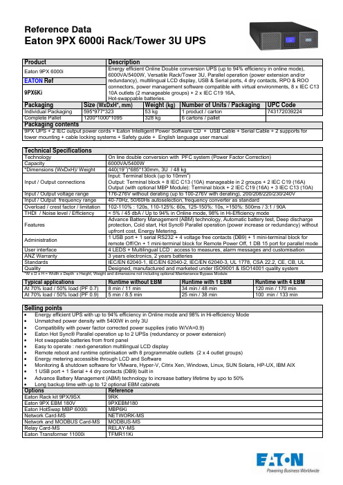
ProductDescriptionEaton 9PX 6000i Energy efficient Online Double conversion UPS (up to 94% efficiency in online mode), 6000VA/5400W, Versatile Rack/Tower 3U, Parallel operation (power extension and/or redundancy), multilingual LCD display, USB & Serial ports, 4 dry contacts, RPO & ROO connectors, power management software compatible with virtual environments, 8 x IEC C13 10A outlets (2 manageable groups) + 2 x IEC C19 16A, Hot-swappable batteries.EATON Ref 9PX6KiPackagingSize (WxDxH*, mm) Weight (kg) Number of Units / Packaging UPC Code Individual Packaging595*977*323 53 kg 1 product / carton 743172039224 Complete Pallet1200*1000*1095 328 kg 6 cartons / palletPackaging contents9PX UPS + 2 IEC output power cords + Eaton Intelligent Power Software CD + USB Cable + Serial Cable + 2 supports for tower mounting + cable locking systems + Safety guide + English language user manualTechnical SpecificationsTechnology On line double conversion with PFC system (Power Factor Correction) Capacity6000VA/5400W*Dimensions (WxDxH)/ Weight 440(19’’)*685*130mm, 3U / 48 kg Input / Output connections Input: Terminal block (up to 10mm 2)Output: Terminal block + 8 IEC C13 (10A) manageable in 2 groups + 2 IEC C19 (16A) Output (with optional MBP Module): Terminal block + 2 IEC C19 (16A) + 3 IEC C13 (10A) Input / Output voltage range 176-276V without derating (up to 100-276V with derating), 200/208/220/230/240V Input / Output frequency range 40-70Hz, 50/60Hs autoselection, frequency converter as standardOverload / crest factor / limitation 102-110% : 120s, 110-125%: 60s, 125-150%: 10s, >150%: 500ms / 3:1 / 90A THDI / Noise level / Efficiency < 5% / 45 dbA / Up to 94% in Online mode, 98% in Hi-Efficiency modeFeatures Advance Battery Management (ABM) technology, Automatic battery test, Deep discharge protection, Cold start, Hot Sync® Parallel operation (power increase or redundancy) without upfront cost, Energy Metering.Administration 1 USB port + 1 serial RS232 + 4 voltage free contacts (DB9) + 1 mini-terminal block forremote Off/On + 1 mini-terminal block for Remote Power Off, 1 DB 15 port for parallel mode User interface 4 LEDS + Multilingual LCD : access to measures, alarm messages and customisation ANZ Warranty 3 years electronics, 2 years batteriesStandards IEC/EN 62040-1, IEC/EN 62040-2, IEC/EN 62040-3, UL 1778, CSA 22.2, CE, CB, UL QualityDesigned, manufactured and marketed under ISO9001 & ISO14001 quality system *W x D x H = Width x Depth x Height, Weight and dimensions not including optional Maintenance Bypass ModuleTypical applicationsRuntime without EBM Runtime with 1 EBM Runtime with 4 EBM At 70% load / 50% load (PF 0.7) 8 min / 11 min 34 min / 48 min 120 min / 170 min At 70% load / 50% load (PF 0.9)5 min / 8.5 min25 min / 38 min100 min / 133 minSelling points∙ Energy efficient UPS with up to 94% efficiency in Online mode and 98% in Hi-efficiency Mode ∙ Unmatched power density with 5400W in only 3U∙ Compatibility with power factor corrected power supplies (ratio W/VA=0.9)∙ Eaton Hot Sync® Parallel operation up to 2 UPSs (redundancy or power extension) ∙ Hot swappable batteries from front panel∙ Easy to operate : next-generation multilingual LCD display∙ Remote reboot and runtime optimisation with 8 programmable outlets (2 x 4 outlet groups) ∙ Energy metering accessible through LCD and Software∙ Monitoring & shutdown software for VMware, Hyper-V, Citrix Xen, Windows, Linux, SUN Solaris, HP-UX, IBM AIX ∙ 1 USB port + 1 Serial + 4 dry contacts (DB9) built in∙ Advance Battery Management (ABM) technology to increase battery lifetime by upo to 50% ∙ Long backup time with up to 12 optional EBM cabinets Options Reference Eaton Rack kit 9PX/9SX 9RK Eaton 9PX EBM 180V 9PXEBM180 Eaton HotSwap MBP 6000i MBP6Ki Network Card-MS NETWORK-MS Network and MODBUS Card-MS MODBUS-MS Relay Card-MS RELAY-MS Eaton Transformer 11000i TFMR11KiProductDescriptionEaton 9PX 8000i Energy efficient Online Double conversion UPS (up to 95% efficiency in online mode), 8000VA/7200W, Versatile Rack/Tower 6U, Parallel operation (power extension and/or redundancy), multilingual LCD display, USB & Serial ports, 4 dry contacts, RPO & ROO connectors, power management software compatible with virtual environments, Hot-swappable UPS & batteries.EATON Ref9PX8KiPM + 9PXEBM240PackagingSize (WxDxH*, mm)Weight (kg) Number of Units / Packaging UPC Code PM Individual Packaging 595*977*323 24 kg 1 product / carton 743172039361 PM Complete Pallet 1200*1000*772 154kg 6 cartons / pallet EBMSee separate sheetPackaging contents PM9PX Power module + Eaton Intelligent Power Software CD + USB Cable + Serial Cable + 2 supports for tower mounting + Safety guide + English language user manual Packaging contents EBMBattery pack + 1 battery cable with comms for automatic battery cabinet recognition + link plate for tower mounting + EBM user manualTechnical SpecificationsTechnology On line double conversion with PFC system (Power Factor Correction) Capacity8000VA/7200W*Dimensions (WxDxH)/ Weight 440 (19’’)*700*260mm , 6U / 84 kgInput / Output connections Input: Terminal block (up to 16mm 2), Bypass Input: Terminal block (up to 16mm 2)Output: Terminal block (up to 16mm 2)Output (with optional MBP Module): Terminal block + 4 IEC C19 (16A)Input / Output voltage range 176-276V without derating (up to 100-276V with derating), 200/208/220/230/240/250V Input / Output frequency range 40-70Hz, 50/60Hs autoselection, frequency converter as standardOverload / crest factor / limitation 102-110% : 120s, 110-125%: 60s, 125-150%: 10s, >150%: 900ms / 3:1 / 120A THDI / Noise level / Efficiency < 5% / 48 dbA / Up to 95% in Online mode, 98% in Hi-Efficiency modeFeatures Advance Battery Management (ABM) technology, Automatic battery test, Deep discharge protection, Cold start, Hot Sync® Parallel operation (power increase or redundancy) without upfront cost, Energy Metering.Administration 1 USB port + 1 serial RS232 + 4 voltage free contacts (DB9) + 1 mini-terminal block forremote Off/On + 1 mini-terminal block for Remote Power Off, 1 DB 15 port for parallel mode User interface 4 LEDS + Multilingual LCD : access to measures, alarm messages and customisation ANZ Warranty 3 years electronics, 2 years batteriesStandards IEC/EN 62040-1, IEC/EN 62040-2, IEC/EN 62040-3, UL 1778 (Power Module), CSA 22.2, CE, CB, UL(Power Module)QualityDesigned, manufactured and marketed under ISO9001 & ISO14001 quality system *W x D x H = Width x Depth x Height, Weight and dimensions not including Maintenance BypassTypical applicationsRuntime 1 PM + 1 EBM Runtime 1 PM + 2 EBM Runtime 1 PM + 5 EBM At 70% load / 50% load (PF 0.7) 15 min / 20 min 32 min / 48 min100 min / 140 min At 70% load / 50% load (PF 0.9)10 min / 16 min25 min / 36 min75 min / 118 minSelling points∙ Energy efficient UPS with up to 95% efficiency in Online mode and 98% in Hi-efficiency Mode ∙ Compatibility with power factor corrected power supplies (ratio W/VA=0.9) ∙ UPS can be connected to 2 independant sources (AC normal , AC bypass)∙ Eaton Hot Sync® Parallel operation up to 2 UPSs (redundancy or power extension) ∙ Easy to operate : next-generation multilingual LCD display with tilt & rotation adjustment ∙ Energy metering accessible through LCD and Software∙ Monitoring & shutdown software for VMware, Hyper-V, Citrix Xen, Windows, Linux, SUN Solaris, HP-UX, IBM AIX ∙ 1 USB port + 1 Serial + 4 dry contacts (DB9) built in∙ Advance Battery Management (ABM) technology to increase battery lifetime by up to 50% ∙ Long backup time with up to 12 optional EBM cabinets Options Reference Eaton Rack kit 9PX/9SX 9RK Eaton 9PX EBM 240V 9PXEBM240 Eaton HotSwap MBP 11000i MBP11Ki Network Card-MS NETWORK-MS Network and MODBUS Card-MS MODBUS-MS Relay Card-MS RELAY-MS Eaton Supercharger 240VDC SC240RT Eaton Transformer 11000i TFMR11KiProductDescriptionEaton 9PX 11000i Energy efficient Online Double conversion UPS (up to 95% efficiency in online mode), 11000VA/10000W, Versatile Rack/Tower 6U, Internal and external Maintenance Bypass, Parallel operation (power extension and/or redundancy), multilingual LCD display, USB & Serial ports, 4 dry contacts, RPO & ROO connectors, power management software compatible with virtual environments, Hot-swappable UPS & batteries.EATON Ref9PX11KiPM + 9PXEBM240PackagingSize (WxDxH*, mm)Weight (kg) Number of Units / Packaging UPC Code PM Individual Packaging 595*977*323 26 kg 1 product / carton 743172039378 PM Complete Pallet 1200*1000*772 166kg 6 cartons / pallet EBMSee separate sheetPackaging contents PM9PX Power module + Eaton Intelligent Power Software CD + USB Cable + Serial Cable + 2 supports for tower mounting + Safety guide + English language user manual Packaging contents EBMBattery pack + 1 battery cable with comms for automatic battery cabinet recognition + link plate for tower mounting + EBM user manualTechnical SpecificationsTechnology On line double conversion with PFC system (Power Factor Correction) Capacity11000VA/10000W*Dimensions (WxDxH)/ Weight 440 (19’’)*700*260mm, 6U / 86 kgInput / Output connections Input: Terminal block (up to 16mm 2), Bypass Input: Terminal block (up to 16mm 2)Output: Terminal block (up to 16mm 2)Output (with optional MBP Module): Terminal block + 4 IEC C19 (16A)Input / Output voltage range 176-276V without derating (up to 100-276V with derating), 200/208/220/230/240/250V Input / Output frequency range 40-70Hz, 50/60Hs autoselection, frequency converter as standardOverload / crest factor / limitation 102-110% : 120s, 110-125%: 60s, 125-150%: 10s, >150%: 900ms / 3:1 / 150A THDI / Noise level / Efficiency < 5% / 50 dbA / Up to 95% in Online mode, 98% in Hi-Efficiency modeFeatures Advance Battery Management (ABM) technology, Automatic battery test, Deep discharge protection, Cold start, Hot Sync® Parallel operation (power increase or redundancy) without upfront cost, Energy Metering.Administration 1 USB port + 1 serial RS232 + 4 voltage free contacts (DB9) + 1 mini-terminal block forremote Off/On + 1 mini-terminal block for Remote Power Off, 1 DB 15 port for parallel mode User interface 4 LEDS + Multilingual LCD : access to measures, alarm messages and customisation ANZ Warranty 3 years electronics, 2 years batteriesStandards IEC/EN 62040-1, IEC/EN 62040-2, IEC/EN 62040-3, UL 1778 (Power Module), CSA 22.2, CE, CB, UL (Power Module)QualityDesigned, manufactured and marketed under ISO9001 & ISO14001 quality system *W x D x H = Width x Depth x Height, Weight and dimensions not including Maintenance BypassTypical applicationsRuntime 1 PM + 1 EBM Runtime 1 PM + 2 EBM Runtime 1 PM + 5 EBM At 70% load / 50% load (PF 0.7) 9 min / 13 min 21 min / 32 min 70 min / 100 min At 70% load / 50% load (PF 0.9)6 min / 10 min16 min / 25 min51 min / 80 minSelling points∙ Energy efficient UPS with up to 95% efficiency in Online mode and 98% in Hi-efficiency Mode ∙ Unmatched power density with 10kW in 6U∙ Compatibility with power factor corrected power supplies (ratio W/VA=0.9) ∙ UPS can be connected to 2 independant sources (AC normal , AC bypass)∙ Eaton Hot Sync® Parallel operation up to 2 UPSs (redundancy or power extension) ∙ Easy to operate : next-generation multilingual LCD display with tilt & rotation adjustment ∙ Energy metering accessible through LCD and Software∙ Monitoring & shutdown software for VMware, Hyper-V, Citrix Xen, Windows, Linux, SUN Solaris, HP-UX, IBM AIX ∙ 1 USB port + 1 Serial + 4 dry contacts (DB9) built in∙ Advance Battery Management (ABM) technology to increase battery lifetime by up to 50% ∙ Long backup time with up to 12 optional EBM cabinets Options Reference Eaton Rack kit 9PX/9SX 9RK Eaton 9PX EBM 240V 9PXEBM240 Eaton HotSwap MBP 11000i MBP11Ki Network Card-MS NETWORK-MS Network and MODBUS Card-MS MODBUS-MS Relay Card-MS RELAY-MS Eaton Supercharger 240VDC SC240RTProduct DescriptionEaton 9PX EBM 180V Extended Battery Module for 9PX 6000i RT3U, versatile Rack/Tower 3UEATON Ref9PXEBM180Packaging Size (WxDxH*, mm)Weight (kg)Number of Units / Packaging UPC CodeIndividual Packaging 595*977*323 73 kg 1 product / carton 743172039408Complete Pallet 1200*1000*1095 458 kg 6 cartons / palletPackaging contentsBattery pack + 1 battery cable with comms for automatic battery cabinet recognition + link plate for tower mounting + EBM usermanualTechnical SpecificationsDimensions (W x D x H*)/ Weight 440 (19”)*645*130 mm 3U / 68 kgANZ Warranty 2 yearsStandards IEC/EN 62040-1, IEC/EN 62040-2, IEC/EN 62040-3, CE, CB reportQuality Designed, manufactured and marketed under ISO9001 & ISO14001 quality system*W x D x H = Width x Depth x HeightRuntime in Minutes at % ofrated load (PF 0.9) 10 25 50 75 1004.53228.56000 576000 + 1 EBM 203 85 38 24 166000 + 2 EBM 399 147 71 45 286000 + 3 EBM 554 214 104 62 476000 + 4 EBM 755 287 133 90 586000 + 5 EBM 961 396 170 111 826000 + 6 EBM 1105 481 206 131 1006000 + 7 EBM >1200 542 241 156 1126000 + 8 EBM >1200 589 281 175 1266000 + 9 EBM >1200 700 331 201 1476000 + 10 EBM >1200 814 389 226 1636000 + 11 EBM >1200 908 437 251 1776000 + 12 EBM >1200 987 478 277 197Note: 4 EBMs recommended for 5/6kVA, maximum 12 EBMs possibleOptions ReferenceEaton Rack kit 9PX/9SX 9RKEaton 1,8m cable 180V EBM EBMCBL180Eaton Battery Integration System BINTSYSEaton Battery Cable Adaptor for MX/9135 CBLADAPT180Product DescriptionEaton 9PX EBM 240VBattery Extension cabinet for 9PX 8000/11000i, versatile Rack/Tower 3UEATON Ref9PXEBM240Packaging Size (WxDxH*, mm)Weight (kg)Number of Units / Packaging UPC Code Individual Packaging 595*977*323 70 kg 1 product / carton 743172039422 Complete Pallet 1200*1000*1095 440 kg 6 cartons / palletPackaging contentsBattery pack + 1 battery cable with comms for automatic battery cabinet recognition + link plate for tower mounting + EBM user manualTechnical SpecificationsDimensions (W x D x H*)/ Weight 440 (19”)*680*130 mm 3U / 65 kgANZ Warranty 2 yearsStandards IEC/EN 62040-1, IEC/EN 62040-2, IEC/EN 62040-3, CE, CB reportQuality Designed, manufactured and marketed under ISO9001 & ISO14001 quality system*W x D x H = Width x Depth x HeightRuntime in Minutes at % of10 25 50 75 100 rated load (PF 0.9)8K Std (1PM + 1EBM) 106 35 16 9 58K Std + 1 EBM 203 85 36 23 168K Std + 2 EBM 342 140 65 36 278K Std + 3 EBM 492 173 86 53 368K Std + 4 EBM 582 220 118 72 508K Std + 5 EBM 748 272 143 86 658K Std + 6 EBM 898 341 162 109 768K Std + 7 EBM 1011 416 175 127 868K Std + 8 EBM 1099 475 199 143 1038K Std + 9 EBM 1168 522 225 156 1188K Std + 10 EBM >1200 560 250 167 1318K Std + 11 EBM >1200 591 279 175 143Runtime in Minutes at % of10 25 50 75 100 rated load (PF 0.9)11K Std (1PM + 1EBM) 74 25 10 5.5 311K Std + 1 EBM 159 60 25 15 1011K Std + 2 EBM 237 97 42 25 1811K Std + 3 EBM 341 136 61 37 2511K Std + 4 EBM 461 163 80 48 3411K Std + 5 EBM 541 184 98 61 4211K Std + 6 EBM 598 223 120 73 5111K Std + 7 EBM 747 261 139 86 6111K Std + 8 EBM 864 298 153 98 6911K Std + 9 EBM 957 361 165 113 7911K Std + 10 EBM 1033 414 175 127 8911K Std + 11 EBM 1098 458 190 139 98 Note: 6 EBMs recommended for 8/11kVA, maximum 12 EBMs (or 400Ah) possible with additional charger (Supercharger option) Options ReferenceEaton Rack kit 9PX/9SX 9RKEaton 1,8m cable 240V EBM EBMCBL240Eaton Battery Integration System BINTSYSEaton Battery Cable Adaptor for EXRT CBLADAPT240。
基于链间耦合的并联悬架的刚度优化

基于链间耦合的并联悬架的刚度优化贾登峰万小金(武汉理工大学汽车工程学院汽车零部件先进技术湖北省重点实验室,湖北武汉430070)摘要针对越野车辆座椅刚度提升问题,提出了利用并联机构作为座椅悬架主体结构的方案。
为保证悬架装置具有高精度位姿和高刚度结构,对链间耦合与固有频率进行研究。
首先,通过能量法、虚功原理和扰动理论,可以获得机构的广义质量和广义刚度矩阵;其次,弹性耦合和惯性耦合是基于以上两个广义矩阵而定义的两个指标来测量并联机构的耦合程度,通过Cholesky分解法获得机构的固有频率;然后,为了获得较小的弹性耦合、惯性耦合和较大的固有频率,以固有频率作为目标函数来优化悬架装置的结构参数;最终,对优化结果综合分析,获得最优结构参数用于改进装置结构。
关键词并联悬架固有频率弹性耦合与惯性耦合刚度优化Stiffness Optimization of Parallel Suspension based on Inter-chain CouplingJia Dengfeng Wan Xiaojin(Hubei Key Laboratory of Advanced Technology for Automotive Components,School of Automotive Engineering,Wuhan University of Technology,Wuhan430070,China)Abstract For the improvement of off-road vehicle seat stiffness,a scheme of using parallel mechanism as the main structure of the seat suspension is proposed.The coupling between chains and the natural frequen‐cy are studied to ensure that the suspension mechanism has high precision and high stiffness.Firstly,general‐ized mass and generalized stiffness matrices of the mechanism can be obtained by means of energy method,vir‐tual work principle and disturbance theory.Secondly,elastic coupling and inertial coupling are two indexes de‐fined based on the above two generalized matrices to measure the coupling degree of the parallel mechanism. Cholesky decomposition method is used to obtain the natural frequency of the mechanism.Then,in order to ob‐tain the small elastic coupling,the inertial coupling and a large natural frequency,the natural frequency is used as the objective function to optimize the structural parameters of the suspension mechanism.Finally,the optimization results are comprehensively analyzed and the optimal structural parameters are obtained to im‐prove the structure of the device.Key words Parallel suspension Natural frequency Inertial coupling and elastic coupling Stiffness optimization0引言越野车辆由于工作环境恶劣,有众多激励振源。
国际计算机会议与期刊分级列表
Computer Science Department Conference RankingsSome conferences accept multiple categories of papers. The rankingsbelow are for the most prestigious category of paper at a givenconference. All other categories should be treated as "unranked".AREA: Artificial Intelligence and Related SubjectsRank 1:IJCAI: Intl Joint Conf on AIAAAI: American Association for AI National ConferenceICAA: International Conference on Autonomous Agents(现改名为AAMAS) CVPR: IEEE Conf on Comp Vision and Pattern RecognitionICCV: Intl Conf on Computer VisionICML: Intl Conf on Machine LearningKDD: Knowledge Discovery and Data MiningKR: Intl Conf on Principles of KR & ReasoningNIPS: Neural Information Processing SystemsUAI: Conference on Uncertainty in AIACL: Annual Meeting of the ACL (Association of Computational Linguistics) Rank 2:AID: Intl Conf on AI in DesignAI-ED: World Conference on AI in EducationCAIP: Inttl Conf on Comp. Analysis of Images and PatternsCSSAC: Cognitive Science Society Annual ConferenceECCV: European Conference on Computer VisionEAI: European Conf on AIEML: European Conf on Machine LearningGP: Genetic Programming ConferenceIAAI: Innovative Applications in AIICIP: Intl Conf on Image ProcessingICNN/IJCNN: Intl (Joint) Conference on Neural NetworksICPR: Intl Conf on Pattern RecognitionICDAR: International Conference on Document Analysis and RecognitionICTAI: IEEE conference on Tools with AIAMAI: Artificial Intelligence and MathsDAS: International Workshop on Document Analysis SystemsWACV: IEEE Workshop on Apps of Computer VisionCOLING: International Conference on Computational LiguisticsEMNLP: Empirical Methods in Natural Language ProcessingRank 3:PRICAI: Pacific Rim Intl Conf on AIAAI: Australian National Conf on AIACCV: Asian Conference on Computer VisionAI*IA: Congress of the Italian Assoc for AIANNIE: Artificial Neural Networks in EngineeringANZIIS: Australian/NZ Conf on Intelligent Inf. SystemsCAIA: Conf on AI for ApplicationsCAAI: Canadian Artificial Intelligence ConferenceASADM: Chicago ASA Data Mining Conf: A Hard Look at DMEPIA: Portuguese Conference on Artificial IntelligenceFCKAML: French Conf on Know. Acquisition & Machine LearningICANN: International Conf on Artificial Neural NetworksICCB: International Conference on Case-Based ReasoningICGA: International Conference on Genetic AlgorithmsICONIP: Intl Conf on Neural Information ProcessingIEA/AIE: Intl Conf on Ind. & Eng. Apps of AI & Expert SysICMS: International Conference on Multiagent SystemsICPS: International conference on Planning SystemsIWANN: Intl Work-Conf on Art & Natural Neural NetworksPACES: Pacific Asian Conference on Expert SystemsSCAI: Scandinavian Conference on Artifical IntelligenceSPICIS: Singapore Intl Conf on Intelligent SystemPAKDD: Pacific-Asia Conf on Know. Discovery & Data MiningSMC: IEEE Intl Conf on Systems, Man and CyberneticsPAKDDM: Practical App of Knowledge Discovery & Data MiningWCNN: The World Congress on Neural NetworksWCES: World Congress on Expert SystemsINBS: IEEE Intl Symp on Intell. in Neural \& Bio SystemsASC: Intl Conf on AI and Soft ComputingPACLIC: Pacific Asia Conference on Language, Information and Computation ICCC: International Conference on Chinese ComputingOthers:ICRA: IEEE Intl Conf on Robotics and AutomationNNSP: Neural Networks for Signal ProcessingICASSP: IEEE Intl Conf on Acoustics, Speech and SPGCCCE: Global Chinese Conference on Computers in EducationICAI: Intl Conf on Artificial IntelligenceAEN: IASTED Intl Conf on AI, Exp Sys & Neural NetworksWMSCI: World Multiconfs on Sys, Cybernetics & InformaticsAREA: Hardware and ArchitectureRank 1:ASPLOS: Architectural Support for Prog Lang and OSISCA: ACM/IEEE Symp on Computer ArchitectureICCAD: Intl Conf on Computer-Aided DesignDAC: Design Automation ConfMICRO: Intl Symp on MicroarchitectureHPCA: IEEE Symp on High-Perf Comp ArchitectureRank 2:FCCM: IEEE Symposium on Field Programmable Custom Computing Machines SUPER: ACM/IEEE Supercomputing ConferenceICS: Intl Conf on SupercomputingISSCC: IEEE Intl Solid-State Circuits ConfHCS: Hot Chips SympVLSI: IEEE Symp VLSI CircuitsISSS: International Symposium on System SynthesisDATE: IEEE/ACM Design, Automation & Test in Europe ConferenceRank 3:ICA3PP: Algs and Archs for Parall ProcEuroMICRO: New Frontiers of Information TechnologyACS: Australian Supercomputing ConfUnranked:Advanced Research in VLSIInternational Symposium on System SynthesisInternational Symposium on Computer DesignInternational Symposium on Circuits and SystemsAsia Pacific Design Automation ConferenceInternational Symposium on Physical DesignInternational Conference on VLSI DesignAREA: ApplicationsRank 1:I3DG: ACM-SIGRAPH Interactive 3D GraphicsSIGGRAPH: ACM SIGGRAPH ConferenceACM-MM: ACM Multimedia ConferenceDCC: Data Compression ConfSIGMETRICS: ACM Conf on Meas. & Modelling of Comp SysSIGIR: ACM SIGIR Conf on Information RetrievalPECCS: IFIP Intl Conf on Perf Eval of Comp \& Comm SysWWW: World-Wide Web ConferenceRank 2:EUROGRAPH: European Graphics ConferenceCGI: Computer Graphics InternationalCANIM: Computer AnimationPG: Pacific GraphicsIEEE-MM: IEEE Intl Conf on Multimedia Computing and SysNOSSDAV: Network and OS Support for Digital A/VPADS: ACM/IEEE/SCS Workshop on Parallel \& Dist Simulation WSC: Winter Simulation ConferenceASS: IEEE Annual Simulation SymposiumMASCOTS: Symp Model Analysis \& Sim of Comp \& Telecom Sys PT: Perf Tools - Intl Conf on Model Tech \& Tools for CPENetStore - Network Storage SymposiumRank 3:ACM-HPC: ACM Hypertext ConfMMM: Multimedia ModellingDSS: Distributed Simulation SymposiumSCSC: Summer Computer Simulation ConferenceWCSS: World Congress on Systems SimulationESS: European Simulation SymposiumESM: European Simulation MulticonferenceHPCN: High-Performance Computing and NetworkingGeometry Modeling and ProcessingWISEDS-RT: Distributed Simulation and Real-time ApplicationsIEEE Intl Wshop on Dist Int Simul and Real-Time ApplicationsUn-ranked:DVAT: IS\&T/SPIE Conf on Dig Video Compression Alg \& Tech MME: IEEE Intl Conf. on Multimedia in EducationICMSO: Intl Conf on Modelling, Simulation and OptimisationICMS: IASTED Intl Conf on Modelling and SimulationAREA: System TechnologyRank 1:SIGCOMM: ACM Conf on Comm Architectures, Protocols & Apps INFOCOM: Annual Joint Conf IEEE Comp & Comm SocSPAA: Symp on Parallel Algms and ArchitecturePODC: ACM Symp on Principles of Distributed ComputingPPoPP: Principles and Practice of Parallel ProgrammingMassPar: Symp on Frontiers of Massively Parallel ProcRTSS: Real Time Systems SympSOSP: ACM SIGOPS Symp on OS PrinciplesSOSDI: Usenix Symp on OS Design and ImplementationCCS: ACM Conf on Comp and Communications SecurityIEEE Symposium on Security and PrivacyMOBICOM: ACM Intl Conf on Mobile Computing and Networking USENIX Conf on Internet Tech and SysICNP: Intl Conf on Network ProtocolsOPENARCH: IEEE Conf on Open Arch and Network ProgPACT: Intl Conf on Parallel Arch and Compil TechRank 2:CC: Compiler ConstructionIPDPS: Intl Parallel and Dist Processing SympIC3N: Intl Conf on Comp Comm and NetworksICPP: Intl Conf on Parallel ProcessingICDCS: IEEE Intl Conf on Distributed Comp SystemsSRDS: Symp on Reliable Distributed SystemsMPPOI: Massively Par Proc Using Opt InterconnsASAP: Intl Conf on Apps for Specific Array ProcessorsEuro-Par: European Conf. on Parallel ComputingFast Software EncryptionUsenix Security SymposiumEuropean Symposium on Research in Computer SecurityWCW: Web Caching WorkshopLCN: IEEE Annual Conference on Local Computer NetworksIPCCC: IEEE Intl Phoenix Conf on Comp & CommunicationsCCC: Cluster Computing ConferenceICC: Intl Conf on CommRank 3:MPCS: Intl. Conf. on Massively Parallel Computing SystemsGLOBECOM: Global CommICCC: Intl Conf on Comp CommunicationNOMS: IEEE Network Operations and Management SympCONPAR: Intl Conf on Vector and Parallel ProcessingVAPP: Vector and Parallel ProcessingICPADS: Intl Conf. on Parallel and Distributed SystemsPublic Key CryptosystemsIEEE Computer Security Foundations WorkshopAnnual Workshop on Selected Areas in CryptographyAustralasia Conference on Information Security and PrivacyInt. Conf on Inofrm and Comm. SecurityFinancial CryptographyWorkshop on Information HidingSmart Card Research and Advanced Application ConferenceICON: Intl Conf on NetworksIMSA: Intl Conf on Internet and MMedia SysNCC: Nat Conf CommIN: IEEE Intell Network WorkshopICME: Intl Conf on MMedia & ExpoSoftcomm: Conf on Software in Tcomms and Comp NetworksINET: Internet Society ConfWorkshop on Security and Privacy in E-commerceUn-ranked:PARCO: Parallel ComputingSE: Intl Conf on Systems EngineeringAREA: Programming Languages and Software EngineeringRank 1:POPL: ACM-SIGACT Symp on Principles of Prog LangsPLDI: ACM-SIGPLAN Symp on Prog Lang Design & ImplOOPSLA: OO Prog Systems, Langs and ApplicationsICFP: Intl Conf on Function ProgrammingJICSLP/ICLP/ILPS: (Joint) Intl Conf/Symp on Logic ProgICSE: Intl Conf on Software EngineeringFSE: ACM Conference on the Foundations of Software Engineering (inc: ESEC-FSE when held jointly)FM/FME: Formal Methods, World Congress/EuropeCAV: Computer Aided VerificationRank 2:CP: Intl Conf on Principles & Practice of Constraint ProgTACAS: Tools and Algos for the Const and An of SystemsESOP: European Conf on ProgrammingICCL: IEEE Intl Conf on Computer LanguagesPEPM: Symp on Partial Evalutation and Prog ManipulationSAS: Static Analysis SymposiumRTA: Rewriting Techniques and ApplicationsESEC: European Software Engineering ConfIWSSD: Intl Workshop on S/W Spec & DesignCAiSE: Intl Conf on Advanced Info System EngineeringITC: IEEE Intl Test ConfIWCASE: Intl Workshop on Cumpter-Aided Software EngSSR: ACM SIGSOFT Working Conf on Software ReusabilitySEKE: Intl Conf on S/E and Knowledge EngineeringICSR: IEEE Intl Conf on Software ReuseASE: Automated Software Engineering ConferencePADL: Practical Aspects of Declarative LanguagesISRE: Requirements EngineeringICECCS: IEEE Intl Conf on Eng. of Complex Computer SystemsIEEE Intl Conf on Formal Engineering MethodsIntl Conf on Integrated Formal MethodsFOSSACS: Foundations of Software Science and Comp StructRank 3:FASE: Fund Appr to Soft EngAPSEC: Asia-Pacific S/E ConfPAP/PACT: Practical Aspects of PROLOG/Constraint TechALP: Intl Conf on Algebraic and Logic ProgrammingPLILP: Prog, Lang Implentation & Logic ProgrammingLOPSTR: Intl Workshop on Logic Prog Synthesis & TransfICCC: Intl Conf on Compiler ConstructionCOMPSAC: Intl. Computer S/W and Applications ConfCSM: Conf on Software MaintenanceTAPSOFT: Intl Joint Conf on Theory & Pract of S/W DevWCRE: SIGSOFT Working Conf on Reverse EngineeringAQSDT: Symp on Assessment of Quality S/W Dev ToolsIFIP Intl Conf on Open Distributed ProcessingIntl Conf of Z UsersIFIP Joint Int'l Conference on Formal Description Techniques and Protocol Specification, Testing, And VerificationPSI (Ershov conference)UML: International Conference on the Unified Modeling LanguageUn-ranked:Australian Software Engineering ConferenceIEEE Int. W'shop on Object-oriented Real-time Dependable Sys. (WORDS)IEEE International Symposium on High Assurance Systems EngineeringThe Northern Formal Methods WorkshopsFormal Methods PacificInt. Workshop on Formal Methods for Industrial Critical SystemsJFPLC - International French Speaking Conference on Logic and Constraint ProgrammingL&L - Workshop on Logic and LearningSFP - Scottish Functional Programming WorkshopHASKELL - Haskell WorkshopLCCS - International Workshop on Logic and Complexity in Computer ScienceVLFM - Visual Languages and Formal MethodsNASA LaRC Formal Methods Workshop(1) FATES - A Satellite workshop on Formal Approaches to Testing of Software(1) Workshop On Java For High-Performance Computing(1) DSLSE - Domain-Specific Languages for Software Engineering(1) FTJP - Workshop on Formal Techniques for Java Programs(*) WFLP - International Workshop on Functional and (Constraint) Logic Programming(*) FOOL - International Workshop on Foundations of Object-Oriented Languages(*) SREIS - Symposium on Requirements Engineering for Information Security(*) HLPP - International workshop on High-level parallel programming and applications(*) INAP - International Conference on Applications of Prolog(*) MPOOL - Workshop on Multiparadigm Programming with OO Languages(*) PADO - Symposium on Programs as Data Objects(*) TOOLS: Int'l Conf Technology of Object-Oriented Languages and Systems(*) Australasian Conference on Parallel And Real-Time SystemsAREA: Algorithms and TheoryRank 1:STOC: ACM Symp on Theory of ComputingFOCS: IEEE Symp on Foundations of Computer ScienceCOLT: Computational Learning TheoryLICS: IEEE Symp on Logic in Computer ScienceSCG: ACM Symp on Computational GeometrySODA: ACM/SIAM Symp on Discrete AlgorithmsSPAA: ACM Symp on Parallel Algorithms and ArchitecturesPODC: ACM Symp on Principles of Distributed ComputingISSAC: Intl. Symp on Symbolic and Algebraic ComputationCRYPTO: Advances in CryptologyEUROCRYPT: European Conf on CryptographyRank 2:CONCUR: International Conference on Concurrency TheoryICALP: Intl Colloquium on Automata, Languages and ProgSTACS: Symp on Theoretical Aspects of Computer ScienceCC: IEEE Symp on Computational ComplexityWADS: Workshop on Algorithms and Data StructuresMFCS: Mathematical Foundations of Computer ScienceSWAT: Scandinavian Workshop on Algorithm TheoryESA: European Symp on AlgorithmsIPCO: MPS Conf on integer programming & comb optimization LFCS: Logical Foundations of Computer ScienceALT: Algorithmic Learning TheoryEUROCOLT: European Conf on Learning TheoryWDAG: Workshop on Distributed AlgorithmsISTCS: Israel Symp on Theory of Computing and SystemsISAAC: Intl Symp on Algorithms and ComputationFST&TCS: Foundations of S/W Tech & Theoretical CSLATIN: Intl Symp on Latin American Theoretical InformaticsRECOMB: Annual Intl Conf on Comp Molecular BiologyCADE: Conf on Automated DeductionIEEEIT: IEEE Symposium on Information TheoryAsiacryptRank 3:MEGA: Methods Effectives en Geometrie AlgebriqueASIAN: Asian Computing Science ConfCCCG: Canadian Conf on Computational GeometryFCT: Fundamentals of Computation TheoryWG: Workshop on Graph TheoryCIAC: Italian Conf on Algorithms and ComplexityICCI: Advances in Computing and InformationAWTI: Argentine Workshop on Theoretical InformaticsCATS: The Australian Theory SympCOCOON: Annual Intl Computing and Combinatorics ConfUMC: Unconventional Models of ComputationMCU: Universal Machines and ComputationsGD: Graph DrawingSIROCCO: Structural Info & Communication ComplexityALEX: Algorithms and ExperimentsALG: ENGG Workshop on Algorithm EngineeringLPMA: Intl Workshop on Logic Programming and Multi-Agents EWLR: European Workshop on Learning RobotsCITB: Complexity & info-theoretic approaches to biologyFTP: Intl Workshop on First-Order Theorem Proving (FTP)CSL: Annual Conf on Computer Science Logic (CSL)AAAAECC: Conf On Applied Algebra, Algebraic Algms & ECC DMTCS: Intl Conf on Disc Math and TCSUn-ranked:Information Theory WorkshopAREA: Data BasesRank 1:SIGMOD: ACM SIGMOD Conf on Management of DataPODS: ACM SIGMOD Conf on Principles of DB SystemsVLDB: Very Large Data BasesICDE: Intl Conf on Data EngineeringICDT: Intl Conf on Database TheoryRank 2:SSD: Intl Symp on Large Spatial DatabasesDEXA: Database and Expert System ApplicationsFODO: Intl Conf on Foundation on Data OrganizationEDBT: Extending DB TechnologyDOOD: Deductive and Object-Oriented DatabasesDASFAA: Database Systems for Advanced ApplicationsCIKM: Intl. Conf on Information and Knowledge ManagementSSDBM: Intl Conf on Scientific and Statistical DB MgmtCoopIS - Conference on Cooperative Information SystemsER - Intl Conf on Conceptual Modeling (ER)Rank 3:COMAD: Intl Conf on Management of DataBNCOD: British National Conference on DatabasesADC: Australasian Database ConferenceADBIS: Symposium on Advances in DB and Information SystemsDaWaK - Data Warehousing and Knowledge DiscoveryRIDE WorkshopIFIP-DS: IFIP-DS ConferenceIFIP-DBSEC - IFIP Workshop on Database SecurityNGDB: Intl Symp on Next Generation DB Systems and AppsADTI: Intl Symp on Advanced DB Technologies and IntegrationFEWFDB: Far East Workshop on Future DB SystemsMDM - Int. Conf. on Mobile Data Access/Management (MDA/MDM)ICDM - IEEE International Conference on Data MiningVDB - Visual Database SystemsIDEAS - International Database Engineering and Application SymposiumOthers:ARTDB - Active and Real-Time Database SystemsCODAS: Intl Symp on Cooperative DB Systems for Adv AppsDBPL - Workshop on Database Programming LanguagesEFIS/EFDBS - Engineering Federated Information (Database) SystemsKRDB - Knowledge Representation Meets DatabasesNDB - National Database Conference (China)NLDB - Applications of Natural Language to Data BasesKDDMBD - Knowledge Discovery and Data Mining in Biological Databases Meeting FQAS - Flexible Query-Answering SystemsIDC(W) - International Database Conference (HK CS)RTDB - Workshop on Real-Time DatabasesSBBD: Brazilian Symposium on DatabasesWebDB - International Workshop on the Web and DatabasesWAIM: Interational Conference on Web Age Information Management(1) DASWIS - Data Semantics in Web Information Systems(1) DMDW - Design and Management of Data Warehouses(1) DOLAP - International Workshop on Data Warehousing and OLAP(1) DMKD - Workshop on Research Issues in Data Mining and Knowledge Discovery (1) KDEX - Knowledge and Data Engineering Exchange Workshop(1) NRDM - Workshop on Network-Related Data Management(1) MobiDE - Workshop on Data Engineering for Wireless and Mobile Access(1) MDDS - Mobility in Databases and Distributed Systems(1) MEWS - Mining for Enhanced Web Search(1) TAKMA - Theory and Applications of Knowledge MAnagement(1) WIDM: International Workshop on Web Information and Data Management(1) W2GIS - International Workshop on Web and Wireless Geographical Information Systems * CDB - Constraint Databases and Applications* DTVE - Workshop on Database Technology for Virtual Enterprises* IWDOM - International Workshop on Distributed Object Management* IW-MMDBMS - Int. Workshop on Multi-Media Data Base Management Systems* OODBS - Workshop on Object-Oriented Database Systems* PDIS: Parallel and Distributed Information SystemsAREA: MiscellaneousRank 1:Rank 2:AMIA: American Medical Informatics Annual Fall SymposiumDNA: Meeting on DNA Based ComputersRank 3:MEDINFO: World Congress on Medical InformaticsInternational Conference on Sequences and their ApplicationsECAIM: European Conf on AI in MedicineAPAMI: Asia Pacific Assoc for Medical Informatics ConfSAC: ACM/SIGAPP Symposium on Applied ComputingICSC: Internal Computer Science ConferenceISCIS: Intl Symp on Computer and Information SciencesICSC2: International Computer Symposium ConferenceICCE: Intl Conf on Comps in EduEd-MediaWCC: World Computing CongressPATAT: Practice and Theory of Automated TimetablingNot Encouraged (due to dubious referee process):International Multiconferences in Computer Science -- 14 joint int'l confs.SCI: World Multi confs on systemics, sybernetics and informaticsSSGRR: International conf on Advances in Infrastructure for e-B, e-Edu and e-Science and e-MedicineIASTED conferences以下是期刊:IEEE/ACM TRANSACTIONS期刊系列一般都被公认为领域顶级期刊,所以以下列表在关于IEEE/ACM TRANSACTIONS的分类不一定太准确。
ABBYY FineReader Engine性能指南
ABBYY FineReader EnginePerformance GuideIntegrating optical character recognition (OCR) technology will effectively extend the functionality of your application.Excellent performance of the OCR component is one of the key factors for high customer satisfaction.This document provides information on general OCR performance factors and the possibilities to optimize them in the Software Development Kit ABBYY FineReader Engine. By utilizing its advanced capabilities and options, the high OCR performance can be improved even further for optimal customer experience.When measuring OCR performance, there are two major parameters to consider:RECOGNITION ACCURACYPROCESSING SPEEDWhich Factors Influence the OCR Accuracyand Processing Speed?Image Type and Image QualityImages can come from different sources. Digitally createdPDFs, screenshots of computer and tablet devices, imagefiles created by scanners, fax servers, digital camerasor smartphones – various image sources will lead todifferent image types with different level of image quality.For example, using the wrong scanner settings can cause“noise” on the image, like random black dots or speckles,blurred and uneven letters, or skewed lines and shiftedtable borders. In terms of OCR, this is a ‘low-qualityimage’.Processing low-quality images requires high computingpower, increases the overall processing time and deterio-rates the recognition results.On the other hand, processing ‘high-quality images’ with-out distortions reduces the processing time. A dditionally,reading high-quality images leads to higher accuracyresults.Therefore, it is recommended to use high-quality imagesfor the OCR process.If it is not possible to influence the image quality in advance, it is recommended to enhance it prior to the recognition step. In FineReader Engine, various powerful image preprocessing functions are available:it is possible to use automatic language detection., a high number of preselected recognition languagesTo increase the recognition accuracy even more, FineReaderEngine provides dictionary and morphology support formany languages. When processing documents includingsubject-specific terms or …structures“ such as productcodes, telephone numbers or passport numbers, customcreated dictionaries can be imported to ensure high recog-nition quality.AAfrom a scanner or imported from the storage system or the memory stream. To obtain images from different sources will require different methods and influence the recognition speed. The image import from memory is generally faster than opening the images from a file storage.Image PreprocessingGenerally, the OCR process is faster for good-quality images. It is recommended to fine-tune the image preprocessing step accordingly and therefore savetime during the actual processing step.Images can be of different formats and quality. High-quality images, such as digitally created PDFs, typically do not require a lot of preprocessing work. For low-quality images, like scanned documents with incorrect scanner settings or old books, it is necessary to apply advanced imagepreprocessing functions to improve the recognition results. For the preprocessing of digital photos, the special ABBYYC amera OCR™ technology is applied. Here, the algorithms are optimized specifically for photo e nhancement. Usage of different preprocessing functions will individually influence the processing speed.The different methods and parameters used for specific processing scenarios will significantly influence the overall processing speed. Discarding unnecessary stages can speed up the entire OCR process. For example, when extracting data from predefined document areas, the document analysis is not required. When exporting the documents to TXT format or to PDF Image Only format, the synthesis stage can be skipped.Document AnalysisBrochures or newspapers often contain text in columns, tables, diagrams and pictures. Technical drawings might be large documents including complex engineering diagrams with different text orientation. For documents with such compli-cated layouts, the document analysis step will require more processing time. On the other hand, the analysis of simplelayout document like letters or contracts is very fast.Parallel Processing Using Multiple CoresFineReader Engine can be used to build applications of any scale and complexity – from a client workstation to a server- based solution or a large multi-million page project. When it comes to the OCR performance, it often makes sense to utilize multi-processor or multi-core systems to increase the processing speed.Built-in multi-core support in FineReader Engine allows different approaches to scale-up the OCR process:• Utilizing a single Engine instance• Loading several Engine instancesThere are different approaches for processing documents:Processing of Large Multi-Page DocumentsFor parallel processing of large documents with many pages the ‘FRDocument’ object is best suited. In this case, the pages of a multi-page document are processed in parallel on the CPUs available. At the end, the results are combined into one multi-page document. It is the most easy-to-code multiprocessing way. The number of processes needed is detected automatically, depending on factors such as the number of available physical or logical CPU cores, the number of free CPU cores available in the license, and the number of pages in the document. If nec-essary, the developer can easily change the multiprocess-ing settings and tune the number of processes to be run.Processing of Many Single-Page DocumentsTo process many one-page documents in parallel, which are received from the same source, e.g. a scanner, it is recommended to use the ‘BatchProcessor’ object. This object is most effective in terms of speed, when document export is not required, like in data capture scenarios with a custom output format.To perform full processing of many one-page documentsin parallel, it is recommended to use a pool of Engine in-stances. This approach is also best suited for web-service scenarios, when the input document should be processed directly after it was submitted. In this case, the document is passed to an available FineReader Engine instance from the pool and processed immediately.FineReader Engine - Speed Testing ResultsSystem ResourcesThe table presents the results of internal performance testing. Please be aware that testing results always depend on many factors, such as image quality, used recognition languages and other factors.During the OCR process, a range of different algorithms are applied. They depend on image quality, document languages, layout complexity and number of pages in the document. Accordingly, such algorithms might require higher memory resources. It is recommended to set up the system in accordance with the outlined memory requirements to optimize the processing speed by allocating adequate system memory.Technical Test InformationIntel® Core™ i5-4440 (3.10 GHz, 4 physical cores), 8 GB RAM, 4 processes running simultaneously.The performance was tested on 300 documents in E nglish, using the ‘DocumentArchiving_Speed’ predefined profile. In thescenarios …One-page d ocuments“ and …One multi-page d ocument“ the d ocuments were exported as PDF format.* The text was extracted from pre-defined areas on one-page documents. No export to any file format was performed.How to Increase the Overall Processing Speed in FineReader EngineHow to Improve the Text Recognition Quality in FineReader EngineThere are several possibilities to improve the performance of your system:• Fine-tune the image preprocessing settings to deliver the highest document quality for the processing step.• During the processing step, use one of the predefined processing profiles optimized for speed and the appropriate recognition mode – balanced or fast.• Specify the correct recognition languages. Incorrect language can significantly slow down document processing. The more recognition languages are selected, the slower the speed of processing. • Use the appropriate object (FRDocument or BatchProcessor) and enable parallel processing.• Specify appropriate parameters of analysis and recognition. For example, disable table detection and page orientation correction if images contain no tables and have correct page orientation.• Omit the synthesis stage if the processed documents will be exported to TXT format or PDF Image Only format.• Use the Fast PDF Export Profile, when exporting the documents to the PDF format.• Use the special object (ExportFileWriter), which is designed for the export of very large multi-page documents into PDF format.For more information, refer to the FineReader Engine Developer’s Help:FineReader Engine offers high recognition quality. The recognition quality will always depend on factors such as image quality, language and other factors. However, there are several ways to increase the recognition quality:• Specify the correct text type.• Specify the appropriate recognition languages.• Define unique languages and custom dictionaries for the recognition of special characters or documents with specific terminology, e.g. legal or healthcare texts.• Split the facing pages of scanned books into two separate images.• Apply the special Camera OCR technology, when digital photos are processed.• Correct resolution of the image, if it significantly differs from the recommended resolution.For more information refer to the FineReader Engine Developer’s Help:As you know, in document processing the OCR process can be a very complex task. Depending on the individual document processing scenario, the OCR performance results can significantly vary. The tips for recognition accuracy and processing speed optimisation in ABBYY FineReader Engine should help you to achieve the optimal performance for your business case.Additional Information ResourcesIndividual Project SupportTo learn more about the different aspects of OCR performance optimisation and about the SDK ABBYY FineReader Engine, please use following sources of information:• ABBYY Technology portal: https://abbyy.technology/• ABBYY OCR SDK forum: https:///• The help file provided in the ABBYY FineReader Engine distributive • ABBYY FineReader Engine product pages on /ocr-sdk .If you would like to discuss a particular project, please contact us. During the testing period, you can ask standard technical questions to our ABBYY Technical Support or use ABBYY Professional Services foradvanced consultancy, in-depth project analysis and individual code review. Using ABBYY’s technical resources can shorten your development work and speed up your project. Please contact the ABBYY sales manager, if you wish to further explore these options.If you have additional questions, contact your local ABBYY representative listed under /contacts or use the online contact form /ocr-sdk/#request-demo .This software includes ABBYY® FineReader® Engine 12 recognition technologies. © 2017, ABBYY Production LLC. ABBYY , FINEREADER and ABBYY FineReader are either registered trademarks or trademarks of ABBYY Software Ltd. All product names, trademarks and registered trademarks are property of their respective owners. Windows® is a registered trademark of Microsoft Corporation in the United States and other countries. The registered trademark Linux® is used pursuant to a sublicense from LMI, the exclusive licensee of Linus Torvalds, owner of the mark on a world-wide basis. Mac® and OS X® are trademarks of Apple Inc., registered in the U.S. and other countries. Datalogics®, The DL Logo®, PDF2IMG™ and DLE™ are trademarks of Datalogics, Inc. Adobe®, The Adobe Logo®, Adobe® PDF Library™, Powered by Adobe PDF Library logo, Reader® are either registered trademarks or trademarks of Adobe Systems Incorporated in the United States and/or other countries. Portions of this computer program are copyright © 1996-2007 LizardTech, Inc. The software is based in part on the work of the Independent JPEG Group. Portions of this software are copyright ©2011 University of New South Wales. Unicode support: © 1991-2013 Unicode, Inc. Intel® Performance Primitives: Copyright © 2002-2008 Intel Corporation. Portions of this software are copyright © 1996-2002, 2006 The FreeType Project . WIBU, CodeMeter, SmartShelter, and SmartBind are registered trademarks of Wibu-Systems. All rights reserved. All other trademarks are the property of their respective owners. #9612en。
Automated optimal design of mechanical conformational switches
1
Artificial Life 2(2):129–156, 1995.
2
(a)
enzyme
substrate conformational change
enzyme-substrate complex
(b)
Hale Waihona Puke end-product inhibitor
enzyme
substrate
inactive enzyme
Saitou, K., Jakiela, M. J., “Automated Optimal Design of Mechanical Conformational Switches,” Artificial Life 2(2):129–156, 1995.
Automated Optimal Design of Mechanical Conformational Switches
Kazuhiro Saitou Mark J. Jakiela Computer-Aided Design Laboratory Massachusetts Institute of Technology
∗
Abstract Bacteriophage viruses spontaneously self-assemble in the presence of their component parts (certain protein molecules). It is believed that conformational switches, interacting chemical bonding sites that allow tentative incorrect bonds, facilitate this randomized assembly process. A onedimensional conformational switch is proposed and used to study the randomized assembly of mechanical parts. A genetic algorithm is used to search the space of parameterized switch designs to maximize the rate of a desired assembly. Keywords: randomized assembly, mechanical conformational switches, genetic optimization
英文原文
International Journal of Vehicle Design,Vol. 26, Nos. 2/3, 2001, pp. 264-276.Sliding Mode Control of Active Suspensions for a Full Vehicle Model N.YAGIZ* and I.YUKSEK***Department of Mechanical Engineering, Faculty of Engineering , University of Istanbul, Avcilar Istanbul,Turkey,e-mail: nurkany@.tr, Fax:+90 212 591 19 97**Department of Mechanical Engineering, Faculty of Engineering , Yildiz Technical University,Yildiz, Istanbul,Turkey,e-mail: ismail@mel.go.jpAbstract: In this study, a linear Seven Degrees of freedom Vehicle Model is used in order to design andcheck the performance of Sliding Mode Controlled Active Suspensions. Force Actuators are mounted as parallelto the four suspensions and a non-chattering control is realized. Sliding Mode Control is preferred because of itsrobust character since any change in vehicle parameters should not affect the performance of the activesuspensions. Improvement in ride comfort is aimed by decreasing the amplitudes of motions of vehicle body.Body bounce, pitch and yaw motionsof the vehicle are simulated both in time domain in case of travelling on alimited ramp type of road profile and frequency domain. The robustness of the controller has been proved byusing different vehicle parameters such as vehicle mass and damper ratios. Also phase plane plots of them arechecked. Simulation results are compared with the ones of passive suspensions.Keywords :sliding mode control, active suspensions, full vehicle model, simulation.1 IntroductionThe main functions of a vehicle suspension system are to provide effective isolation fromroad surface unevenness, stability and directional control during handling manoeuvres and toprovide vehicle support. Traditional vehicle suspension systems are composed of two parallelcomponents which are springs and viscous dampers. The passive suspension system designersare faced with the problem of determining the suspension spring and damper coefficients.They have to compromise two important factors which are conflicting each other. These areride comfort and road holding. Good ride comfort needs soft springs. But this means poorroad holding. Furthermore when talking about passive suspensions, there is no way to get ridof the resonance frequencies such as the most important one around 1 Hz. which is the resultInternational Journal of Vehicle Design,Vol. 26, Nos. 2/3, 2001, pp. 264-276.of vehicle body dynamics. Therefore the improvement of the vehiclesuspension systems has gained more interest and been the subject of the research and development in recent years. This activity has two reasons which are commercial and scientific. The main reason of the commercial activity is the desire of the automotive manufacturers to improve the performance and quality of their products. On the other hand, researchers and control system designer shave claimed that the automatic control of the vehicle suspension systems is possible when the developments in actuators, sensors and electronics have been considered. When the performance characteristics of a desired suspension system has been taken into consideration, the suspension control has become more attractive . The last fifteen years, many studies have been published on active and semi active suspension systems. Most of the investigators used quarter car model. Procop and Sharp (1995) studied active Automotive Suspensions by roadpreview on a quarter model. Hrovat (1993) surveys applications of optimal control techniquesfor the design of active suspensions in one of his study starting with a quarter model. Non-linear control of a quarter car active suspension is reviewed by Alleyne and Hedrick(1995).Burton et al (1995) have brought together analysis of active and passive quarter-car systemsand a full-scale test rig in their paper. Redfield and Karnopp (1988) examined the optimalperformance comparisons of variable component suspensions on a quarter car model. Yu andCrolla (1993) presented an optimal self-tuning control algorithm using a quarter modelconsidering both external and internal disturbances. Although the quarter car model has beenproved to be useful for designing control strategies, it does not reflect the terms such as pitchand roll. But some of investigations based on three dimensional vehicle model have beenpublished. Chalasani (1986) studied ride isolation performance and road holding qualities ofthe active suspension on a seven degrees of freedom vehicle model. Esmailzadeh and Fahimi(1997) presented a method for designing active suspensions where the dampers of a passivesystem are replaced by actuators which are controlled with optimal full state vector feedbackon a threedimensional vehicle model. Abdel Hady and Crolla (1989) outlined techniques forInternational Journal of Vehicle Design,Vol. 26, Nos. 2/3, 2001, pp. 264-276.obtaining control laws for an active suspension mounted on four wheels where ground input information can be omitted. Yuksek and Kaya (1995) discusses vibration optimisation of a vehicle by calculating optimum values of control forces such that overall maximum vehicleresponse amplitude is minimised on a full car model.The aim of this study is to apply the non-chattering sliding Mode control to automotive suspension systems. If not prevented, the chattering causes damages to the mechanical components. Sabanovic proposed an effective method for chattering free sliding Mode applications (Sabanovic, 1994). The improvements in electromagnetic force sources and sensors make it possible anymore . Dan Cho (1993) presented the application of sliding mode control to stabilise an electromagnetic suspension system with experimental results. The sliding Mode control proposed first time in Soviet Union by Emelyanov and Utkin. A survey paper by Utkin referances many of the early contributions available in translation(Utkin,1993). Because of the language and reference problems, it has taken a long time to enter the western literature (Hung,1993). Utkin (1981) published an excellent book on SlidingMode Control. Young (1978) showed that the method is successfully applicable to robot manipulators. Yagiz et al. (1997) proposed the application of Sliding Mode Control on a relatively simple vehicle model. The superiorities of this method are the applicability on non-linear systems, simplicity, high performance and its robust character . On these days, this method has been applied to robot control, flight control, motor control and power systems successfully.2 The full vehicle modelIn the full vehicle model shown in Figure 1, V is the vehicle speed, a and b are the longitudinal 纵向 distances of the front and rear wheel centres from the body centre of gravity.The road input to the four wheels are denoted as z(t), z(t), z(t) and z(t). There will be δt =1 2 3 4(a+b)/V “delay time” between the front and rear wheel inputs. The controlling action will berealized by force actuators which work in parallel with suspension elements. u1, u2, u3 and u4are the control forces. Referring to Figure 1, mi, ki, ci, kti are the unsprung mass, suspensionspring rate, suspension damper rate and tyre spring rate of the corresponding elementsrespectively, where c and d are the horizontal distances of the left and right wheel centres from the body centre of gravity, M represents body sprung mass and Iyy, Ixxare the body pitchand roll moments of inertias. Sprung mass is allowed to have bounce, pitch and roll motionsx1, x2 and x3 while unsprung mass can move freely with respect to ground and the sprungmass. x4 to x7 represent the axle displacements vertically from equilibrium. The angles ofrotational motion are assumed to be small. The vehicle model has seven degrees of freedom.Figure 1 The full vehicle model.International Journal of Vehicle Design,Vol. 26, Nos. 2/3, 2001, pp. 264-276.The state vector x = x x x x x x x x x x x x x x T comprises the[ 1 2 3 4 5 6 7 8 9 10 11 12 13 14 ]displacements x1, x2, x3, x4, x5, x6, x7 and their corresponding velocities respectively. Usingthe states above, the non-linear set of the state equations can be written in the form:.=f(x)+[B]*u (1)where f (x) is the vector of the non-linear equations of the system excluding the control inputs,[B] is the input matrix having the dimension of (14 x 4) and u = [ u u u u ]Tis the vector of1 2 3 4the four control forces for the current model. The complete set of fourteen state equations and[B] are given in Appendix.3 The sliding mode controller designSliding Mode Control Theory has been applied in numbers of non-linear systems. The mainidea is to bring the error on sliding surface such that system is on sliding surface andinsensitive to the disturbances and parameter changes. If the system is defined as in equation(1) where dim[B] = n* m, dim(f(x)) = n*1 and dim(u) = m*1; f(x) is continuos, but u(t) may bediscontinuous. The aim is to hold the system motion on a sliding surface S. The surface canbe expressed as:S = { x : σ ( x, t ) = 0 } (2)In order to obtain a stable solution of the system, it must stay on this surface, i.e.σ ( x, t ) = 0as shown in Figure 2.International Journal of Vehicle Design,Vol. 26, Nos. 2/3, 2001, pp. 264-276.Figure 2 Phase plane diagram of the state variables.The sliding surface equation for the control of the system can be selected as follows:σ (x,t) = [G] * ( xref - x ) = [G] * e (3)In this equation xref represents the state vector of the reference, andthe constant [G] matrixrepresents the slope of the sliding surface. The same equation also can be written as:σ(x,t) = Φ(t) - σ( x) (4)awhere,Φ(t) = [G] * xref(t) and σa( x) = [G] * x (5)The first step in design is to select Lyapunov function ν. According to Lyapunov StabilityCriteria, Lyapunov function must have a value greater than zero whereas its derivative issmaller than zero. Selecting the function as in Equation (6) makes its value greater than zero:International Journal of Vehicle Design,Vol. 26, Nos. 2/3, 2001, pp. 264-276.ν = σ(x,t) σ (x,t)/2 > 0 T (6)*In order to have the value of the derivative of Lyapunov Function smaller than zero:dν T= - σ (x,t)* D*σ(x,t) < 0 (7)dtThus Lyapunov’s Stability Criteria has been satisfie d. If we equate (7) to the derivative of (6):dσ(x,t)/dt = - D* σ(x,t) and dσ(x,t)/dt + D* σ(x,t) = 0 (8)As it is seen in equation (8), sliding function goes to zero at infinity. But our goal is to send itvery close to zero. If equation (4) is differentiated and (2) used, the derivative of the slidingsurface is obtained as:dσ (x,t)/dt = dΦ(t)/dt - {∂σa (x)/∂x } * dx/dt = dΦ(t)/dt - [G]*(f(x) + [B]*u(t)) (9)and ( [G]*[B] )-1must exist. The controller is designed as below by inserting (9) in (8):u(t) = u (t) + ( [G] [B] )-1 D σ(x,t) (10)eq * * *u (t) = - ( [G] [B] )-1 ( [G] f(x) - dΦ(t)/dt) (11)eq * * *International Journal of Vehicle Design,Vol. 26, Nos. 2/3, 2001, pp. 264-276.If the knowledge of f(x) and [B] matrices are very poor, then the equivalent control calculatedwill be too far off from the actual equivalent control. In the literature a number of approachesare proposed for the estimation of ueq, rather that calculating it. In this study, the approachsuggested uses the fact that the equivalent control is the average of the total control. Let usdesign an averaging filter for calculation of the equivalent control as below.^ 1ueq= u (12)τs+1This is actually a low-pass filter. The value of 1/τgives the cut-off frequency. The logicbehind the designing a low pass filter is that lowfrequencies determine the characteristics ofthe signal and high frequencies come from unmodeled dynamics. Then:^ -1u(t) = u + ( [G].[B] ) D σ(x,t) (13)eq * *At this type of non-switching control, the system trajectories will stay only in the vicinity ofthe sliding surface.4 SimulationFirst, the vehicle model with passive suspensions was considered. Then by adding forceactuators, active system was formed. After Sliding Mode Controller design, the control forceinputs were calculated. The state equations of the passive system and active system weresolved numerically both in time and frequency domain. The road profile is shown in Figures 3a,b. These figures show that the vehicle rises 0.01 m. for the travel of first 0.01 m. AfterwardsInternational Journal of Vehicle Design,Vol. 26, Nos. 2/3, 2001, pp. 264-276.vehicle travels on a straight road. The road input has been started at the end of the first secondof simulation. Simulation period is five seconds. The vehicle travels at a constant speed of 40km/h. Road surfaceinput effects the rear wheels after a certain time delay. Because of theasymmetry of the vehicle mass centre, this road surface input is enough to cause bounce, pitchand roll motion. Since the inertia forces acting on passengers are very important, theacceleration of the sprung mass has been plotted. Vehicle Body acceleration for the roadsurface input is shown in Figures 3.c,d. Figure 3.c is the response of the passive system andfigure 3.d is that of the active one. It could be seen that maximum vertical acceleration of thevehicle body in the active system is the half of the that of the passive system and the activesystem returns rest faster. This means when the vehicle body is following zero referencesuccessfully, the inertia forces are also decreased by two times when the maximum values areconsidered.Figure 3 Road surface input and Body Accelerations.International Journal of Vehicle Design,Vol. 26, Nos. 2/3, 2001, pp. 264-276.Sprung mass pitch and roll angular displacements for controlled and uncontrolled cases areshown in Figures 4.a and 4.b respectively. The success of the controller is obvious when bothbody acceleration and angular displacements are considered. Phase plane plots of the error inbody bounce and roll are shown in Figures 4.c and 4.d, respectively. These figuresdemonstrate the action of the sliding surfaces.Figure 4 Angular Motions and Phase Plane Plots for Active and Passive Systems.Since the vehicle mass can be changed depending on the amount of luggage and number ofpassengers, the robustness of the controller is very important. As seen in Figure 5, theincreased value of the vehicle mass does not effect the success of controller significantly.International Journal of Vehicle Design,Vol. 26, Nos. 2/3, 2001, pp. 264-276.Also in Figure 6, for different values of damping rates, the robust character of the controller ispresented.Figure 5 Vehicle Body Acceleration for Different Values of the Vehicle Body Mass.Figure 6 Vehicle Body Acceleration for Different Values of the Damper Rates.International Journal of Vehicle Design,Vol. 26, Nos. 2/3, 2001, pp. 264-276.When the ride comfort is considered, the frequency response of the vehicle body must beexamined too. The frequency response of the passive and active systems are given in Figures7.a,b and 7.c,d for body bounce and pitch motions. There are practically two effectiveresonance frequencies belonging to sprung and unsprung masses in case of passivesuspensions. When we check the frequency response of the system without controllers,tworesonance frequencies are observed around 1.1 and 10 Hz. On the other hand, when thecontrollers are active, resonance peak of the sprung mass vanishes and the amplitude ofmotion, almost throughout the frequency range, considerably gets smaller additionally.Figure 7 Frequency response of the passive and active systemsThe control forces u1, u2, u3 and u4 are shown in Figure 8. It is observed that there is no sharpchange in values known as chattering which can harm vehicle components. The value of theforces changes smoothly.International Journal of Vehicle Design,Vol. 26, Nos. 2/3, 2001, pp. 264-276.Figure 8. Control force inputs5 ConclusionIn this study, a Sliding Mode Controller for a vehicle has been designed and simulation resultshave been presented. The main idea behind proposing this controller is its robustness and theability of using these type of controllers on vehicles with developing technology. Sincevehicle dynamics changes with load and road conditions, this method gains more importance.The results of this study prove that the performance of active suspension of this type is highlysuperior then the one of passive one.Against the disturbances coming from the road, thepassengers are almost insensitive and it is foreseen that they feel ride as if on an excellent roadsurface.International Journal of Vehicle Design,Vol. 26, Nos. 2/3, 2001, pp. 264-276.Nomenclaturex Vector of the state variables xref Vector of the state referencesu Vector of the control forces ueq Vector of the equivalent control inputsx ithstate variable u ithcontrol forcei iz(t) ith road surface disturbance m Mass of i unsprung massthi ik Stiffness coefficient of ithtire [B] Control force matrixtik Stiffness coefficient of ithsuspension springM Mass of the vehicle bodyic Damping coefficient of ithsuspension damper I Sprung mass roll moment of inertiai xxIyy Sprung mass pitch moment of inertia νVector of selected Lyapunov functiona Distance between sprung mass center and front of the vehicleb Distance between sprung mass center and rear of the vehiclec Distance between sprung mass center and right of the vehicled Distance between spring mass center and left of the vehiclef(x)Vector of the state equations without control inputs[G] Matrix representing the slope of the sliding surfacesz Vector of the road surface disturbancesAppendixState equations excluding control inputs:f1(x)=x8, f2(x)=x9, f3(x)=x10, f4(x)=x11,f5(x)=x12, f6(x)=x13, f7(x)=x14.International Journal of Vehicle Design,Vol. 26, Nos. 2/3, 2001, pp. 264-276.f (x)=−1{(c +c +c +c )x +(−cc +dc −cc +dc )x +(ac +ac −bc −bc )x8 M 1 2 3 4 8 1 2 3 4 9 1 2 3 4 10−c1x11−c2x12−c3x13−c4x14+(k1+k2+k3+k4)x1+(−ck1+dk2−ck3+dk4)x2+(ak1+ak2−bk3−bk4)x3−k1x4−k2x5−k3x6−k4x7}1 2 2 2 2f9(x)=−{(−cc1+dc2−cc3+dc4)x8+(c c1+d c2+c c3+d c4)x9+(−cac1+dac2+cbc3−dbc4)x10Ixx+(cc)x −(dc )x +(cc )x −(dc )x +(−ck +dk −ck +dk )x +(c2k +d2k +ck2 )x1 112 123 134 14 1 2 3 4 1 1 2 3 2+(d2k )x +(−cak +dak +bck −dbk )x +(ck )x −(dk )x +(ck )x −(dk )x }4 2 1 2 3 4 3 1 4 25 36 4 71 2 2 2 2f10(x)=−{(ac1+ac2−bc3−bc4)x8+(−acc1+adc2+bcc3−dbc4)x9+(a c1+a c2+b c3+b c4)x10Iyy−(ac1)x11−(ac2)x12+(bc3)x13+(bc4)x14+(ak1+ak2−bk3−bk4)x1+(−cak1+adk2+bck3)x2+(bdk )x +(a2k +a2k +b2k +b2k )x −(ak )x −(ak )x +(bk )x +(bk )x }4 2 1 2 3 4 3 1 4 25 36 4 7f (x)=− 1 {−cx +(cc )x −(ac )x +cx −k x +ck x −ak x +k x +k x −k z11 1 8 1 9 1 10 1 11 1 1 1 2 1 3 1 4 t1 4 t11m1f (x)=− 1 {−c x −(dc )x −(ac )x +c x −k x −dk x −ak x +k x12 m 2 8 2 9 2 10 2 12 2 1 2 2 2 3 2 52+kt x5 −kt z2}2 2f (x)=− 1 {−c y+(cc )x +(bc )x +c x −k x +ck x +bk x +k x +k x −k z13 3 3 9 3 10 3 13 3 1 3 2 3 3 3 6 t3 6 t3 3m3f (x)=− 1 {−c x −(dc )x +(bc )x +c x −k x −dk x +bk x +k x +k x −k z }14 m 4 8 4 9 4 10 4 14 4 1 4 2 4 3 4 7 t4 7 t4 44Control force matrix :1 a −c 1 T0 0 0 0 0 0 0 − 0 0 0M Ixx Iyy m11 a d 10 0 0 0 0 0 0 0 − 0 0M I I mxx yy 2[B]= 1 −b −c 10 0 0 0 0 0 0 0 0 − 0M I I mxx yy 31 −b d 10 0 0 0 0 0 0 0 0 0 −M Ixx Iyy m4International Journal of Vehicle Design,Vol. 26, Nos. 2/3, 2001, pp. 264-276.ReferencesAbdel Hady,M.B.A, and Crolla,D.A. (1989) "Theoretical Analysis ofActive Suspension Performance Usinga Four-Wheel Vehicle Model" Imeche,Vol.203.pp.125-136.Alleyne, A., Hedrick, J.K.,(1995) “ Non linear Adaptive Control of Active Suspensions”, IEEE Transactionson Control Systems Technology, Vol.3, No.1, pp. 95-101.Burton, A.W., Truscott, A.J., Wellstead, P.E.,(1995) “Analysis, Modelling and Control of an AdvancedAutomotive Self-Levelling Suspension System”, IEE Proc.-Control Theory App., vol.142, No.2, pp. 129-139.Chalasani, R.M.,(1986) "Ride Performance Potential of Active Suspension Systems, Part-II", Symposiumon Simulation and Control of Ground Vehicles and Transportation Systems , ASME Monograph, AMD,vol.80,DSE,No.2,pp.205-234.Dan Cho, D.,(1993) “ Experimental Results on Sliding Mode Control of an Electromagnetic Suspension”,Mechanical Systems and Signal Processing, vol. 7(4), pp. 283-292.Esmailzadeh, E,Fahimi, F. (1997) "Optimal Adaptive Active Suspension for a Full Car Model ", VehicleSystem Dynamics, vol 27, pp.89-107.Hrovat, D.,(1993) “ Applications of Optimal Control to Advanced Automotive Suspension Design”,Transect ions of ASME, Vol. 115, pp.328-342.Hung, J., Y., (1993) "Variable Structure Control: A Survey" , IEEE Transactions on IndustrialElectronics, vol. 40, No:1, pp. 2-22.Prokop, G., Sharp, R.S.,(1995) “ Performance Enhancement of Limited-Bandwidth Active AutomotiveSuspensions by Road Preview”, IEEProc.-Control Theory App., vol.142, No.2, pp.140-148.Redfield,R.C., and Karnopp, D.C.,(1988) "Optimal performance of Variable Component Suspensions"Vehicle System Dynamics, vol. 17, pp.231-253.Sabanovic, A.,(1994) “Chattering Free Sliding Mode” 1StTurkey Automatic Control Symposium , Istanbul-Turkey.Utkin, V., I.,(1977) “Variable Structure Systems with Sliding Mode” , IEEE Transactions on Automatic Control, vol.AC-22, pp. 212-222.Utkin, V., I., (1991) "Sliding Mode in Control and Optimisation," Springer - Verlag.Yagiz, N., Ozbulur, V., Inanç, N., Derdiyok, A., (1997) “ Sliding Mode Control of Active Suspensions”, 12thIEEE International Symposium on Intelligent Control, Istanbul.Young, K., D.,(1978) "Controller Design for a Manipulator Using Theory of Variable Structure Systems" ,IEEE Transactions on Systems Man and Cybernetics, vol.SMC-8, pp. 210- 218.Yu, F., Crolla, D.A.,(1998) “An Optimal Self-Tuning Controller for an Active Suspension”, Vehicle SystemDynamics, vol. 29, pp. 51-65.Yuksek, I., and Kaya, F.,(1995) '' Vibration Optimisation of Vehicle Systems'' ASME Structural Dynamicsand Vibration , PD-Vol.70, January 1995, pp. 217-221.。
- 1、下载文档前请自行甄别文档内容的完整性,平台不提供额外的编辑、内容补充、找答案等附加服务。
- 2、"仅部分预览"的文档,不可在线预览部分如存在完整性等问题,可反馈申请退款(可完整预览的文档不适用该条件!)。
- 3、如文档侵犯您的权益,请联系客服反馈,我们会尽快为您处理(人工客服工作时间:9:00-18:30)。
Automatic Optimisation of Parallel Linear Algebra Routines in Systems with Variable Load* Javier Cuenca1, Domingo Giménez2, José González1, Jack Dongarra3, and Kenneth Roche31 Departamento de Ingeniería y Tecnología de Computadores{javiercm, joseg}@ditec.um.es2Departamento de Informática y Sistemas Informáticosdomingo@dif.um.es1,2Universidad de Murcia30071 Murcia. Spain3Department of Computer Science{dongarra, roche}@University of TennesseeKnoxville, TN 37996, USAAbstract. In this work an architecture of an automatically tuned linear algebra li-brary proposed in previous works is extended in order to adapt it to platforms whereboth the CPU load and the network traffic vary. During the installation process in asystem, the linear algebra routines will be tuned automatically to the system condi-tions: hardware characteristics and basic libraries used in the linear algebra routines.At run-time the parameters that define the system characteristics are adjusted to theactual load of the platform. The design methodology is analysed with a block LU fac-torisation. Variants for a sequential and parallel version of this routine on a logicalrectangular mesh of processors are considered. The behaviour of the algorithm isstudied with message-passing, using MPI on a cluster of PCs. The experiments showthat the configurable parameters of the linear algebra routines can be adjusted duringthe run-time process despite the variability of the environment.1 IntroductionIn recent years a new technique for the development of efficient software for supercomputers has been developed. The technique is called AEOS (Automatic Empirical Optimisation of Software) [19] and relies on the development of software which is automatically adaptable to new com-puter architectures in such a way that when a new architecture is developed the library automati-cally adapts itself to the hardware characteristics, thus obtaining highly efficient software for the new architecture. The method is used to alleviate a serious problem in obtaining efficient soft-ware, which was traditionally obtained only after a large amount of work by expert program-mers. Attempts have been made to develop this type of software in different fields: FFT [9], sparse systems [16] and dense linear algebra [19].*Partially supported by Comision Interministerial de Ciencia y Tecnología, project TIC2000/1683-C03.Partially supported by Fundación Séneca, reference number EE 00558 /CV/01 and PI-34/00788/F5/01.Partially developed using the resources of the ICL, University of Tennessee.Furthermore, the development of automatically tuned software would help to facilitate the ef-ficient utilisation of the routines by non-expert users, e.g. those normally using linear algebra routines in the solution of large scientific or engineering problems in supercomputers. This has prompted the development of techniques to facilitate the efficient use of this type of routines on homogeneous [6] or distributed [1] systems. Research towards this direction is clearly related to that in automatic tuning, because some of the techniques used to develop automatically tuned software can be used to obtain near optimal executions.We are investigating the development of dense linear algebra software for message-passing systems. Our approach to tackle the problem has been to identify algorithmic and system pa-rameters and to analyse the algorithms both theoretically and experimentally in order to deter-mine the influence of the value of the system parameters in the algorithmic parameters. In that way, installation routines have been developed to enable the installation (or reinstallation) of linear algebra routines in a new (or modified) system. The installation routines estimate the values of the system parameters, and the values of the algorithmic parameters are obtained automatically at execution time. In the routines we have analysed to date, typical system parame-ters are the cost of arithmetic operations of level 1, 2 or 3 (k1, k2, k3) and communication parame-ters (start-up, t s and word-sending time, t w). The algorithmic parameters are the block size b (in block based algorithms) and parameters defining the logical topology of the process grid or the data distribution. The results are satisfactory with different methods (Jacobi methods for the symmetric eigenvalue problem, LU factorisation and Gauss elimination) and different systems such as distributed and shared memory multiprocessors and clusters of workstations [11].Since our methodology estimates the parameters’ values obtained during installation, it is likely that the system state (CPU load, network traffic) at the moment the routines are to be used will be quite different than at installation time. This may lead to the use of inaccurate parameters and then to execution times far from the optimum. Therefore, the aim of this work is to extend our methodology in order to include in the system parameters of the analytical model not only the static characteristics of the system obtained when the routine is installed, but also its state when the routine is executed. In this way, the model would be able to make an accurate theoretical prediction of the execution time even when the load at execution time is very different from that assumed at installation. This enhanced model constitutes a better tool for selecting the optimum values of the system parameters in any situation.One approach which takes into account the system state at execution time involves obtaining the values of the system parameters at execution time (as is done in GrADS [1], [17]). We pro-pose to perform a static installation to obtain the optimum values of the algorithmic parameters with some values of the system parameters (those at installation time) and to refine these initial values using information of the system parameters obtained at the execution time. In this way, the overheads incurred would be low when using a tool like the Network Weather Service (NWS) [15], and the method could be suitable for both large and small problems.NWS is a tool (software) that provides measurements and predictions of the particular fea-tures of a system at a given time. The current implementation of NWS supports measuring the fraction of CPU available for new processes and for the current ones, TCP connection time, end-to-end TCP network latency, and end-to-end TCP network bandwidth. NWS can be used in a LAN as well as in a GRID environment. In the former, the overheads introduced are almost negligible [17].The rest of the paper is organised as follows: in section 2 the proposed architecture of an automatically tuned linear algebra library is analysed , in sections 3 and 4 the methodology is applied to sequential and parallel versions of the block LU factorisation, and in section 5 the conclusions are summarised and some possible future research is outlined.2 Methodology for the design of automatically tuned linear algebra librariesIn this section the architecture of an automatically tuned linear algebra library is analysed. There are three main steps in the construction and use of the library: design process, installation proc-ess and run-time process (figure 1). The first two steps were introduced in our previous works [6], whereas the third is the new contribution of this study. The elements used are the following: LAR: Linear Algebra Routine of the library we want to build.MODEL: Analytical Model of the execution time for the LAR as a function of the problem size (n), the system parameters (SP) and the algorithmic parameters (AP).SP-Estimators: Estimation Routines of the SP values.Basic Libraries:Basic Communication Library: MPI [14], PVM [10], etc.Basic Linear Algebra Library: reference BLAS [8], machine-specific BLAS, ATLAS [19], etc. Installation-File: The SP values are obtained using the information (n and AP values) of this file.Static-SP-File: This file contains the estimated values of the SP at installation time, when the SP-Estimators are executed.Current-SP: Tuned values of the SP at run time.Optimum-AP: From the MODEL, and with the run time SP values already known, the opti-mum AP values are obtained.2.1 Design processThis process is hand-made only once by the LAR-designer. The LAR-designer is in charge of modelling the LAR, obtaining the MODEL:fT=(1)SP,)AP,(nexecIn previous works [7], the SP values have been considered as system constants, however we proved that they actually depend not only on the system characteristics but also on the problem size n and the AP values:APSP=(2)f(n,)The LAR-designer also creates the different SP-Estimators. Each SP-Estimator is basically formed by the LAR kernel which constitutes the dominant performance cost regarding each one of the SP. The LAR-designer also decides which aspects are considered relevant for determining the SP values (for example, the data access scheme). When a complete library is being designed each LAR could have a set of SP-Estimators associated with it, but different routines could have common basic kernels, and it may be better to develop an installation process common to several LARs in the library. So far, we have only considered the design of individual installation rou-tines.Fig. 1. Methodology for the design of Automatically Tuned Linear Algebra Libraries2.2 Installation processThe most significant values, n and AP, needed to estimate the SP values are written in the Instal-lation-File. Next, the appropriate experiments are performed to obtain the SP values. This means executing the SP-Estimators and generating the Static-SP-File. This file will, therefore, contain the SP values obtained at installation time (t s-static , t w-static , k 3-static , k 2-static , k 1-static ) for the n and AP values specified in the Installation-File.This process must be done when the system has a minimum load (close to 100 % of available CPU in all the nodes and minimum traffic in the interconnection network) in order to obtain SP values that reflect the static characteristics of the system.2.3 Run-time processWhen the user calls the LAR for a specific problem size n the following steps are carried out: 1.- The NWS is called and it reports:• the fraction of available CPU (f CPU ) .• the current word sending time (t w-current ) for a specific n and AP values (n 0, AP 0). Then the fraction of available network is calculated:),(),(0000n AP t n AP t f current w static w network −−=(3)2.- The values of the SP are adjusted, according to the current situation:CPU static current f n AP k n AP k ),(),(33−−=(4)networkstatic w current w f n AP t n AP t ),(),(−−=(5)3.- Next, the optimum AP are automatically calculated by taking the dynamically updated, current SP values and the MODEL.4.-The LAR automatically obtains the AP values to be used in this execution by taking the values associated with problem sizes close to n from the optimum, calculated AP.The resulting dynamic MODEL used is the union of the basic static MODEL (formulas 1 and 2) and the dynamic adjustment of the system parameters (formulas 3, 4 and 5).3 Sequential block LU factorisationIn this section, the way in which the values of the parameters of the MODEL are affected by the load of the CPU is analysed. The LAR used is a sequential block LU factorisation following the scheme in [12]. In this case, only the block size (b ) is considered as an AP, and the costs of the arithmetical (floating point) operations at the different levels (k 1, k 2 and k 3) are the SP. The theoretical cost of the routine, which constitutes the MODEL, is:233332n bk n k T exec +=(6)The platform considered has been a Pentium III node from the TORC system [18] at the Innovative Computing Laboratory, The University of Tennessee. This is a heterogene-ous system of 32 nodes (single and dual processors, Pentiums II, III and 4, AMD Athlon and Compaq Alpha, with two communication networks: Fast-Ethernet and Myrinet). The system is used by a large number of researchers who share the processors and the commu-nication networks which causes the load in the processors and/or the communication net-work to vary greatly. The characteristics of this system are different to those of the systems previously used and this leads us to extend our research to heterogeneous and/or load vari-able systems. The basic linear algebra library used has been ATLAS [19].The term n 3 is obtained from matrix-matrix multiplications of dimensions c i × b by b × c i , with b the block size and the c i having values n – b , n – 2b , ..., b . Thus, the SP-Estimator used for k 3 is a matrix-matrix multiplication for different values of n and b . Experiments performed on different platforms, with different basic libraries and different values of n and b show the value of k 3 depends mainly on b and not on n [6]. Table 1 shows the values of k 3 (in microseconds) for different values of b .Table 1. Estimation of static SP (k 3-static ) for different block sizes (in µsec)Block size 16 32 64 128 k 3-static0.00380.0033 0.00300.0027The NWS skill cpuMonitor has been used to measure the load of the CPU at execution time. This tool monitors the fraction of CPU available for newly-started and existing processes. Thedifferent CPU loads have been obtained by executing several images of a sequential application which is independent of the LU routine.Table 2. Values of the optimum AP (block size) for different problem sizes and CPU loadsavailable CPUn100% 70% 40% 30%512 32 32 64 1281024 64 64 128 1281536 64 128 128 1282048 64 128 128 1282560 128 128 128 1283072 128 128 128 128 Table 2 shows the theoretical optimum b for different loads of the CPU, according to the dy-namic MODEL proposed.Table 3 shows the basic case, when the LAR is executed with the same CPU load as when the routine was installed, that is, when the AP values are taken from the first column of table 2 (100 % CPU availability). In this situation, the static MODEL produces a good theoretical esti-mation of the execution times (SM_the). An accurate choice of the AP is carried out, and ex-perimental execution times (SM_exp) are very close to the optimum ones (opt_exp).Table 3. Comparison of the optimum time predicted with a static model (SM_the), the optimum experimental time (opt_exp) and the experimental time with the parameters provided by the static model (SM_exp), with 100 % CPU availabilityn SM_the opt_exp SM_expdev SM_exp512 0.36 0.33 0.33 0%1024 2.62 2.28 2.28 0%1536 8.30 7.20 7.31 2%2048 18.68 16.60 16.60 0%2560 35.23 31.68 31.68 0%3072 59.43 54.25 54.25 0%Table 4. Comparison of the optimum time predicted with a static model (SM_the), the optimum time predicted with a dynamic model (DM_the), the optimum experimental time (opt_exp), the experimental time with the parameters provided by the static model (SM_exp) and the experimental time with the parameters provided by the dynamic model (DM_exp), for different values of CPU availability. The results presented were obtained on a single node of the cluster70% CPU availabilityn SM_the DM_the opt_exp SM_exp DM_expdevSM_expdevDM_exp512 0.36 0.49 0.42 0.58 0.58 38% 38%1024 2.62 3.69 3.83 4.19 3.83 9% 0%1536 8.30 11.92 10.93 12.09 12.09 11% 11%2048 18.68 27.63 29.32 32.31 29.32 10% 0%2560 35.23 52.90 51.17 51.17 51.17 0% 0%3072 59.43 89.96 87.15 87.15 87.15 0% 0%30% CPU availability512 0.36 1.06 0.84 1.32 1.30 57% 57%1024 2.62 7.95 8.70 8.77 8.70 1% 0%1536 8.30 25.94 29.71 33.13 31.42 12% 6%2048 18.68 60.40 64.05 69.95 69.95 9% 0%2560 35.23 116.72 117.25 117.25 117.25 0% 0%3072 59.43 200.24 202.48 202.48 202.48 0% 0% Table 4 shows that, when the CPU load increases, the static MODEL produces unrealistic theoretical estimations of the execution time (SM_the), which causes the wrong choice of theAP values. This leads to an experimental execution time (SM_exp) far from the optimum (exp_opt). On the other hand, the use of the dynamic model leads to more accurate theoretical estimations (DM_the) and a better choice of AP values is made. Thus, experimental execution times (DM_exp) are close to the optimum. The differences in the deviations of SM_exp and DM_exp with respect to the opt_exp have been highlighted. In general, it is more difficult to obtain accurate predictions for small problem sizes when the system load increases because they are more sensitive to the variations in the system load.In order to carry out all these experiments, for each value of the CPU availability and for each n , the LAR has been executed for representative AP values. The opt_exp is the best time, the SM_exp is the time obtained with the AP values of the first column of table 2 and the DM_exp is the time obtained with the AP values of the corresponding column of table 2.4 Parallel block LU factorisationIn this section, the parallel LAR used is a parallel block LU factorisation. The theoretical arith-metic and communication execution times, which constitute the static MODEL, are:n k b n bk p c r p n k T ari 2223333132+++=(7)p dn t b nd t T w s com 222+=where the AP to be estimated are the block size (b ), the number of processors to be used (p) and the dimensions of the logical topology used: a 2D-mesh (p =r ×c and d =max(r ,c )). Matrices are distributed in a 2d, block-cyclic fashion (ScaLAPACK style [2]).4.1 Variable network trafficThis subsection studies how the traffic in the interconnection network affects the parameter values. The arithmetic SP are those obtained in the sequential case, and the communication SP are obtained using communication SP-Estimators with the same communications scheme used in the LAR.Table 5. Values (in µsec) of t w , at installation time, for the parallel routine block based LU, for different message sizes. Runs were conducted on4 Pentium III nodes with Fast-EthernetMessage size (bytes)32768 262144 1048576 2097152 t w_ static0.70000.69000.68000.6750Experiments have been carried out on four Pentium III nodes of the TORC system, using only a processor per node and a Fast-Ethernet as interconnection network. Table 5 shows the values of t w (in microseconds) for different message sizes at installation time.The NWS skill tcpMessageMonitor has been used in order to measure the network traffic at execution time. This skill monitors the TCP bandwidth and latency between each pair of a set of machines. The variations in the traffic of the network have been obtained by executing different images of a parallel program that basically performs communications between the nodes used inthese experiments. In table 6, the theoretical optimum b is shown according to the proposed dynamic MODEL for different network traffics, i.e., for different word-sending times.Table 6. Values of the optimum AP (block size) for different problem sizes and network traffic. Runs were conducted on 4 Pentium III nodes with Fast-Ethernett w-currentn0.7 µsec 1.5 µsec 4.0 µsec 7.0 µsec512 32 32 32 321024 32 64 64 641536 64 64 64 642048 64 64 64 1282560 64 64 128 1283072 64 128 128 128Table 7. Comparison of the optimum time predicted with a static model (SM_the), the optimum experimental time (opt_exp), and the experimental time with the parameters provided by the static model (SM_exp)t w = 0.7 µsec. Runs were conducted on 4 Pentium III nodes with Fast-Ethernetn SM_the opt_exp SM_expdev SM_exp512 0.30 0.25 0.25 0%1024 1.47 1.36 1.36 0%1536 3.86 3.22 3.22 0%2048 7.85 6.76 6.76 0%2560 13.81 11.81 11.81 0%3072 21.90 19.28 19.41 1%Table 8. Comparison of the optimum time predicted with a static model (SM_the), the optimum time predicted with a dynamic model (DM_the), the optimum experimental time (opt_exp), the experimental time with the parameters provided by the static model (SM_exp), and the experimental time with the parameters provided by the dynamic model (DM_exp) -with different values of t w. Runs were conducted on 4 Pentium III nodes with Fast-Ethernett w-current =4.0 µsecn SM_the DM_the opt_exp SM_exp DM_expdevSM_expdevDM_exp512 0.30 1.16 0.43 0.43 0.43 0% 0%1024 1.47 4.90 3.92 3.92 4.02 0% 3%1536 3.86 11.55 11.27 11.27 11.27 0% 0%2048 7.85 21.48 21.40 21.40 21.40 0% 0%2560 13.81 34.96 36.48 38.81 36.48 6% 0%3072 21.90 52.20 59.70 62.91 59.70 5% 0%t w-current =7.0 µsec512 0.30 1.95 0.73 2.22 2.22 204% 204%1024 1.47 8.02 5.49 6.58 6.59 20% 20%1536 3.86 18.55 17.01 17.19 17.19 1% 1%2048 7.85 33.87 38.04 39.30 38.04 3% 0%2560 13.81 54.15 64.33 66.66 64.33 4% 0%3072 21.90 79.75 87.98 98.54 87.98 12% 0% Table 7 shows the basic case, when the execution of the routine is run with similar network traffic to when the routine was installed, i. e., with the AP values of the first column of table 6. In this situation, the static MODEL produces a good theoretical estimation of the execution times (SM_the). An accurate choice of the AP values is made and experimental execution times (SM_exp) are close to the optimum (opt_exp).As in the sequential case, in Table 8 we can observe that, when the network traffic increases, the static MODEL produces incorrect theoretical estimations of the execution time (SM_the), which causes a wrong choice of the AP values. Thus, an experimental execution time (SM_exp) which is far from the optimum (exp_opt) is observed. On the other hand, with the dynamicMODEL, the theoretical estimations (DM_the) are more accurate, which leads to a better choice of the AP values.So far, the viability of the dynamic MODEL has been shown, separately, for variations of CPU availability (previous section) and for variations in the traffic of the interconnection net-work (this subsection). In the next subsection a combination of both these ideas is shown.4.2 Variable network traffic and CPU availabilityExperiments have been carried out on four and eight Pentium III nodes, using only one processor per node, of the TORC system. The interconnection network used has been Fast-Ethernet.The NWS skills cpuMonitor and tcpMessageMonitor have been used. The different CPU loads and the variations in the network traffic have been obtained by executing different images of a parallel program, which performs arithmetic calculations and communications between the nodes used in these experiments.Table 9. Values of the optimum AP (block size) for different problem sizes and platform loads. Runs were conducted on 4 Pentium III nodes with Fast-Ethernet% available CPU / t w- currentn 100%0.7µs70%1.5µs35%7.0 µs512 32 32 641024 32 64 1281536 64 64 1282048 64 128 1282560 64 128 1283072 64 128 128Table 10. Values of the optimum AP (block size) for different problem sizes and platform loads. Runs were conducted on 4 Pentium III nodes with Fast-Ethernet% available CPU / t w- currentn 100%0.7µs70%2.0µs60%5.5 µs1024 32 64 642048 64 64 1283072 64 128 1284096 128 128 128The theoretical optimum b is shown in table 9 for 4 nodes, and in table 10 for 8 nodes. The results follow from the dynamic MODEL proposed for different loads of the parallel platform (different CPU loads and network traffic).Table 11. Comparison of the optimum time predicted with a static model (SM_the), the optimum experimental time (opt_exp), and the experimental time with the parameters provided by the static model (SM_exp) -with t w = 0.7 µsec and available CPU =100%. Runs were conducted on 8 Pentium III nodes with Fast-Ethernetn SM_the opt_exp SM_expdev SM_exp1024 1.10 0.93 0.99 6% 2048 5.41 4.98 4.98 0% 3072 14.38 13.81 13.81 0% 4096 29.43 27.65 29.31 6%Table 12. Comparison of the optimum time predicted with a static model (SM_the), the optimum time predicted with a dynamic model (DM_the), the optimum experimental time (opt_exp), the experimental time with the parameters provided by the static model (SM_exp), and the experimental time with the parameters provided by the dynamic model (DM_exp) -with different values of CPU availability and t w. Runs were conducted on 4 Pentium III nodes with Fast-Ethernet70% of CPU availabilityt w-current =1.5 µsecn SM_the DM_the opt_exp SM_exp DM_expdevSM_expdevDM_exp512 0.30 0.54 0.46 2.22 2.22 383% 383%1024 1.47 2.51 4.98 5.35 4.98 7% 0%1536 3.86 6.45 8.71 8.71 8.71 0% 0%2048 7.85 12.79 16.70 17.01 16.70 2% 0%2560 13.81 21.90 24.84 26.30 24.84 6% 0%3072 21.90 34.32 39.24 39.24 39.24 0% 0%35% of CPU availabilityt w-current =7.0 µsec512 0.30 2.05 1.70 7.00 6.00 312% 253%1024 1.47 8.89 10.66 15.49 10.66 45% 0%1536 3.86 21.36 24.00 27.45 24.00 14% 0%2048 7.85 40.38 40.47 41.69 40.47 3% 0%2560 13.81 66.87 64.17 67.36 64.17 5% 0%3072 21.90 101.73 92.11 92.11 92.11 0% 0%Table 13. Comparison of the optimum time predicted with a static model (SM_the), the optimum time predicted with a dynamic model (DM_the), the optimum experimental time (opt_exp), the experimental time with the parameters provided by the static model (SM_exp), and the experimental time with the parameters provided by the dynamic model (DM_exp) -with different values of CPU availability and t w. Runs were conducted on 8 Pentium III nodes with Fast-Ethernet70% of CPU availabilityt w-current =2.0 µsecn SM_the DM_the opt_exp SM_exp DM_expdevSM_expdevDM_exp1024 1.10 2.62 3.03 3.10 3.03 2% 0%2048 5.41 11.85 12.31 13.04 13.04 6% 6%3072 14.38 29.56 29.92 29.92 30.63 0% 2%4096 29.43 57.34 60.01 60.01 60.01 0% 0%60% of CPU availabilityt w-current =5.5 µsec1024 1.10 6.32 9.36 10.17 9.99 9% 7%2048 5.41 26.73 25.30 25.34 25.30 0% 0%3072 14.38 63.11 56.42 58.07 56.42 3% 0%4096 29.43 117.48 108.34 112.12 112.12 3% 3% In table 7, for 4 nodes, and in table 11, for 8 nodes, the basic cases are shown with the mini-mum load in the platform. A good choice of AP values is made with the static MODEL. The experimental execution times (SM_exp) are close to the optimum (opt_exp).When the platform load increases, the static MODEL gives worse results, as can be seen in table 12 for 4 nodes, and in the table 13 for 8 nodes. As in the two previous studies, when the load increases, with the dynamic MODEL the theoretical estimations (DM_the) improve with respect to the static MODEL. A better choice of AP values is made and the experimental execu-tion times (DM_exp) are close to the optimum ones (opt_exp).In this section, the viability of the proposed methodology for different parallel platform loads has been shown. Now, it would be convenient to study cases of heterogeneous load, where some of the system nodes have more load than others at the moment of the execution. An introduction to this study is given in the next subsection.4.3 Variable and heterogeneous system loadThis section looks at the situation when the platform load is not distributed homogeneously, rather the more common case where there are some nodes with heavier loads than others. In this situation, and with a routine with a homogeneous distribution of the work (like the parallel block LU), the execution rate is set by the processors with the worst calculation and communication features. The values of the system load (CPU availability and word sending time) will correspond to the processor with the largest load in order to apply the dynamic adjustment of the model at execution time.Table 14. Comparison of the optimum time predicted with a static model (SM_the), the optimum time predicted with a dynamic model (DM_the), the optimum experimental time (opt_exp), the experimental time with the parameters provided by the static model (SM_exp), and the experimental time with the parameters provided by the dynamic model (DM_exp).One of the nodes has different values for t w and CPU availability . The rest of the system has t w = 0.7 µsec and CPU availability =100%One node: 65% of CPU availability t w-current = 3.0 µsecn SM_the DM_the opt_exp SM_exp DM_expdevSM_expdevDM_exp512 0.30 0.96 0.78 1.02 0.94 31% 21% 1024 1.47 4.13 3.57 4.60 3.57 29% 0% 1536 3.86 10.13 10.08 10.08 10.08 0% 0% 2048 7.85 19.33 22.40 22.40 22.67 0% 1% 2560 13.81 32.25 37.74 37.93 37.74 1% 0% 3072 21.90 49.39 61.71 61.71 61.71 0% 0%One node: 30% of CPU availability t w-current = 3.5 µsec512 0.30 1.15 0.96 2.50 1.81 160% 89%1024 1.47 5.27 8.02 9.46 9.46 18% 0%1536 3.86 13.25 19.04 20.52 20.52 8% 0%2048 7.85 26.01 31.91 37.59 37.59 18% 0%2560 13.81 44.48 54.14 58.33 58.33 8% 0%3072 21.90 69.59 58.80 58.80 58.80 0% 0% In Table 14 the results for 4 nodes are shown (the basic case of the static situation is shown in Table 7). Only one of the nodes has been overloaded by executing several images of an application which is independent of the LU routine. We can observe promising results for the dynamic MODEL, with near optimum experimental execution times.5 Conclusions and future workThe use of the proposed methodology is viable in systems where the load is stable or vari-able. In the case of variable load, the use of software like NWS is suitable for the adjustment of the system parameters’ values obtained at installation time. The obtained model is better suited to the state of the system at execution time. How the system load at execution time affects the system parameters has been reflected by a linear approach. Future work will include a deeper study of a possible non-linear approach that produces a better adjustment. The heterogeneous load case offers many more possibilities than the one studied. It would be interesting to continue along these lines, for example, considering ideas to develop heterogeneous algorithms [3, 4, 13].。