实验2:离散LSI系统的时域分析
实验2离散时间LTI系统的时域分析

实验二 离散时间LTI 系统的时域分析一 实验目的(1) 学会运用MATLAB 求解离散时间系统的零状态响应;(2) 学会运用MATLAB 求解离散时间系统的单位取样响应;(3) 学会运用MATLAB 求解离散时间系统的卷积和。
二 实验原理及实例分析1、离散时间系统的响应离散时间LTI 系统可用线性常系数差分方程来描述,即∑∑==-=-Mj jN i i j n x b i n y a 00)()( (1) 其中,i a (0=i ,1,…,N )和j b (0=j ,1,…,M )为实常数。
MATLAB 中函数filter 可对式(1)的差分方程在指定时间范围内的输入序列所产生的响应进行求解。
函数filter 的语句格式为y = filter (b , a , x )其中,x 为输入的离散序列;y 为输出的离散序列;y 的长度与x 的长度一样;b 与a 分别为差分方程右端与左端的系数向量。
【实例1】 已知某LTI 系统的差分方程为)1(2)()2(2)1(4)(3-+=-+--n x n x n y n y n y试用MATLAB 命令绘出当激励信号为)()2/1()(n u n x n=时,该系统的零状态响应。
解:MATLAB 源程序为>>a=[3 -4 0 2];>>b=[1 2]; >>n=0:30;>>x=(1/2).^n;>>y=filter(b,a,x);>>stem(n,y,'fill'),grid on>>xlabel('n'),title('系统响应y(n)')程序运行结果如图1所示。
2、离散时间系统的单位取样响应系统的单位取样响应定义为系统在)(n δ激励下系统的零状态响应,用)(n h 表示。
MATLAB 求解单位取样响应可利用函数filter ,并将激励设为前面所定义的impDT 函数。
第三章 LSI系统的时域分析和信号卷积

h( k
) x(k )
-1 1 n -1
1 0 1 0 1 2 1 2
…
k
…
k
2.将 h(k) 翻转并右移 n 得到
h(n-k); 3.将 x(k) 和 h(n-k) 相乘得到
…
h(n-k), n≥0
h(n-k), n<0
0 1 2 1 -1 0 1 -1 1 n k k
这一性质表明,一方面,若干个 LSI 系统级联的系统仍是一个
LSI 系统,总系统的单位单位冲激响应等于级联的所有 LSI 系 统的单位冲激响应的逐次卷积。另一方面,任意改变 LSI 系统
级联的先后次序是无关紧要的。
2. LSI系统的卷积及性质
分配律
x(t ) [h1 (t ) h2 (t )] x(t ) h1 (t ) x(t ) h2 (t )
如果能够找到一类基本信号 ϕ(t) 或 ϕ(n),它满足: 用它们能构成相当广泛的信号; LSI系统对每个 ϕ(t) 或 ϕ(n) 的响应十分简单。 则系统对任意输入信号的响应将会具有一个简单的表达式。 单位冲激信号 δ(t) 或 δ(n)、复正弦信号 ejΩt 或 ejωt、复指数信号 est 和 zn 同时具有上述两个性质。 如果 ϕ(n) 为单位冲激信号,即为时域分析方法。
x(n) B
n
h( n )
kh(k ) x(n k ) h(k ) x(n k ) B h(k )
k
3. 卷积的收敛和周期卷积
-T
0
T
t
2. LSI系统的卷积及性质
离散时间系统时域特性分析实验总结报告(信号及系统)

南昌大学实验报告(信号与系统)学生姓名:学号:专业班级:通信实验类型:□验证□综合□设计□创新实验日期:2012.5.17 实验成绩:离散时间系统的时域特性分析一、实验项目名称: 离散时间系统的时域特性分析二、实验目的:线性时不变离散时间系统在时域中可以通过常系数线性差分方程来描述,冲激响应序列可以刻画其时域特性。
本实验通过使用MATLAB函数研究离散时间系统的时域特性,以加深对离散时间系统的差分方程、冲激响应系统的线性和时不变特性的理解。
三、实验基本原理一个离散时间系统是将输入序列变换成输出序列的一种运算。
若以T[·]表示这种运算,则一个离散时间系统可由图1-1来表示,即x(n) T[·] y(n)图1-1离散时间系统离散时间系统最重要的,最常用的是“线性时不变系统”。
1.线性系统4. 实验用matlab语言工具函数简介(1)产生N个元素矢量函数x=zeros(1,N)(2)计算系统的单位冲激响应h(n)的两种函数y=impz(b,a,N)功能:计算系统的激励响应序列的前N个取样点y=filter(b,a,x)功能:系统对输入进行滤波,如果输入为单位冲激序列δ(n),则输出y即为系统的单位冲激响应h(n).四、实验说明例1.1产生一个N=100的单位冲激序列。
>> N=100;>> u=[1 zeros(1,N-1)];>> Stem(0:N-1,u)>>例1.2产生一个长度为N=-100的单位阶跃响应>> N=100;>> s=[ones(1,N)];>> Stem(0:99,s);>> axis([0 100 0 2])例1.3产生一个正弦序列>> n=0:40;>> f=0.1;>> phase=0;>> A=1.5;>> arg=2*pi*f*n-phase; >> x=A*cos(arg);>> stem(n,x);>> axis([0 40 -2 2]); >> grid例1.4产生一个复指数序列>> c=-(1/12)+(pi/6)*i; >> k=2;>> n=0:40;>> x=k*exp(c*n);>> subplot(2,1,1);>> stem(n,imag(x)); >> subplot(2,1,2);>> stem(n,imag(x)); >> xlabel('时间序列n'); >> ylabel('信号幅度'); >> title('虚部');例1.5假设系统为y(n)-0.4y(n-1)+0.75y(n-2)=2.2403x(n)+2.4908x(n-1)+2.2403x(n-2),输入三个不同的序列x1(n),x2(n)和x9n)=ax1(n)+bx2(n),求y1(n),y2(n)和y(n),并判断此系统是否为线性系统。
实验二 离散时间LTI系统的时域分析
实验二离散时间LTI系统的时域分析1.实验目的通过本实验,要求学生学会运用MATLAB求解离散时间系统的零状态响应;学会运用MATLAB求解离散时间系统的单位冲激响应;学会运用MATLAB求解离散时间系统的卷积和。
2.实验原理MATLAB中函数filter可对上式的差分方程在指定时间范围内的输入序列所产生的响应进行求解。
函数filter的语句格式为 y=filter(b,a,x) 其中,x为输入的离散序列;y 为输出的离散序列;y的长度与x的长度一样;b与a分别为差分方程右端和左端的系数向量。
系统的单位冲激响应定义为系统在δ(n)激励下系统的零状态响应,用h(n)表示。
MATLAB求解单位冲激响应可利用函数filter,并设激励为δ(n)函数。
系统的单位阶跃响应定义为系统在u (n)激励下系统的零状态响应,用g(n)表示。
MATLAB 求解单位阶跃响应可利用函数filter,并设激励为u(n)函数。
系统的零状态响应是激励与系统的单位冲激响应的卷积。
离散时间信号的卷积运算是求和运算,因而常称为卷积和。
MATLAB求离散时间信号卷集和的命令为conv,其语句格式为 y=conv(x,h)。
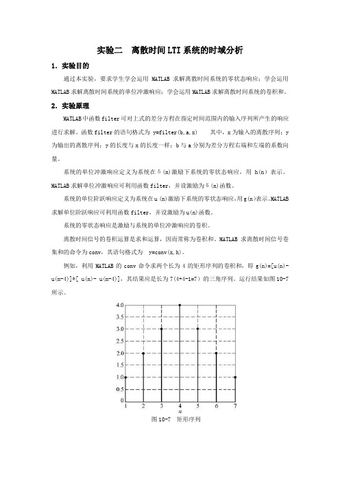
例如,利用MATLAB的conv命令求两个长为4的矩形序列的卷积和,即g(n)=[u(n)- u(n-4)]*[ u(n)- u(n-4)],其结果应是长为7(4+4-1=7)的三角序列。
运行结果如图10-7所示。
图10-7 矩形序列3.实验内容(1) 已知x(n)=u(n-“学号后两位”)-u(n-(“学号后两位”+4))、h(n)=R5(n)。
(2) 编制程序求解下列两个系统的单位冲激响应和单位阶跃响应,并绘出其图形。
(3) 已知某系统的单位冲激响应为h(n)=0.5n[u(n)-u(n-4)],试分别利用MATLAB卷积和两种方法求当激励信号为x(n)=u(n)-u(n-4)时,系统的零状态响应。
4.实验设备计算机,MATLAB软件。
数字信号处理 实验作业:离散LSI系统的时域分析

实验2 离散LSI 系统的时域分析一、.实验目的:1、加深对离散系统的差分方程、单位脉冲响应、单位阶跃响应和卷积分析方法的理解。
2、初步了解用MA TLAB 语言进行离散时间系统时域分析的基本方法。
3、掌握求解离散时间系统的单位脉冲响应、单位阶跃响应、线性卷积以及差分方程的程序的编写方法,了解常用子函数的调用格式。
二、实验原理:1、离散LSI 系统的响应与激励由离散时间系统的时域分析方法可知,一个离散LSI 系统的响应与激励可以用如下框图表示:其输入、输出关系可用以下差分方程描述:[][]NMkk k k ay n k b x n m ==-=-∑∑2、用函数impz 和dstep 求解离散系统的单位脉冲响应和单位阶跃响应。
例2-1 已知描述某因果系统的差分方程为6y(n)+2y(n-2)=x(n)+3x(n-1)+3x(n-2)+x(n-3) 满足初始条件y(-1)=0,x(-1)=0,求系统的单位脉冲响应和单位阶跃响应。
解: 将y(n)项的系数a 0进行归一化,得到y(n)+1/3y(n-2)=1/6x(n)+1/2x(n-1)+1/2x(n-2)+1/6x(n-3)分析上式可知,这是一个3阶系统,列出其b k 和a k 系数: a 0=1, a ,1=0, a ,2=1/3, a ,3=0 b 0=1/6,b ,1=1/2, b ,2=1/2, b ,3=1/6程序清单如下: a=[1,0,1/3,0]; b=[1/6,1/2,1/2,1/6]; N=32; n=0:N-1; hn=impz(b,a,n); gn=dstep(b,a,n);subplot(1,2,1);stem(n,hn,'k');课程名称 数字信号处理 实验成绩 指导教师 ***实 验 报 告院系 班级学号 姓名 日期title('系统的单位序列响应'); ylabel('h(n)');xlabel('n');axis([0,N,1.1*min(hn),1.1*max(hn)]); subplot(1,2,2);stem(n,gn,'k'); title('系统的单位阶跃响应'); ylabel('g(n)');xlabel('n');axis([0,N,1.1*min(gn),1.1*max(gn)]); 程序运行结果如图2-1所示:102030系统的单位序列响应h (n )n1020300.20.30.40.50.60.70.80.911.11.2系统的单位阶跃响应g (n )n图2-13、用函数filtic 和filter 求解离散系统的单位序列响应和单位阶跃响应。
实验二 离散时间信号与系统的时域分析

离散信号的表示离散信号的表示p124p124一个离散信号需要用两个向量来表示一个离散信号需要用两个向量来表示离散信号的幅值离散信号的幅值离散信号的位置信息离散信号的位置信息用用matlabmatlab实现离散信号的可视化实现离散信号的可视化不能利用符号运算来表示不能利用符号运算来表示绘制离散信号一般采用绘制离散信号一般采用stemstem命令
一些常用的离散信号(P134) 一些常用的离散信号(P134)
单位阶跃序列的表示:[x,n]=stepseq(n1,n2,n0)(自己 单位阶跃序列的表示:[x,n]=stepseq(n1,n2,n0)(自己 编写,参考P134,函数jyxl) 编写,参考P134,函数jyxl) function [x,n] = stepseq(n1,n2,n0) 1 n ≥ n0 u (n − n0 ) = n = [n1:n2]; 0 n < n0 x = [(n-n0) >= 0]; [(n例3:在 −5 ≤ k ≤ 5区间,画出u (k − 2)的波形
实验二 离散系统时域分析 (2学时)

数字信号处理实验指导书山东大学控制学院生物医学工程专业刘忠国2012-2-10数字信号处理实验目录实验一离散时间信号与系统分析 (3)实验二离散时间信号与系统的Z变换分析 (7)实验三IIR滤波器的设计与信号滤波 (13)实验四用窗函数法设计FIR数字滤波器 (15)实验五用FFT作谱分析 (17)实验六综合实验 (19)附录:各实验参考程序 (20)实验一 离散时间信号与系统分析一、实验目的1.掌握离散时间信号与系统的时域分析方法。
2.掌握序列傅氏变换的计算机实现方法,利用序列的傅氏变换对离散信号、系统及系统响应进行频域分析。
3.熟悉理想采样的性质,了解信号采样前后的频谱变化,加深对采样定理的理解。
二、实验原理1.离散时间系统一个离散时间系统是将输入序列变换成输出序列的一种运算。
若以][⋅T 来表示这种运算,则一个离散时间系统可由下图来表示:图 离散时间系统输出与输入之间关系用下式表示)]([)(n x T n y =离散时间系统中最重要、最常用的是线性时不变系统。
2.离散时间系统的单位脉冲响应设系统输入)()(n n x δ=,系统输出)(n y 的初始状态为零,这是系统输出用)(n h 表示,即)]([)(n T n h δ=,则称)(n h 为系统的单位脉冲响应。
可得到:)()()()()(n h n x m n h m x n y m *=-=∑∞-∞=该式说明线性时不变系统的响应等于输入序列与单位脉冲序列的卷积。
3.连续时间信号的采样采样是从连续信号到离散时间信号的过渡桥梁,对采样过程的研究不仅可以了解采样前后信号时域何频域特性发生的变化以及信号内容不丢失的条件,而且有助于加深对拉氏变换、傅氏变换、Z 变换和序列傅氏变换之间关系的理解。
对一个连续时间信号进行理想采样的过程可以表示为信号与一个周期冲激脉冲的乘积,即:)()()(ˆt t x t xT a a δ=其中,)(ˆt xa 是连续信号)(t x a 的理想采样,)(t T δ是周期冲激脉冲 ∑∞-∞=-=m T mT t t )()(δδ设模拟信号)(t x a ,冲激函数序列)(t T δ以及抽样信号)(ˆt xa 的傅立叶变换分别为)(Ωj X a 、)(Ωj M 和)(ˆΩj X a,即 )]([)(t x F j X a a =Ω )]([)(t F j M T δ=Ω)](ˆ[)(ˆt x F j X a a=Ω 根据连续时间信号与系统中的频域卷积定理,式(2.59)表示的时域相乘,变换到频域为卷积运算,即)]()([21)(ˆΩ*Ω=Ωj X j M j X aa π其中⎰∞∞-Ω-==Ωdt e t x t x F j X t j a a a )()]([)(由此可以推导出∑∞-∞=Ω-Ω=Ωk s a ajk j X T j X )(1)(ˆ 由上式可知,信号理想采样后的频谱是原来信号频谱的周期延拓,其延拓周期等于采样频率。
DSP LAB_2:离散时间系统-时域分析

姓名: 学号:班级日期:实验2离散时间系统-时域分析实验内容:2.1 SIMULATION OF DISCRETE-TIME SYSTEMSProject 2.1The Moving Average System (移动平均值系统)A copy of Program P2_1 is given below:< Insert program code here. Copy from m-file(s) and paste. > Answers:Q2.1 The output sequence generated by running the above program for M = 2 with x[n] = s1[n]+s2[n]as the input is shown below.< Insert MATLAB figure(s) here. Copy from figure window(s) and paste. >The component of the input x[n]suppressed(抑制)by the discrete-time systemsimulated by this program is -____________Q2.2Program P2_1 is modified to simulate the LTI system y[n] = 0.5(x[n]–x[n–1])and process the input x[n] = s1[n]+s2[n]resulting in the outputsequence shown below:< Insert MATLAB figure(s) here. Copy from figure window(s) and paste. >The effect of changing the LTI system on the input is - ____________Q2.3Program P2_1 is run for the following values of filter(滤波器) length M and following values of the frequencies of the sinusoidal signals s1[n]and s2[n]. The outputgenerated for these different values of M and the frequencies are shown below. Fromthese plots we make the following observations - ____________< Insert MATLAB figure(s)s here. Copy from figure window(s)s and paste. > Project 2.2 (Optional) A Simple Nonlinear Discrete-Time SystemA copy of Program P2_2 is given below:< Insert program code here. Copy from m-file(s) and paste. >Answers:Q2.4The sinusoidal signals with the following frequencies as the input signals were used to generate the output signals:____________The output signals generated for each of the above input signals are displayed below:< Insert MATLAB figure(s) here. Copy from figure window(s) and paste. > The output signals depend on the frequencies of the input signal according to thefollowing rules: ____________This observation can be explained mathematically as follows:____________Project 2.3 Linear and Nonlinear Systems(线性和非线性系统)A copy of Program P2_3 is given below:< Insert program code here. Copy from m-file(s) and paste. >Answers:Q2.5 The outputs y[n], obtained with weighted(加权的) input, and yt[n], obtained by combining the two outputs y1[n]and y2[n]with the same weights, are shownbelow along with the difference between the two signals:< Insert MATLAB figure(s) here. Copy from figure window(s) and paste. > The two sequences are -____________The system is - ____________Q2.6Program P2_3 was run for the following three different sets of values of the weighting constants(常数), a and b, and the following three different sets of input frequencies:The plots generated for each of the above three cases are shown below:< Insert MATLAB figure(s) here. Copy from figure window(s) and paste. > Based on these plots we can conclude that the system with different weights is -____________ Q2.7 Program P2_3 was modified to simulate the system:y[n] = x[n]x[n–1]The output sequences y1[n], y2[n],and y[n]of the above system generated byrunning the modified program are shown below:< Insert MATLAB figure(s) here. Copy from figure window(s) and paste. > Comparing y[n]with yt[n] we conclude that the two sequences are -____________This system is - ____________Project 2.4 Time-invariant(时不变) and Time-varying(时变) SystemsA copy of Program P2_4 is given below:< Insert program code here. Copy from m-file(s) and paste. > Answers:Q2.8The output sequences y[n]and yd[n-10] generated by running Program P2_4 are shown below -< Insert MATLAB figure(s) here. Copy from figure window(s) and paste. > These two sequences are related as follows -____________The system is -____________Q2.9The output sequences y[n]and yd[n-D] generated by running Program P2_4 for the following values of the delay variable D -are shown below - ____________< Insert MATLAB figure(s) here. Copy from figure window(s) and paste. > In each case, these two sequences are related as follows - ____________The system is -____________2.2 LINEAR TIME-INVARIANT DISCRETE-TIME SYSTEMSProject 2.5 Computation of Impulse Responses(冲击响应) of LTI SystemsA copy of Program P2_5 is shown below:< Insert program code here. Copy from m-file(s) and paste. > Answers:Q2.10 The first 41 samples of the impulse response of the discrete-time system of Project 2.3 generated by running Program P2_5 is given below:< Insert MATLAB figure(s) here. Copy from figure window(s) and paste. > Q2.11The required modifications to Program P2_5 to generate the impulse response of the following causal LTI system:y[n] + 0.71y[n-1] – 0.46y[n-2] – 0.62y[n-3]= 0.9x[n] – 0.45x[n-1] + 0.35x[n-2] + 0.002x[n-3]are given below:< Insert program code here. Copy from m-file(s) and paste. >The first 45 samples of the impulse response of this discrete-time systemgenerated by running the modified is given below:< Insert MATLAB figure(s) here. Copy from figure window(s) and paste. >Q2.12The MATLAB program to generate and plot the step response(阶跃响应) of a causal LTI system(因果线性时不变系统) is indicated below:< Insert program code here. Copy from m-file(s) and paste. >The first 40 samples of the step response of the LTI system of Project 2.3 are shown below:< Insert MATLAB figure(s) here. Copy from figure window(s) and paste. >Project 2.6 Convolution(卷积)A copy of Program P2_6 is reproduced below:< Insert program code here. Copy from m-file(s) and paste. >Answers:Q2.13 The sequences y[n] and y1[n] generated by running Program P2_6 are shown below: < Insert MATLAB figure(s) here. Copy from figure window(s) and paste. > The difference between y[n]and y1[n]is - ____________The reason for using x1[n] as the input, obtained by zero-padding(填零)x[n],for generating y1[n]is - ____________Q2.14The modified Program P2_6 to develop the convolution of a length-15 sequence h[n] with a length-10 sequence x[n]is indicated below:< Insert program code here. Copy from m-file(s) and paste. >The sequences y[n] and y1[n] generated by running modified Program P2_6 areshown below:< Insert MATLAB figure(s) here. Copy from figure window(s) and paste. > The difference between y[n] and y1[n] is - ____________Project 2.7 Stability of LTI Systems(线性时不变系统稳定性)A copy of Program P2_7 is given below:< Insert program code here. Copy from m-file(s) and paste. >Answers:Q2.15The purpose of the for command is- ____________The purpose of the end command is -____________Q2.16 The purpose of the break command is-____________Q2.17The discrete-time system of Program P2_7 is -____________The impulse response generated by running Program P2_7 is shown below:< Insert MATLAB figure(s) here. Copy from figure window(s) and paste. > The value of |h(K)| here is - ____________From this value and the shape of the impulse response we can conclude that thesystem is - ____________By running Program P2_7 with a larger value of N the new value of |h(K)|is - ____________From this value we can conclude that the system is - ____________Project 2.8 Illustration of the Filtering Concept(滤波概念的图示)A copy of Program P2_8 is given below:< Insert program code here. Copy from m-file(s) and paste. >Answers:Q2.18The output sequences generated by this program are shown below:< Insert MATLAB figure(s) here. Copy from figure window(s) and paste. >The filter with better characteristics for the suppression(抑制) of the high frequencycomponent(高频成分) of the input signal x[n]is - ____________。
- 1、下载文档前请自行甄别文档内容的完整性,平台不提供额外的编辑、内容补充、找答案等附加服务。
- 2、"仅部分预览"的文档,不可在线预览部分如存在完整性等问题,可反馈申请退款(可完整预览的文档不适用该条件!)。
- 3、如文档侵犯您的权益,请联系客服反馈,我们会尽快为您处理(人工客服工作时间:9:00-18:30)。
实验二:离散LSI 系统的时域分析
一、实验目的:
1加深对离散系统的差分方程、单位脉冲响应、单位阶跃响应的理解。
2.初步了解用MATLAB 语言进行离散时间系统时域分析的基本方法。
. 二、实验内容:
1、已知描述某离散LSI 系统的差分方程为2()3(1)(2)(1)y n y n y n x n --+-=-,分别用impz 和dstep 函数、filtic 和filter 函数两种方法求解系统的单位序列响应和单位阶跃响应。
用impz 和dstep 函数 程序如下:
a=[1,-3/2,1/2]; b=[0,1/2,0]; N=32; n=0:N-1;
hn=impz(b,a,n); gn=dstep(b,a,n);
subplot(1,2,1);stem(n,hn,'k'); title('系统的单位序列响应'); ylabel('h(n)');xlabel('n');
axis([0,N,1.1*min(hn),1.1*max(hn)]); subplot(1,2,2);stem(n,gn,'k'); title('系统的单位阶跃响应'); ylabel('g(n)');xlabel('n');
axis([0,N,1.1*min(gn),1.1*max(gn)
系统的单位序列响应h (n )
n
系统的单位阶跃响应
g (n )
n
x01=0;y01=0; a=[1,-3/2,1/2]; b=[0,1/2,0]; N=32;n=0:N-1;
xi=filtic(b,a,0); x1=[n==0];
hn=filter(b,a,x1,xi); x2=[n>=0];
gn=filter(b,a,x2,xi);
subplot(1,2,1);stem(n,hn,'k'); title('系统的单位序列响应'); ylabel('h(n)');xlabel('n');
axis([0,N,1.1*min(hn),1.1*max(hn)]); subplot(1,2,2);stem(n,gn,'k'); title('系统的单位阶跃响应'); ylabel('g(n)');xlabel('n');
axis([0,N,1.1*min(gn),1.1*max(gn)]);
系统的单位序列响应h (n )
n
系统的单位阶跃响应
g (n )
n
2、编写程序描绘下列序列的卷积波形: n1=0:10;
N1=length(n1); f1=[n1>=2];
subplot(2,2,1);stem(n1,f1,'filled'); title('f1(n)'); n2=0:10;
N2=length(n2); f2=ones(1,N2);
subplot(2,2,2);stem(n2,f2,'filled'); title('f2(n)'); y=conv(f1,f2);
subplot(2,1,2);stem(y,'filled');
f1(n)
510
f2(n)
0510152025
5
10
15
N=32;nt=1;n=-3:4*pi; f1=sin(n/2)
subplot(2,2,1);stem(n,f1,'filled'); title('f1(n)'); n2=-3:4*pi; f2=0.5.^n2
subplot(2,2,2);stem(n2,f2,'filled'); title('f2(n)'); y=conv(f1,f2);
subplot(2,1,2);stem(y,'filled');
-1-0.500.51f1(n)
02468f2(n)
05101520253035
-20
-10010
20
3、已知某离散LSI 系统的单位序列响应为
()3(3)0.5(4)0.2(5)0.7(6)0.8(7)h n n n n n n δδδδδ=-+-+-+---
求输入为0.5()()n
x n e u n -=时的系统响应。
程序如下: n1=3:7;
h(n1)=[3,0.5,0.2,0.1,-0.8];
subplot(2,2,1);stem(n1,h(n1),'filled'); title('h(n1)'); n=10; n2=1:n;
g(n2)=exp(-0.5*n2);
subplot(2,2,2);stem(n2,g(n2),'filled'); title('g(n2)'); y=conv(h(n1),g(n2));
subplot(2,1,2);stem(y,'filled'); title('y')
图形为:
4
已知描述某离散LSI 系统的差分方程为()0.7(1)2()(2)y n y n x n x n =-+--,求输入为
()(3)x n u n =-时的系统响应。
程序如下:
a=[1,-0.7,0]; b=[2,0,-1]; N=25;n=0:N-1; xi=filtic(b,a,0); x=[n>=3];
gn=filter(b,a,x,xi); stem(n,gn,'filled'); title('ϵͳÏìÓ¦');
ylabel('g(n)');xlabel('n');
axis([0,N,1.1*min(gn),1.1*max(gn)]);
图形为:
(1)通过本次试验加深了对离散系统的差分方程、单位脉冲响应、单位阶跃响应和卷积分析方法的理解。
用MATLAB编程能很简单的实现系统的卷积和响应。
MATLAB中丰富的函数库为我们编程提供很大的便利。
(2)本实验学习的新函数conv是难点也是重点,它能实现对系统的卷积积分,卷积函数conv默认两个序列的序号均从n=0开始,卷积结果y对应的序列的序号也是从N=0开始的。
要注意conv( )函数和各序列长度的计算,写错将会影响实验的结果。