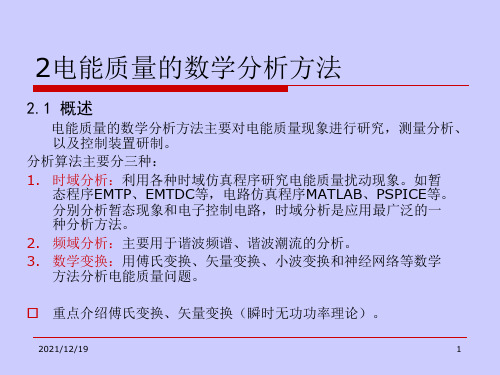
2 瞬时功率理论
旋转p-q-r坐标系下的瞬时功率理论
旋转p-q-r坐标系下的瞬时功率理论摘要该论文在三相四线制系统中定义了一个旋转的p-q-r坐标系,这里,p为瞬时有功功率,为瞬时无功功率。
这三个分量是线性独立的,所以可以通过单独控制两个电流分量的空间矢量来补偿这两个瞬时无功功率。
该论文按照这个理论,通过补偿瞬时无功功率来消除三相四线制系统的中线上的电流,而无需储存能量,仿真的结果很好地证明了这个理论。
1引言韩国和美国等其他国家,不低于70%的电能消费用于电机,主要是感性电机。
如果假设电机负载的功率因数是0.8,那么发电厂最少得发出17%的无功功率,这就需要更多的发电机,并且增加了传输/分布损耗。
换句话说,如果完全补偿用户侧的无功功率,那么发电设备和分布损耗将最少减少17%。
除此之外,当三相四线制系统接不平衡或非线性负载时,流过中线上的电流将很大。
在单相二极管整流的情况下,流过中线的电流为相电流的1.73倍。
由于传统的三相四线制系统的中线不能解决上述问题,并且存在大量的电力电子设备,会在用户侧产生大量问题。
三相系统中,瞬时无功电流产生不产生瞬时有功功率。
所以由补偿无功功率来控制无功电流不需要储备能量的设备,如三相系统中功率补偿器的直流侧电容。
这样能够降低成本,提高功率补偿的可靠性。
三相系统中,瞬时有功和无功功率分别定义为电压矢量和电流矢量的内积和矢量积。
瞬时有功功率是线性独立的,但是瞬时无功功率的三个分量却不是彼此独立的。
也就是说,可以单独的补偿瞬时有功功率,却不能单独各自补偿瞬时无功功率的三个分量。
因此,瞬时无功功率的补偿电流的自由度是1。
系统的零序电压和零序电流既影响瞬时有功功率,又影响瞬时无功功率。
当电源电压中有零序分量时,即使把瞬时无功功率补偿到零,中线电流也不会完全消除。
[8]中采用了特殊的无功功率补偿算法,来消除三相四线制系统中的中线电流,但这种算法仍然受电流只有一个可控量的限制。
该论文提出了一个所谓的p-q-r坐标系,它能随着三相四线制系统的电压空间矢量旋转。
2单相无功瞬时值定义的应用-电测与仪表

基于瞬时无功理论的单相无功功率相关定义高宇澄,赵伟,黄松岭(清华大学电机系电力系统国家重点实验室,北京100084)摘要:1983年Akagi提出的瞬时无功理论具有计算量小、瞬时性好等优点,但不能直接应用于单相电路的分析。
一些学者借鉴瞬时无功理论,通过α−β变换将电压、电流信号映射至二维空间的思路,提出了多种定义单相电路瞬时无功功率量值的理论。
本文试对这一类单相瞬时无功功率定义多年来的研究成果加以综述。
具体地,将整理广义瞬时功率理论、无功电流理论、瞬时无功密度理论这三类有关单相电路瞬时无功功率的定义,并介绍瞬时无功功率理论在测量基波无功、谐波电流以及控制锁相环电路方面的应用。
最后,试分析现有单相瞬时无功功率理论的局限性。
关键词:无功功率;瞬时无功功率理论;瞬时功率;功率测量;单相电路中图分类号:TM930 文献标识码:A 文章编号:1001-1390(2016)20-0000-00 Reactive power definitions in single-phase circuits based on instantaneousreactive power theoryGao Yucheng, Zhao Wei, Huang Songling(State Key Laboratory of Power System, Tsinghua University, Beijing 100084, China)Abstract:Presented by Akagi and coauthors in 1983, instantaneous reactive power theory (IRP theory) features low computational complexity and good instantaneity, but it is not directly applicable to single-phase circuits. Scholars have been developed new approaches to define reactive power in single-phase circuits by utilizing the idea of IRP theory, thus mapping the voltage and current signals to a two-dimensional space with α−βtransformation. This paper presents an overview of the reactive power definitions in single-phase circuits that are particularly based on IRP theory. Specifically, 3 types of definitions are summarized as follows: generalized instantaneous reactive power theory, reactive current theory, and instantaneous reactive power density theory, as well as introduces the application of instantaneous reactive power theory on measuring fundamental reactive power, harmonic current, and controlling the phase-locked loop circuit. Furthermore, the limitation of existing single phase instantaneous reactive power theory is analyzed.Keywords:reactive power, instantaneous reactive power theory, instantaneous power, power measurement, single-phase circuit0引言无功功率是电路理论中的重要物理量,用来表征电路网络之间反复交换的功率的最大幅度。
瞬时功率理论 ppt

赤木泰文介绍:赤木泰文(HirofumiAkagi),日本东京技术学院 (TokyoInstituteofTechnology)电气工程学教授,讲授电力电子 学。1996年当选为IEEE会士(1EEEFellow).1998~1999年被 选为IEEE工业应用学会和电力电子学会的杰出演讲者,2001年 获得国际电力电子学领域的最高奖——IEEEWilliamE.Neweli 奖.2004年获得IEEE工业应用学会杰出成就奖。
pt et i t e(t )T i (t ) cos
T
定义有功分量 i p 为电流向量 i (t ) 在电压向量 e(t )上的正 交投影,则 i p i cos .
e(t )T i (t ) e(t ) p (t ) ip e(t ) 2 e(t ) e(t ) e(t )
Akagi瞬时无功功率的不足之处: (1) 只适用于无零序电流和电压分量的三相系统; (2)只能用于三相系统,不能推导单相、多相的 情况
2.3.3 基于电流分解的瞬时无功功率
不直接对功率进行分解,而是将电流分解为平行 于电压的有功分量和垂直于电压的无功分量。
将瞬时功率定义为电压向量和电流向量的内积:
其中
1 1 1 2 2 2 C32 3 3 3 0 2 2
定义瞬时有功功率为: p(t ) e i e i eaia ebib ecic 定义瞬时无功功率为: q(t ) e i e i
α、β平面上的瞬时有功电流 i p 和瞬时无功电流 iq 分 别为瞬时空间矢量i在瞬时空间矢量电压e及其法线上 的投影 i i cos, i i sin
现代电力电子技术
——2.3 瞬时功率理论
瞬时功率理论及其应用研究
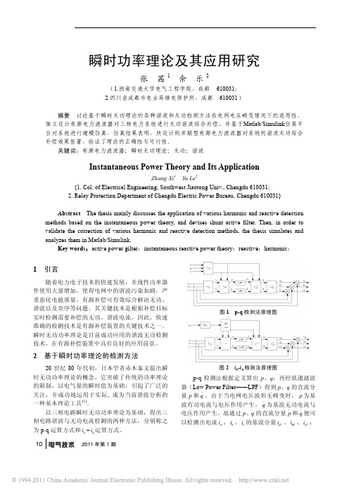
2011年第1期10瞬时功率理论及其应用研究张 茜1 余 乐2(1.西南交通大学电气工程学院,成都 610031; 2.四川省成都市电业局继电保护所,成都 610031)摘要 讨论基于瞬时无功理论的各种谐波和无功检测方法在电网电压畸变情况下的适用性,独立设计有源电力滤波器对三相电力系统进行无功谐波综合补偿,并基于Matlab/Simulink 仿真平台对系统进行建模仿真,仿真结果表明,所设计的并联型有源电力滤波器对系统的谐波无功综合补偿效果显著,验证了理论的正确性与可行性。
关键词:有源电力滤波器;瞬时无功理论;无功;谐波Instantaneous Power Theory and Its ApplicationZhang Xi 1 Yu Le 2(1. Col. of Electrical Engineering, Southwest Jiaotong Univ., Chengdu 610031; 2. Relay Protection Department of Chengdu Electric Power Bureau, Chengdu 610031)Abstract The thesis mainly discusses the application of various harmonic and reactive detection methods based on the instantaneous power theory, and devises shunt active filter. Then, in order to validate the correction of various harmonic and reactive detection methods, the thesis simulates and analyzes them in Matlab/Simulink.Key words :active power gilter ;instantaneous reactive power theory ;reactive ;harmonic ;1 引言随着电力电子技术的快速发展,非线性功率器件使用大量增加,使得电网中的谐波污染加剧,严重恶化电能质量。
2电能质量分析与控制
2021/12/19
18
2电能质量的数学分析方法
2、快速傅里叶变换的应用
FFT在谐波分析仪、电能质量分析仪(离线)、电能质量在线监 测装置中的应用: 同时采集u、I信号,通过FFT分析给出各次谐波幅值、相角、功率 等。
75点:-2.2199E-13 -1.0076E-12i 76点:3.4315E-12 + 192i 77点:-3.0263E-14 +7.5609E-13i
很明显,1点、51点、76点的值都比较大,
附近的点值都很小,可以认为是0,即在那些频率点上的信号幅度为0。
2021/12/19
14
2电能质量的数学分析方法
如果要提高频率分辨率,则必须增加采样点数,也即采样时间。频率分 辨率和采样时间是倒数关系。
2021/12/19
12
2电能质量的数学分析方法
信号的时长的截取
截取信号的时长(N数值)决定了所需分开的两个频率之间的最小的频 率间隔。
如:相邻的最小频率间隔是10.2-10=0.2Hz,也就是说你需要把10 和10.2Hz这两个成分分开即可(如果分辨率太高则数据量太长, 浪费计算时间,如果分辨率太低,则无法把这两个频率分开), 所以可以选择截取的最小时长为t=1/(10.2-10)=5秒。
X (k ) F[x(n)] x(n)e N
n0
利用欧拉公式可以证明:
(k = 0,1, ,N-1)
可见:利用matlab中的函数FFT计算出X(K)乘以2/N,再求模即可 得到上述基于连续信号傅立叶级数的各次谐波幅值计算公式,即 得到各次谐波的真正幅值。
瞬时功率.PPT

瞬时功率理论谐波检测方法的仿真模型研究
在
平面上 , 矢量 , 和 , 分别合成 ( 旋
v = v  ̄ + v o / _ q o ( 3 )
转) 电压矢 量 和电流 矢量 i 。
电 力 系 统 中 的 应 用 日益 增 多 , 导 致 大 量 谐 波 注 入 电
网, 并 引起 电网闪 变 、 频率 变 化 、 三 相不 平 衡 等 问题 ,
进 而 对 电能 质 量 、输 电效率 和设 备安 全 运行 造 成 影 响 。 目前 ,谐 波 抑 制 的 主要 趋势 是 利用 有 源 滤波 器 ( A P F ) 进 行 补偿 , 但其 补偿 特性 取 决 于负 荷 电流 中提
收 稿 日期 : 2 0 1 3 — 0 2 — 2 8
逆。
作者简 介 : 刘长亮( 1 9 8 7 一) , 男, 硕士, 从 事 有 源 电 力 滤 波 器谐
波检 测 方 法 的 研 究 。
该方 法 由定 义计 算 的 P, q经低 通 滤 波 器 L P F滤
2 0 1 3年 第 5期
摘要 : 介 绍 瞬 时 功 率 理 论 以及 基 于 其 理 论 的 两 种谐 波 检 测 方 法 。利 用 MA T L A B仿 真软 件 中 的 S i m P o w e r 工具 箱 对 谐 波 电流 检 测 方 法进行建模和仿真 . 详 细 介 绍 仿 真模 型 的建 立 方 法及 各 个 模 块 的仿 真 模 型 , 通 过 仿 真 研 究 验证 两 种谐 波 检测 方法 的 正 确性 和措 施 的有 效 性 。
瞬时功率理论及其在电力调节中的应用_pref
.
xiv
PREFACE
Chapter 4 is exclusively dedicated to shunt active filters with different filter structures, showing clearly whether energy storage elements such as capacitors and inductors are necessary or not, and how much they are theoretically dispensable to the active filters. This consideration of the energy storage elements is one of the strongest points in the instantaneous power theory. Chapter 5 addresses series active filters, including hybrid configurations of active and passive filters. The hybrid configurations may provide an economical solution to harmonic filtering, particularly in medium-voltage, adjustable-speed motor drives. Chapter 6 presents combined series and shunt power conditioners, including the unified power quality conditioner (UPQC), and the unified power flow controller (UPFC) that is a FACTS (flexible ac transmission system) device. Finally, it leads to the universal active power line conditioner (UPLC) that integrates the UPQC with the UPFC in terms of functionality. Pioneering applications of the p-q theory to power conditioning are illustrated throughout the book, which helps the reader to understand the substantial nature of the instantaneous power theory, along with distinct differences from conventional theories. The authors would like to acknowledge the encouragement and support received from many colleagues in various forms. The first author greatly appreciates his former colleagues, Prof. A. Nabae, the late Prof. I. Takahashi, and Mr. Y. Kanazawa at the Nagaoka University of Technology, where the p-q theory was born in 1982 and research on its applications to pure and hybrid active filters was initiated to spur many scientists and engineers to do further research on theory and practice. The long distance between the homelands of the authors was not a serious problem because research-supporting agencies like CNPq (Conselho Nacional de Desenvolvimento Científico e Tecnoló gico) and JSPS (the Japan Society for the Promotion of Science) gave financial support for the authors to travel to Brazil or to Japan when a conference was held in one of these countries. Thus, the authors were able to meet and discuss face to face the details of the book, which would not be easily done over the Internet. The support received from the Fundação de Amparo à Pesquisa do Estado do Rio de Janeiro (FAPERJ) is also acknowledged. Finally, our special thanks go to the following former graduate students and visiting scientists who worked with the authors: S. Ogasawara, K. Fujita, T. Tanaka, S. Atoh, F. Z. Peng, Y. Tsukamoto, H. Fujita, S. Ikeda, T. Yamasaki, H. Kim, K. Wada, P. Jintakosonwit, S. Srianthumrong, Y. Tamai, R. Inzunza, and G. Casaravilla, who are now working in industry or academia. They patiently helped to develop many good ideas, to design and build experimental systems, and to obtain experimental results. Without their enthusiastic support, the authors could not have published this book. H. AKAGI, E. H. WATANABE, AND M. AREDES Tokyo/Rio de Janeiro, August, 2006
关于瞬时无功功率理论的探讨
关于瞬时无功功率理论的探讨山 霞(武汉大学电气工程学院,武汉430072)摘 要:通过瞬时无功功率P-Q理论(IR P)及电流物理分量理论(CP C)在电网电压、电流为正弦的三相三线制不对称电路中的应用的对比,表明瞬时无功功率理论的分析结果与电路中的某些功率现象不一致:即无功功率Q 为零时,瞬时无功电流可能不为零;有功功率P为零时,瞬时有功电流不为零;电源电压为正弦,负荷为非谐波源时,瞬时有功电流和瞬时无功电流中都包含三次谐波分量。
瞬时有功功率p、瞬时无功功率q与有功功率P、无功功率Q及不平衡功率D之间的关系说明p、q分别与多个功率现象相关,仅用P、Q的瞬时值不能无延时的辨识三相负荷不对称系统的功率特性。
这一结论对有源电力滤波器的控制算法具有重要意义。
关键词:瞬时无功功率理论;电流物理分量理论;有源滤波器;不对称系统;控制算法中图分类号:T M71文献标识码:A文章编号:1003 6520(2006)05 0100 03Discussion on Instantaneous Reactive Power P Q TheorySH AN Xia(School of Electrical Eng ineer ing,Wuhan U niv ersity,Wuhan430072,China)Abstract:T he compariso n of the instant aneous reactive power P Q theo ry(IR P)wit h the t heo ry o f the cur rent's physical components(CP C)presented in this pa per reveals t he results of t he IR P P Q theor y are inconsistent w ith po wer phenomena in three phase,three w ir e cir cuit s w ith sinusoidal vo ltag es and curr ents.N amely,according to the IR P P Q T heor y the instantaneous reactive cur rent can occur ev en if a load has zero reactive power Q.Similarly, the instantaneo us activ e cur rent can o ccur ev en if a load has zero act ive pow er P.M or eover,t hese tw o cur rents in circuits w ith a sinusoidal supply v oltage can be nonsinusoidal even if there is no so ur ce of cur rent distor tio n in the load.T he relat ionship betw een the instantaneous pow ers(p,q)and the activ e,reactiv e and unba lanced po wer(P, Q,D)sho ws the p and q po wer s ar e associated w ith multiple phenomenon,and the IR P P Q T heor y can no t identify po wer propert ies o f thr ee phase unbalanced loads w ith a pair of values of p and q po wer s instantaneo usly.T his con clusio n may have an impo rtant va lue for co ntr ol alg or ithms of activ e pow er f ilter s.Key words:instantaneous reactive pow er theor y;theor y of curr ent s physical components;act ive po wer f ilter s;un balanced sy stems;co nt rol alg or ithms0 引 言为解决谐波、无功功率的瞬时检测和不用储能元件实现二者补偿的问题,Akag i提出的瞬时无功功率P Q理论(IRP)[1 4],是脉冲宽度调制(PWM)技术及有源滤波器的数学基础,极大推动谐波和无功补偿装置的研究开发,是分析非正弦三相电路功率特性的理论工具[5 12]。
p-q理论
p-q 理论一、p-q 理论基础p-q 理论的基础是一系列在时域中定义的瞬时功率,该理论对电压和电流的波形没有任何限制,适用于有中性线或无中性线的任何三相系统。
因此,这种理论不但适合用于稳态,而且也适用于暂态。
P-q 理论首先将电压和电流从abc 坐标系变换到o αβ坐标系,然后在o αβ坐标系中定义瞬时功率。
因此,p-q 理论总是将三相系统作为一个单元来考虑,而不是将三相系统作为三个单相系统的叠加来处理。
1、clarke 变换o αβ变换即clarke 变换,将abc 坐标系中的三相瞬时电压a v 、b v 和c v 影射到o αβ坐标系中的瞬时电压v α、v β和o v 。
对于任何三相电压,clarke 变换和它的反变换如下:11122o a b c v v v v v v αβ⎤⎥⎡⎤⎥⎡⎤⎢⎥⎥⎢⎥=--⎢⎥⎥⎢⎥⎢⎥⎢⎥⎣⎦⎣⎦⎢⎢⎣⎦其反变换为101212a obc v v v v v v αβ⎤⎥⎥⎡⎤⎡⎤⎥⎢⎥⎢⎥=-⎥⎢⎥⎢⎥⎢⎥⎢⎥⎣⎦⎣⎦⎢-⎦类似的,对于任何三相电流a i 、b i 和c i ,可以用下式将其变换到o αβ坐标系。
11122o abci ii ii iαβ⎤⎥⎡⎤⎥⎡⎤⎢⎥⎥⎢⎥=--⎢⎥⎥⎢⎥⎢⎥⎢⎥⎣⎦⎣⎦⎢⎢⎣⎦电流的反变换为101212a obci ii ii iαβ⎤⎥⎥⎡⎤⎡⎤⎥⎢⎥⎢⎥=-⎥⎢⎥⎢⎥⎢⎥⎢⎥⎣⎦⎣⎦⎢-⎦2、p-q理论定义的瞬时功率在三相系统中,三个瞬时功率,即瞬时零序功率o p、瞬时实功率p和瞬时虚功率q是基于oαβ坐标系下的瞬时相电压和瞬时线电流来定义:二、三相三线制系统中的p-q理论p-q理论的一个重要应用是用来补偿不合理的电流。
在三相三线制系统中不存在零序分量,故0ov=且0oi=。
设av、bv和cv,ai、bi和ci为采样所得三相的电压和电流,则clark变换为1112222abcvvvvvαβ⎤⎡⎤--⎥⎡⎤⎢⎥=⎢⎥⎢⎥⎣⎦⎢⎥-⎣⎦⎣⎦1112222abciiiiiαβ⎡⎤⎡⎤--⎢⎥⎡⎤⎢⎥⎢=⎢⎥⎢⎥⎢⎣⎦⎢⎥-⎣⎦⎢⎣⎦通过p-q理论中瞬时功率的定义得到系统瞬时有功功率和瞬时无功功率00o o op v ip v v iq v v iαβαβαβ⎡⎤⎡⎤⎡⎤⎢⎥⎢⎥⎢⎥=⎢⎥⎢⎥⎢⎥⎢⎥⎢⎥⎢⎥-⎣⎦⎣⎦⎣⎦v v i p v v i q αβαβαβ⎡⎤⎡⎤⎡⎤=⎢⎥⎢⎥⎢⎥-⎣⎦⎣⎦⎣⎦通过上式计算得到的瞬时实功率可以被分解为平均部分p 和振荡部分p ;同样,负载的虚功率q 也可以被分解为平均部分q 和振荡部分q 。
- 1、下载文档前请自行甄别文档内容的完整性,平台不提供额外的编辑、内容补充、找答案等附加服务。
- 2、"仅部分预览"的文档,不可在线预览部分如存在完整性等问题,可反馈申请退款(可完整预览的文档不适用该条件!)。
- 3、如文档侵犯您的权益,请联系客服反馈,我们会尽快为您处理(人工客服工作时间:9:00-18:30)。
−1 pq
u β iα iα i = C pq i − uα β β
1 = 2 2 − uα − u β
− uα − u β − u uα β 1 uα u β 1 = 2 u − u = 2 C pq 2 uα + u β β u α
p = ua ia + ubib + uc ic
1 q= [(ub − uc )ia + (uc − ua )ib + (ua − ub )ic 3
可见, 可见,三相电路的瞬时有功功率就是三相 电路的瞬时功率。 电路的瞬时功率。
uα uα p uα uα iαp = i p cos ϕu = i p = p = 2 p= 2 2 u u u u uα + u β
ua ub uc ia ib ic
C32
uα uβ
_ iaf _ ⊗+ ibf icf _ ⊗ ⊗+ +
iα
p
p
−1 C pq
iαf C 23
iah
C32
iβ
C pq
q
q
i βf
ibh ich
ua ub uc ia ib ic
C32
uα uβ
_ iapf ⊗+ ibpf _ icpf _ ⊗ ⊗+ +
q = u i p = u i sin ϕ = u i sin(ϕu − ϕi ) = u i (sin ϕu cos ϕi − cos ϕu sin ϕi ) = u sin ϕu i cos ϕi − u cos ϕu i sin ϕi = uβ iα − uα iβ
p uα = q u β
2 uα iap = p 2 2 3 uα + u β
0 uα p u2 + u2 3 α β 2 uβ p 2 2 3 uα + u β − 2
• 传统功率理论中的有功功率 、 无功功率等 传统功率理论中的有功功率、 都是在平均值基础或相量意义上定义的, 都是在平均值基础或相量意义上定义的 , 它们只适用与电压、 它们只适用与电压 、 电流为正弦波时以及 稳态的情况。 稳态的情况 。 而瞬时无功功率理论中的概 念都是在瞬时值的基础上定义的, 念都是在瞬时值的基础上定义的 , 它不仅 适用于正弦波, 适用于正弦波 , 也适用于非正弦波和任何 过渡过程的情况。 从以上定义可以看出, 过渡过程的情况 。 从以上定义可以看出 , 瞬时无功功率理论中的概念, 瞬时无功功率理论中的概念 , 在形式上和 传统理论非常相似, 传统理论非常相似 , 可看成是传统理论的 推广和延伸。 推广和延伸。
uβ p uβ uβ iβp = i p sin ϕ u = ip = = 2 p= 2 p 2 u u u u uα + u β
uβ
uβ q uβ uβ iαq = iq sin ϕ u = iq = = 2q= 2 q 2 u u u u uα + u β
− uα − uα q − uα − uα iβq = −iq cos ϕu = iq = = 2 q= 2 q 2 u u u u uα + u β
Im
0 & Iq
& Ip
ϕ
& U
& I
Re
β
uβ
u
i βp
ip
i
iβ
ϕ
ϕu
ϕi
iαp
uα
iαq
iα
α
i βq
iq
p = u i p = u i cos ϕ = u i cos(ϕu − ϕ i ) = u i (cos ϕ u cos ϕi + sin ϕu sin ϕ i ) = u cos ϕu i cos ϕ i + u sin ϕ u i sin ϕi = uα iα + u β iβ
ua
PLL
sin − cos
iα
C
ia ib ic
′ C32
ip
iq
ip
C
′ C 23
iβ
ia 2 f ib 2 f ic 2 f
iq
q = u β iα − uα iβ = 3UI [sin ωt cos(ωt − ϕ ) − cos ωt sin(ωt − ϕ )] = 3UI sin ϕ
• 由上面的分析不难看出 , 瞬时功率理论包 由上面的分析不难看出, 容了传统的功率理论, 容了传统的功率理论 , 比传统理论有更大 的适用范围。 的适用范围。
∞
− cos ωt iα i − sin ωt β
∑ I n cos[(1 m n)ωt m ϕ n )] n =n)ωt − ϕ )] n ∑ n n =1
p uα u β iα q = u − u i α β β ∞ ∞ ∞ ∑ U n I n cos(θ n − ϕ n ) + ∑ ∑ U n I m cos[(n m m)ωt + (θ n m ϕ n )] n =1 m =1( m ≠ n ) = 3 ∞n =1 ∞ ∞ ± U I sin(θ − ϕ ) + m U n I m cos[(n − m)ωt + (θ n − ϕ n )] ∑ m=1∑≠n) n n n n ∑ n =1 n =1 (m
uβ 0 −1 0 = C23C pq − uα q q
ua ub uc
ia ib ic
C32
uα uβ
iα
C32
iβ
C pq
−1 C pq
iαq
q
iβq
C 23
iaq ibq icq
i p sin ωt i = q − cos ωt
p uα q = u β
u β iα iα i = C pq i − uα β β
p = uα iα + u β iβ = 3UI [sin ωt sin(ωt − ϕ ) + cos ωt cos(ωt − ϕ )] = 3UI cos ϕ 3UI
与电网电压没有畸变时的结果相比,误差为: 与电网电压没有畸变时的结果相比,误差为:
∆iaf 1 1 pq ∆ibf = 2 C 23C pq − 2 C 23C ′ u ∆icf u uαh = C 23 { u βh p u p u
2
+ u βh − uαh
2 瞬时功率理论
• 传统电力系统控制装置的响应时间大多在 数十毫秒到秒级, 数十毫秒到秒级 , 而基于电力电子开关的 新型控制装置的响应时间则在微妙到毫秒 远远小于电力系统20ms的工频周期。 的工频周期。 级,远远小于电力系统 的工频周期
• 传统电力系统的交流电压和电流的有效值 、 传统电力系统的交流电压和电流的有效值、 有功功率、 有功功率 、 无功功率的概念都是建立在工 频周期的基础上。 频周期的基础上 。 而对于时间常数小于工 频周期的FACTS装置 , 采用传统的功率定 装置, 频周期的 装置 义 , 无法准确描述装置在一个时间常数的 时间内有功功率和无功功率的变化。 时间内有功功率和无功功率的变化 。 为了 准确描述小于工频周期的FACTS装置的状 准确描述小于工频周期的 装置的状 需要能描述功率、 态 , 需要能描述功率 、 电压瞬时变化的瞬 时有功功率、 瞬时无功功率、 瞬时电压、 时有功功率 、 瞬时无功功率 、 瞬时电压 、 电流等概念。 电流等概念。
ua = 2U sin ωt ia = 2 I sin(ωt − ϕ ) 2π 2π ub = 2U sin(ωt − ), ib = 2 I sin(ωt − ϕ − ) 3 3 2π 2π uc = 2U sin(ωt + 3 ) ic = 2 I sin(ωt − ϕ + 3 )
uβ
从定义3很容易得到以下性质: 从定义 很容易得到以下性质: 很容易得到以下性质
i +i = i
(1)
2 αp 2 αq 2 βp 2 βq
2 p
i +i = i
2 q
iαp + iαq = iα
(2)
iβ p + iβ q = iβ
1 iap 1 iαp 2 − ibp = C23 = 3 2 iβp icp 1 − 2
iα
C32
iβ
C pq
p q
p
−1 C pq
iαf
C 23
iβf
iad ibd icd
uβ iaq u2 + u2 iαq β ibq = C23 = C23 α − uα iβq icq u2 + u2 β α
q 1 uα = C23 2 2 uα + u β u β q
2
I1 sin(−ϕ1 ) q p I1 cos ϕ1 q ) + u βf ( 2 − ) 2 uαf ( 2 − U U1 u u u 1 } + q I1 sin(−ϕ1 ) p I1 cos ϕ1 q ) + uαf ( 2 − ) 2 u βf ( 2 − U U1 u u u 1