Plotting with Two Y-Axes __ Basic Plotting Commands (Graphics)

合集下载

实验二MATLAB基础知识(二)

Experiment 1.Fundamental Knowledge of Matlab (II> 【Experimental Purposes】1、熟悉并掌握MATLAB的工作环境。

2、运行简单命令，实现数组及矩阵的输入输出，了解在MATLAB下如何绘图。

【Experimental Principle】1. VectorsLet's start off by creating something simple, like a vector. Enter each element of the vector (separated by a space> between brackets, and set it equal to a variable. For example, to create the vector a, enter into the MATLAB command window (you can "copy" and "paste" from your browser into MATLAB to make it easy>: b5E2RGbCAPa = [1 2 3 4 5 6 9 8 7]MATLAB should return:a =1 2 3 4 5 6 9 8 7To generate a series that does not use the default of incrementing by 1, specify an additional value with the colon operator (first:step:last>. In between the starting and ending value is a step value that tells MATLAB how much to increment (or decrement, if step is negative> between each number it generates. To generate a vector with elementsbetween 0 and 20, incrementing by 2(this method isfrequently used to create a time vector>, usep1EanqFDPw t = 0:2:20t =0 2 4 6 8 10 12 14 16 18 20Manipulating vectors is almost as easy as creating them. First, suppose you would like to add 2 to each of the elements in vector 'a'. The equation for that looks like: DXDiTa9E3db = a + 2b =3 4 5 6 7 8 11 10 9Now suppose, you would like to add two vectors together. If the two vectors are the same length, it is easy. Simply add the two as shown below: RTCrpUDGiTc = a + bc =4 6 8 10 12 14 20 18 16Subtraction of vectors of the same length works exactly the same way.5PCzVD7HxAMATLAB sometimes stores such a list in a matrix withjust one row, and other times in a matrix with just one column. In the first instance, such a 1-row matrix is called a row-vector。

ANSYS常见警告信息相关解释

ANSYS常见警告信息相关解释NO.0001、ESYS is not valid for line element.原因：是因为我使用LATT的时候，把“--”的那个不小心填成了“1”。

经过ANSYS的命令手册里说那是没有用的项目，但是根据我的理解，这些所谓的没有用的项目实际上都是ANSYS在为后续的版本留接口。

对于LATT，实际上那个项目可能就是单元坐标系的设置。

当我发现原因后，把1改成0——即使用全局直角坐标系，就没有WARNING了。

当然，直接空白也没有问题。

NO.0002、使用*TREAD的时候，有的时候明明看文件好好的，可是却出现*TREAD end-of-file in data read.后来仔细检查，发现我TXT的数据文件里，分隔是采用TAB键分隔的。

但是在最后一列后面，如果把鼠标点上去，发现数据后面还有一个空格键。

于是，我把每个列最后多的空格键删除，，然后发现上面的信息就没有了。

NO.0003、Coefficient ratio exceeds1.0e8-Check results.这个大概是跟收敛有关，但是我找不到具体的原因。

我建立的一个桥梁分析模型，尽管我分析的结果完全符合我的力学概念判断，规律完全符合基本规律，数据也基本符合实际观测，但是却还是不断出现这个警告信息。

有人知道这个信息是什么意思，怎么调试能消除吗？NO.0004、*TREAD end-of-file in data readtxt中的表格数据不完整！NO.0005、No*CREATE for*END.The*END command is ignored忘了写*END了吧。

NO.0006、Keypoint1is referenced by only one line.Improperly connected line set for AL command两条线不共点,尝试nummrg命令NO.0007、L1is not a recognized PREP7command,abbreviation,or macro.This command will be ignored还没有进入prep7，先：/prep7NO.0008、Keypoint2belongs to line4and cannot be moved同一位置点2已经存在了，尝试对同位置的生成新点换个编号，比如1002NO.0009、Shape testing revealed that32of the640new or modified elementsviolate shape warning limits.To review test results,please see theoutput file or issue the CHECK command.单元形状奇异，在我的模型中6面体单元的三个边长差距较大，可忽略该错误。

第五讲奥肯定律与菲利普斯曲线

ut − ut −1 = − 0.4( g yt − 3%)
Changes in the Unemployment Rate Versus Output Growth in the United States, 1970-2000 1970-
ut − ut −1 = − 0.4( g yt − 3%)
§2. The Phillips Curve: From Curve: Unemployment to Inflation
In 1958, A.W.Phillips drew a diagram π plotting the rate of inflation against the PC rate of unemployment in the United Kingdom for each year from 1861 to 1957. He found a clear evidence of a negative relation between inflation and unemployment: When unemployment was low, inflation was high, and when unemployment was high, inflation was low, often even negative. 0 u Two years later, Paul Samuelson and Robert Solow replicated Phillips’ exercise for the United States, there • Samuelson and Solow appeared to be a negative relation baptized this relation the between inflation and unemployment in Phillips Curve. the United States also.

matlabref

[ 1 2; 3 4]
zeros(n) ones(n) zeros(m,n) ones(m,n) ones(A)
creates a m-row, n-column matrix of zeros.
1 2 Create the matrix . 3 4 creates an nxn matrix whose elements are zero.
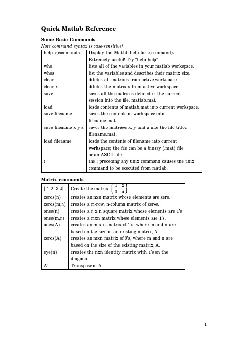
Quick Matlab Reference
Some Basic Commands Note command syntax is case-sensitive! help <command> Display the Matlab help for <command>. Extremely useful! Try “help help”. who whos clear clear x save load save ﬁlename save ﬁlename x y z load ﬁlename lists all of the variables in your matlab workspace. list the variables and describes their matrix size. deletes all matrices from active workspace. deletes the matrix x from active workspace. saves all the matrices deﬁned in the current session into the ﬁle, matlab.mat. loads contents of matlab.mat into current workspace. saves the contents of workspace into ﬁlename.mat saves the matrices x, y and z into the ﬁle titled ﬁlename.mat. loads the contents of ﬁlename into current workspace; the ﬁle can be a binary (.mat) ﬁle or an ASCII ﬁle. ! the ! preceding any unix command causes the unix command to be executed from matlab. Matrix commands

EBSD数据分析

Access to routines that cleanup the dataset
Use this to export text .ang files
Access to menu for: - Maps - Texture calculation - Texture plots
Export grain ID data associated with each point
- If both conditions are met, the -pCorienat’tseo“rcielenatnaetiodnuips” cdhaotasesenttaos abeneawnediagthabsoert’s at random - Repeat low cleanup levels -(Wn=ri3temthaex)“culnetailnneod mupo”redaptoaisnetst dcihreacntglyetfoorfilbeest results
Selection formula is explicitly written here
Data Cleanup
GGNNrreaeaiigingnhhDbCbioIlaorStrCitoaPOInnCh:rdiaoearsrnrdeeti.lzaCCatiotooiornrnree:lalattioionn
Note: Points that are excluded are given a grain ID of 0 (zero) in exported files
Grain Definitions
Examples of definitions
3 degrees
15 degrees
Note that each color represents 1 grain

eetop[1].cn_Inspect

InspectInspect is a TCAD plotting and analysis tool for xy data, such as 1D doping profiles and terminal characteristics of semiconductor devices. Its script language and library of mathematical functions allow users to compute using curve data, and to manipulate and extract data from simulations.This module is a basic introduction to the features of Inspect.Section Time1. Getting Started15 minutes2. Plotting Curves30 minutes3. Math and Scripts20 minutes4. Extracting Standard Parameters40 minutesCopyright © 2010 Synopsys, Inc. All rights reserved.Inspect1. Getting Started1.1 Overview1.2 Starting Inspect1.3 Loading Datasets1.4 Saving and PrintingObjectivesTo introduce the basic features of Inspect.1.1 OverviewInspect is a versatile tool for efficient viewing of xy plots, such as doping profiles and I–V curves. Inspect extracts parameters, such as junction depth, threshold voltage, and saturation currents, from the respective xy plot. You can manipulate curves interactively by using scripts.Inspect features a large set of mathematical functions for curve manipulation, such as differentiation, integration, and find the minimum and maximum. The Inspect script language is open to Tcl and, therefore, inherits all the power and flexibility of Tcl.Use Tecplot SV to generate presentation-ready and multiframe graphics.1.2 Starting InspectTo start Inspect, at the command line, type:> inspectInspect takes the current directory as its working directory.Inspect can also be launched from within Sentaurus Workbench or Tecplot SV.When it starts, Inspect displays its main window (see Figure 1).Figure 1. Graphical user interface of Inspect. (Click image for full-size view.)The main window has several components:Menu bar and toolbar.The right pane is the plot area where plotted curves are displayed.The left pane has two group boxes: Datasets and Curves.The Datasets group box displays the loaded dataset files with their data components. The To X-Axis, To Left-Y Axis, and To Right Y-Axis buttons are used to map datasets to aparticular axis.The Curves group box displays the names of existing curves and has buttons associated with it. The New button is used to create a curve using the formula library (which is explainedlater), Edit is used to change the graphical attributes of a curve, Delete removes theselected curves, and Delete All removes all curves.The status line at the bottom of the window displays information about the current Inspectsession and the position of the pointer in the plot area.1.3 Loading DatasetsThis section explains different aspects of loading datasets.1.3.1 File FormatBefore being plotted, a data file including multiple datasets must be loaded into Inspect. The file can be in either the DF–ISE .plt format or simple columns format. The DF–ISE .plt format files are typically output of a Synopsys TCAD tool such as Sentaurus Device. An example of this type of file isn1_des.plt.For the simple columns format, Inspect requires the data file starting with a text comment line within double quotation marks, followed by two columns of data, for example:"This is a comment line."1 0.12 0.53 0.9...To continue with this module, right-click n1_des.plt and download the file.1.3.2 LoadingTo load datasets when you start Inspect from the command line, type:> inspect n1_des.pltwhere n1_des.plt is a file containing the datasets to be plotted, for example, drain current versus gate voltage. Multiple files can be loaded simultaneously by listing them after the command, for example:> inspect n1_des.plt n2_des.plt n3_des.plt ...If an Inspect session is open, you can load dataset files from the main window using File > Load Datasets or by clicking the corresponding toolbar button.As a result, Inspect opens the Load Dataset dialog box (see Figure 2) in which you can enter or select the file to be loaded. Multiple files can be loaded sequentially.Figure 2. Load Dataset dialog box.After a dataset file has been loaded, its name is displayed in the Datasets group box. The middle pane lists the names of the data groups of the selected dataset file, and the bottom pane displays the names of the datasets belonging to the group.Figure 3. Main window showing dataset information in Datasets group box. (Click image for full-size view.)1.4 Saving and PrintingInspect supports several data-saving and data-exporting options.1.4.1 Saving the Entire SessionAn entire Inspect session, including its plots, axes, titles, labels, texts, and legends, can be saved. To save an entire session:File > Save All.The session is saved with the extension .sav and can be subsequently restored using File > Restore All when performed interactively, or by executing the following command at the command prompt:> inspect [filename].sav1.4.2 Saving the Inspect SetupThe environment setups of the current Inspect session can be saved in a separate parameter file using File > Save Setup.The saved setup file can be loaded at a later time using File > Load Setup. The default extensionof the file is .par. The content of the file is everything that is in the .sav file except the actual datasets.1.4.3 Exporting Curve DataIn Inspect, the data of the selected curves can be exported in different file formats: TDR, DF–ISE, XGRAPH, XMGA, CSV (comma-separated value), and TXT (tab-delimited).To export curve data:1. File > Export.2. Select the required format.These file formats are recognizable and can be later loaded into Inspect.1.4.4 Writing PostScript FilesThe selected plot inside the plot area can be written to either an EPS or a PS file using: File > Write.1.4.5 PrintingTo print a selected plot inside the plot area:File > Print.Section 1 of 4 | back to top | next section >>Copyright © 2010 Synopsys, Inc. All rights reserved.Inspect2. Plotting Curves2.1 Setting XY Datasets2.2 Customizing Plots2.3 Miscellaneous FeaturesObjectivesTo plot and customize a curve in Inspect.2.1 Setting XY DatasetsSince a data file can contain more than two datasets, Inspect does not try to automatically detect the xy datasets based on their locations in the file.Instead, Inspect requires the xy datasets to be specified explicitly after the data file has been loaded. The To X-Axis, To Left Y-Axis, and To Right Y-Axis buttons are designed for this purpose.For example, to set the OuterVoltage dataset of the gate data group of the n1_des data file as the x-axis of the plot:1. Select the n1_des data file from the top pane of the Datasets group box.2. Select the gate data group from the middle pane.3. Select the OuterVoltage dataset from the bottom pane.4. Click the To X-Axis button.5. The y-axes, including both left and right, can be specified in a similar manner by clicking theTo Left Y-axis and To Right Y-axis buttons. (Multiple datasets can be assigned to the same y-axis if required.)Figure 1 shows a plot that uses the OuterVoltage dataset of the gate as x-axis data and the TotalCurrent dataset of the drain as left y-axis data.Figure 1. Gate outer voltage versus total current drain. (Click image for full-size view.)2.2 Customizing PlotsWhen the xy datasets have been specified and a plot is obtained, the attributes of the plot, including the curve and its axes and legend, can be changed.2.2.1 Curve AttributesTo change the attributes of a curve:1. Select the curve from the Curves group box.2. Click the Edit button.The Curve Attributes dialog box is displayed (see Figure 2).Figure 2. Curve Attributes dialog box.This dialog box has four tabs:On the General tab, the name and the legend of the plot can be changed. By default, if the input data is a TDR format file, Inspect uses a combination of the physical quantity name(TotalCurrent) and the data group name (drain) of the y-axis to generate the name and the legend of the plot. On this tab, you can also change the mapping of the selected datasetbetween the two y-axes.On the Line tab, the attributes of the line used to plot the curve can be changed, including its color, width, and style.The Marker tab includes options to change the attributes of the marker, which is used to label the data points. These options include the shape and size of the marker, its outline color and width, and its fill color.The Interpolation tab is used to select the interpolation scheme, which is needed tocompute the data values of the curve outside the data points. Three options are available: lin, log, and auto.2.2.2 Plot AreaTo change the attributes associated with the plot area:Edit > Plot Area.The Plot Area dialog box is displayed (see Figure 3).Figure 3. Plot Area dialog box.This dialog box has four tabs:On the Title tab, the title of the plot and its font and size can be changed. The placement of the title can be made by justifying it either to the center, left, or right.The Legend tab is used to adjust the placement of the legend, including its font and size, its background and foreground colors, its frame styles and positioning, as well as whether todisplay the legend at all.The General tab allows you to work on the frame of the plot, including its color and showing style.The Grid tab controls the display of the grid inside the plot area, including its width, color,style, and alignment.2.2.3 Axes AttributesTo change the axes of the plot:Edit > Axes.The Axes dialog box is displayed (see Figure 4).Figure 4. Axes dialog box.Each of the three axes can be selected and changed independently:On the Patterns subtab, you can change the size and color of the selected axis, as well as select to show the axis.On the Scale subtab, you can switch between linear and logarithmic scales, and can set the maximum and minimum limits for the axis.The Title subtab controls the display of the title of the axis, including its font, size, and color.The Ticks subtab controls the placement of ticks along the axis, including their size, type, and their subdivision and placing angles.2.2.4 LabelsTo add labels to the plot:Edit > Labels > Add.The Labels dialog box is displayed (see Figure 5).Figure 5. Labels dialog box.Any valid text can be used to name the label. In addition, you can specify the font and color of the label.The added label initially resides in a place close to the middle of the plot. To move it to a different location, with the pointer on the label, click the middle mouse button and drag the label to a new location.To edit a label:1. Edit > Labels > Edit.2. Click the label.The Labels dialog box is displayed.To remove a label:1. Edit > Labels Remove.2. Click the label to be deleted.2.3 Miscellaneous FeaturesIn addition to curve-plotting functions, Inspect supports other user-friendly functions that are designed to facilitate easy viewing and inspection of data. Most curve-related functions are located under the Curve menu; view-related functions are accessible from the toolbar.2.3.1 Curve-related FeaturesThe Curve Data command displays a spreadsheet of the dataset corresponding to theselected curve. Data points can be selected and deleted from the dataset. This operation,however, only affects internal data. It does not remove any points from the input data file.Figure 6. Inspect showing Curve Data dialog box. (Click image for full-size view.)The Restore Data command performs the opposite. It restores all the data points that have been previously removed from the dataset.The Intersect X ? command calculates the value of the intersection of the selected curve with the x-axis if it exists.The Inspector command opens the Inspector dialog box (see Figure 7), which allows you to mark two points on the curve (using a drag-and-drop operation) and then to compute the coordinates of the two points and their differences. A detailed description of these commandscan be found in the Inspect User Guide.Figure 7. Inspect main window showing Inspector dialog box. (Click image for full-sizeview.)2.3.2 View-related FeaturesOn the toolbar, several buttons can be used to enhance the view of the selected curve. The set of zoom buttons have standard functions and the order buttons can change the order of the plots and, therefore, their visibility.Section 2 of 4 | back to top | << previous section | next section >>Copyright © 2010 Synopsys, Inc. All rights reserved.Inspect3. Math and Scripts3.1 Mathematical Formulas3.2 Macros3.3 ScriptsObjectivesTo learn to use mathematical formulas, macros, and scripts in Inspect.3.1 Mathematical FormulasIn Inspect, new curves can be created based on existing curves using mathematical functions that Inspect supports:In the Curves group box, click the New button.The Create Curve dialog box is displayed (see Figure 1).Figure 1. Create Curve dialog box. (Click image for full-size view.)This dialog box has several areas. The right pane lists available formula commands (mathematical functions) along with instructions on the syntax for using these functions. Some functions are ordinary mathematical functions, while others are specifically defined for handling curve data. For a complete list of these functions and their uses, refer to the Inspect User Guide.The following examples demonstrate the uses of these functions.3.1.1 Example 1In this example, you will find the maximum and minimum values of the TotalCurrent_drain curve plotted in the previous section.Two functions from the Available Formula Command list, vecmax and vecmin, are designed to search for the maximum and minimum points of a curve.To find the maximum point:1. Enter vecmax(<TotalCurrent_drain>) in the Formula field.Note that both brackets are required for syntax correctness.2. Click the Apply button.A dialog box is displayed that shows the maximum value of the selected curve (see Figure 2). Theminimum value of the curve can be found in a similar manner using the function vecmin.Figure 2. Result dialog box. (Click image for full-size view.)3.1.2 Example 2In this example, you will calculate the derivative of the curve TotalCurrent_drain.The diff function in the Inspect formula library is especially designed for this purpose.To find the slope of the TotalCurrent_drain curve:1. Enter diff(<TotalCurrent_drain>) in the Formula field.2. Change the default name for the new curve to Diff_TotalCurrent_drain in the Name field.3. Change the Map Curve To option to Right Y-Axis.4. Click Apply.A new curve is created and added to the Curves list. It is displayed in the plot area (see Figure 3).Figure 3. New curve Diff_TotalCurrent_drain displayed in the plot area. (Click image for full-size view.)The difference between the diff function and the vecmax function is clear. Although both functions take a curve type of TotalCurrent_drain as their input, the vecmax function generates a number (a scalar) but the diff function creates another curve.All the functions in the Inspect formula library behave the same way as these two functions. Most functions take a curve or more as input, and generate either a scalar quantity or a curve.Inspect treats the two types of output differently, namely, it displays the scalar result in adialog box, but it plots the curve result in the plot area. The newly created curve can betreated like any other curve for further processing, but the calculated scalar result isdiscarded after it has been displayed.3.1.3 Example 3In this example, you will find the threshold voltage Vt of the previous TotalCurrent_drain curve using the definition of Vt as the intercept of the maximum slope line of the TotalCurrent_drain curve with the x-axis.The problem can be solved in three steps. First, find the slope of the curve, that is, its derivative. Second, locate the maximum point of the slope curve. Third, extend the tangent line with the maximum slope to the x-axis to identify the intercept.To understand these steps, look at the following command:vecvalx(tangent(<c 1>, veczero(diff(<c 1>)-vecmax(diff(<c 1>)))),0.0)where c 1 represents a curve. This command works in this way:The diff function takes the derivative of the curve.The vecmax function finds the maximum of the derivative curve.The veczero function returns the x value of a curve at the point where the curve crosses the x-axis.As a result, the inner command veczero(diff(<c 1>)-vecmax(diff(<c 1>))) returns the xvalue of the point on the TotalCurrent_drain curve with the maximum slope.The tangent function returns a curve representing the tangent line of the curve <c 1> at the maximum slope point.The function vecvalx calculates the intercept point of the tangent line with the x-axis.To find the Vt of the TotalCurrent_drain curve, replace the c 1 curve with the TotalCurrent_drain curve, enter the command into the Formula field, and click Apply. The result is shown in Figure 4.Figure 4. Threshold voltage value of the TotalCurrent_drain curve, using the definition of Vtas the intercept of the maximum slope line of the TotalCurrent_drain curve. (Click image forfull-size view.)3.2 MacrosMacros are predefined commands that can be later recalled. For example, in Inspect, there is a predefined macro, VT, which performs exactly the same threshold extraction as Example 3.To repeat the task using the VT macro, enter VT(<TotalCurrent_drain>) in the Formula field, and click Apply. Note that this gives exactly the same result but in a much simpler way (see Figure 5).Figure 5. Threshold voltage value of the TotalCurrent_drain curve using the macro VT.(Click image for full-size view.)In Figure 5, the predefined macros are shown in the Macros list (ADD, VT, ...), which can be used in the formula like ordinary mathematical functions listed in the right pane.To define your own macros:1. Close the Create Curve dialog box.2. Edit > Define Macros.The Macro Editor is displayed (see Figure 6).Figure 6. Macro Editor. (Click image for full-size view.)To define a new macro, enter a name for the macro in the Name field. Then, enter the mathematical formula represented by the macro in the Macro field.Macros can take one or more arguments, each of them is either a curve type or a scalar type depending on the role they play in the formula. The syntax for argument placeholder specification isc n for curves and s n for scalars, where n is an integer used to distinguish between different arguments; n must start with 1 and then increase consecutively.These argument placeholders are later replaced with real curves or scalars when the macro is called. For example, if you define a macro DIFFMULT as:diff(<c 1>)+(<s 2>*<c 3>)The correct way to call the macro is the form:DIFFMULT(<CURVE>, <S>, <CURVE>)The order of the replacement curves and the scalar as they appear in the above macro-calling command must match the physical order of the arguments as they appear in themacro definition. On the other hand, the order of the integers n as they appear in the macro definition is irrelevant. For example, the following macro definition behaves identically to themacro DIFFMULT and, therefore, can be called using the same order of arguments as theabove command:diff(<c 3>)+(<s 2>*<c 1>)3.3 ScriptsIn addition to the graphical user interface (GUI), Inspect can be controlled by using a simple script language. For example, a script can load a project (data file), draw curves, and perform mathematical computations on curves. A script can be written manually or created automatically by recording actions performed interactively through the GUI.The Script menu of Inspect provides commands that can load and run a script file, write to a script file the actions that are performed using the GUI, continue the execution of a stopped script file, and abort a running script file (see Figure 7).Figure 7. Inspect main window highlighting Script menu. (Click image for full-size view.)Inspect uses the tool command language (Tcl) for its script language. For a detailed explanation of this language, visit or refer to the Tcl module.In Inspect, some commands have been added in the form of Tcl procedures to perform application-specific actions. You can create and add your own commands to the language. Most of these added commands in Inspect return a status string. A return status not equal to 1 indicates an error.If an error occurs, Inspect prints an error message to the standard error output and aborts the execution of the script. The Inspect User Guide gives detailed descriptions of all these application-specific commands, with most of them being specifically designed for handling and processing data files and their plots.3.3.1 ExampleIn this example, a simple script file is shown that loads a data file and generates an xy plot using the specified preferences. The description of each command is added in the script as a comment. This file is a command file taken from the Inspect tool embedded within a Sentaurus Workbench project. The data file loaded by this script file, n1_des.plt, is the one that has been used in the previous sections.# Inspect script.proj_load n1_des.plt n1_des# The proj_load command loads a data file# and creates a new project named after the base name of# the data file.cv_createDS NO_NAME {n1_des gate OuterVoltage} {n1_des drain eCurrent} y# The cv_createDS command creates a curve# with the given name using the specified dataset and# displays the curve in the plot area.cv_setCurveAttr eCurrent_drain eCurrent_drain red solid 2 cross 7 \defcolor 1 defcolor# The cv_setCurveAttr command sets the attributes of the selected# curve using specified curve name, curve legend, curve color,# curve style, curve width, marker shape, marker size, marker colors.gr_setAxisAttr X {Gate Voltage (V)} 14 {} {} black 1 12 0 5 0gr_setAxisAttr Y {Drain Current (A/um)} 14 {} {} black 1 12 0 5 0gr_setAxisAttr Y2 {} 12 {} {} black 1 12 0 5 0# The gr_setAxisAttr command sets the attributes of the selected# axis using specified axis title, title font, minimum and maximum# of the axis, the color and width of the axis, the font, angle,# and division of the ticks on the axis, and finally the scale# (linear or log) of the axis.To execute the script, copy the script to a file under the current Inspect working directory or right-click here to download the script using Save Target As. Then, Script > Run Script to initialize the file input dialog box. Select the script file saved and run it.The result is shown in Figure 8.Figure 8. Generating a plot in Inspect with an Inspect script. (Click image for full-size view.) Section 3 of 4 | back to top | << previous section | next section >>Copyright © 2010 Synopsys, Inc. All rights reserved.Inspect4. Extracting Standard Parameters4.1 Overview4.2 CMOS Parameters4.3 BJT Parameters4.4 General ParametersObjectivesTo extract a range of device parameters using Inspect.4.1 OverviewParameter extractions are an integral part of device simulation. In this section, scripts for extracting standard electrical parameters based on the result of CMOS and BJT simulations are presented. These scripts can be loaded directly into Inspect and, with appropriate input data, Inspect calculates and reports the results about the required parameters.All the scripts presented here can be downloaded by following the appropriate link at the end of each subsection.To run the script from the command line, use:> inspect -f inspectScript.cmdwhere inspectScript.cmd is the name of the script file.This command opens the Inspect GUI while executing the script. The results from the extraction are sent to the standard output terminal, usually the command window in which the inspect command was invoked.To suppress the display of the Inspect GUI, run the script in batch mode as:> inspect -batch -f inspectScript.cmdThe script can also be loaded into and run from an existing Inspect GUI: Script > Run Script.For easier reading of the script, lines are color coded:Black: Comment.Blue: Standard Inspect code related to loading and plotting the curve.Red: Inspect code specific to the extraction.Green: Lines that may need to be changed before using this script in conjunction with adifferent data file (for example, to update the data file name).4.2 CMOS ParametersThis section discusses how to extract different CMOS parameters.4.2.1 Maximum gm Threshold Voltage: Vtgm# Definition: Threshold voltage defined as the intersection of# the tangent at the maximum conductance (gm) point with the# gate voltage (Vg) axis.# Required input: IdVg curve, simulated with Vd<0 and Vg=0-Vdd.# Output: Vtgm and the IdVg curve if the Inspect GUI is running.# Note: The input file for this script is IdVg_lin_des.plt. Change# it into your own file before running the script.# (The ft_scalar call is needed for the parameter extraction under# Sentaurus Workbench)# Start of the scriptset ProjectName "IdVg_Vtgm"set CurveName "IdVg"proj_load IdVg_lin_des.plt $ProjectNamecv_createDS $CurveName "$ProjectName gate OuterVoltage"\"$ProjectName drain TotalCurrent" ycv_abs $CurveName ycv_setCurveAttr $CurveName "IdVg" red solid 2 none 3 defcolor 1 defcolorgr_setAxisAttr X {Gate Voltage (V)} 12 {} {} black 1 10 0 5 0gr_setAxisAttr Y {Drain Current (A/um)} 12 {} {} black 1 10 0 5 0# Get location of maximum transconductanceset gm_index [cv_compute\"veczero(diff(<$CurveName>)-vecmax(diff(<$CurveName>)))" \A A A A ]# Create tangent on IdVg curve at max gtm pointcv_createWithFormula Tangent\"tangent(<$CurveName>,$gm_index )" A A A A# Extract Vt as zero crossing of tangentset Vtgm [cv_compute "vecvalx(<Tangent>, 0)" A A A A ]# Write extracted valuesputs "Vtgm=[format %.3f $Vtgm] V"ft_scalar Vtgm [format %.3f $Vtgm]# End of the scriptDownload the Inspect script and the corresponding data file by right-clicking the respective links and using Save Target As:Vtgm_ins.cmdIdVg_lin_des.pltRun it with:> inspect -f Vtgm_ins.cmdFigure 1. Extraction of threshold voltage using drain current versus gate voltage curve.4.2.2 Constant Current Threshold Voltage: Vti# Definition: Threshold voltage defined as the gate voltage# at which a constant drain current level is achieved.# Required input: IdVg curve, simulated with Vd<0 and Vg=0-Vdd.# Output: Vti and the IdVg curve if the Inspect GUI is running.# Note: The input file for this script is IdVg_lin_des.plt. Change# it into your own file before running the script. The constant# current level specified in the script is 0.1 uA, which can be# modified in the statement of "set CurrentLevel 1e-7".# (The ft_scalar call is needed for the parameter extraction under# Sentaurus Workbench)# Start of the scriptset CurrentLevel 1e-7set ProjectName "IdVg_Vti"set CurveName "IdVg"set LogCurveName "IdVg_log"proj_load IdVg_lin_des.plt $ProjectNamecv_createDS $CurveName "$ProjectName gate OuterVoltage" \"$ProjectName drain TotalCurrent" ycv_abs $CurveName ycv_setCurveAttr $CurveName "IdVg"\red solid 2 none 3 defcolor 1 defcolorgr_setAxisAttr X {Gate Voltage (V)} 12 {} {} black 1 10 0 5 0。

ASAP教程Chap3---脚本语言

Source
Trace
Analysis
• • • •
Build a System Create Sources Trace Rays Perform Analysis
1. Build the System
Defining Units, Wavelengths, Media and Coatings
IN INCHES MM MILLIMETE • System units and YD YARDS wavelength units apply FT FEET to the entire project. MI MILES M METERS KM KILOMETERS •System units must be MIL MILS defined before UM MICRONS wavelength units. CM CENTIMETERS UIN MICROINCHES A ANGSTROMS NM NANOMETERS UM MICRONS MM MILLIMETERS CM CENTIMETERS M METERS Names go in single quotes where •
Extruded Edges
Create an OBJECT from entities becomes a two-line command
• • • •
Build a System Create Sources Trace Rays Perform Analysis
The Four-Step Process
• 1. Build the System: Define and verify the geometry and optical properties of each component in your optical system • 2. Create sources: Define and verify a set of rays that accurately simulates the optical characteristics(spatial, angular, power distribution, and coherence) of your radiation sources. • 3. Trace the rays: Allow the rays to move through your system. • 4. Perform the Analysis: Calculate power, irradiance, intensity, or other characteristics at places within your system.

Introduction to Programming in MATLAB (2)

commands1 elseif cond2
commands2
commands2
Conditional statement:
end
evaluates to true or false
else commands3
end
• No need for parentheses: command blocks are between reserved words
(1) Functions (2) Flow Control (3) Line Plots (4) Image/Surface Plots (5) Vectorization
Plot Options
• Can change the line color, marker style, and line style by adding a string argument » plot(x,y,’k.-’);
• MATLAB uses mostly standard relational operators
¾ equal
==
¾ not equal
~=
¾ greater than
>
¾ less than
<
¾ greater or equal
>=
¾ less or equal
<=
• Logical operators
• If the number of input arguments is 1, execute the plot command you wrote before. Otherwise, display the line 'Two inputs were given'

Matlab入门教程——英文原版

4
1.2 How to read this tutorial In the sections that follow, the MATLAB prompt (») will be used to indicate where the commands are entered. Anything you see after this prompt denotes user input (i.e. a command) followed by a carriage return (i.e. the “enter” key). Often, input is followed by output so unless otherwise specified the line(s) that follow a command will denote output (i.e. MATLAB’s response to what you typed in). MATLAB is case-sensitive, which means that a + B is not the same as ahe ones you just witnessed, will also be used to simulate the interactive session. This can be seen in the example below: e.g. MATLAB can work as a calculator. If we ask MATLAB to add two numbers, we get the answer we expect. » 3 + 4 ans = 7 As we will see, MATLAB is much more than a “fancy” calculator. In order to get the most out this tutorial you are strongly encouraged to try all the commands introduced in each section and work on all the recommended exercises. This usually works best if after reading this guide once, you read it again (and possibly again and again) in front of a computer.

Chapter 3 图像处理

2/ 95
Preview
• Two important categories of spatial domain processing: • intensity (or gray-level) transformations • spatial filtering (neighborhood processing, or spatial convolution)
Digital Image Processing ® Using MATLAB
Chapter 3
Intensity Transformations and Spatial Filtering 杨明强
网址: 信息学院=>精品课程=>数字图像处理
© Mingqiang YANG, SDU, Copyrights Reserved
© Mingqiang YANG, SDU, Copyrights Reserved 10/ 95
• Because they depend only on intensity values, and on (x,y), intensity transformation functions in simplified form as:
s=T(r)
where r denotes the intensity of f and s the intensity of g, both at any corresponding point (x,y) in the images.
© Mingqiang YANG, SDU, Copyrights Reserved
function g = intrans(f, varargin)
p73
According to the input arguments to choose the different enhancement methods

1、下载文档前请自行甄别文档内容的完整性，平台不提供额外的编辑、内容补充、找答案等附加服务。
2、"仅部分预览"的文档,不可在线预览部分如存在完整性等问题,可反馈申请退款(可完整预览的文档不适用该条件!)。
3、如文档侵犯您的权益，请联系客服反馈,我们会尽快为您处理(人工客服工作时间：9:00-18:30)。

Plotting with Two Y-Axes :: Basic Plotting Commands (Grap...
jar:file:///D:/Program%20Files/MATLAB/R2007a/help/techdoc...
1 of 2
2011-4-28 21:08
Graphics
Plotting with Two Y-Axes

The plotyy function enables you to create plots of two data sets and use both left and right side y-axes.
You can also apply different plotting functions to each data set. For example, you can combine a line plot
with a stem plot of the same data.

t = 0:pi/20:2*pi;
y = exp(sin(t));
plotyy(t,y,t,y,'plot','stem')

Combining Linear and Logarithmic Axes
You can use plotyy to apply linear and logarithmic scaling to compare two data sets having different
ranges of values.

t = 0:900; A = 1000; a = 0.005; b = 0.005;
z1 = A*exp(-a*t);
z2 = sin(b*t);
[haxes,hline1,hline2] = plotyy(t,z1,t,z2,'semilogy','plot');

This example saves the handles of the lines and axes created to adjust and label the graph. First, label the
axes whose y value ranges from 10 to 1000. This is the first handle in haxes because it was specified first in
the call to plotyy. Use the axes function to make haxes(1) the current axes, which is then the target for
Plotting with Two Y-Axes :: Basic Plotting Commands (Grap...
jar:file:///D:/Program%20Files/MATLAB/R2007a/help/techdoc...
2 of 2
2011-4-28 21:08
the ylabel function.
axes(haxes(1))
ylabel('Semilog Plot')

Now make the second axes current and call ylabel again.
axes(haxes(2))
ylabel('Linear Plot')

You can modify the characteristics of the plotted lines in a similar way. For example, to change the line style
of the second line plotted to a dashed line, use the statement

set(hline2,'LineStyle','--')

See Using Multiple X- and Y-Axes for an example that employs double x- and y-axes.
See LineSpec for additional line properties.
Plotting Imaginary and Complex Data Setting Axis Parameters