01_Introduction_Intro to RADIOSS for Impact

合集下载

NX I-deas RADIOSS数据转换器说明书

• Spring elements • Sections
• Triangular shell • Cylindrical joints
elements
• Monitored
• Property sets volumes
• Functions
• Groups
• Loads
Computing platforms RADIOSS Data Translator is supported on HP, Sun, IBM and SGI UNIX and Windows 2000/NT hardware platforms. Visit http:// /online_library/ certification/ for additional system configuration information.
Merging tool The translator is equipped with a merging tool. Users can employ this tool to control how the keyword instances in a source file, or those being exported from NX I-deas, are added to the current keyword file. The tool is flexible, allowing users to merge all (or a selection of) keywords.
RADIOSS Data Translator for NX I-deas
Benefits • Shortens model preparation
time • Reduces errors associated

python对landsat8数据进行辐射校正和大气校正

python对landsat8数据进⾏辐射校正和⼤⽓校正 Landsat8 L1 T数据是辐射校正数据使⽤地⾯控制点和数字⾼程模型数据进⾏精确校正后的数据产品，还需要做辐射校正（辐射定标和⼤⽓校正）。

⼀、辐射定标辐射亮度L=DN*Gain+Biasfrom osgeo import gdalfrom osgeo import gdal_arrayimport numpy as npfrom show import TwoPercentLinearfrom matplotlib import pyplot as pltimport cv2 as cvclass Landsat8Reader(object):def__init__(self):self.base_path = r"D:\ProfessionalProfile\LandsatImage\LC08_L1TP_134036_20170808_20170813_01_T1\LC08_L1TP_134036_20170808_20170813_01_T1"self.bands = 7self.band_file_name = []self.nan_position = []def read(self):for band in range(self.bands):band_name = self.base_path + "_B" + str(band + 1) + ".tif"self.band_file_name.append(band_name)ds = gdal.Open(self.band_file_name[0])image_dt = ds.GetRasterBand(1).DataTypeimage = np.zeros((ds.RasterYSize, ds.RasterXSize, self.bands),dtype=np.float)for band in range(self.bands):ds = gdal.Open(self.band_file_name[band])band_image = ds.GetRasterBand(1)image[:, :, band] = band_image.ReadAsArray()self.nan_position = np.where(image == 0)image[self.nan_position] = np.nandel dsreturn imagedef write(self, image, file_name, bands, format='GTIFF'):ds = gdal.Open(self.band_file_name[0])projection = ds.GetProjection()geotransform = ds.GetGeoTransform()x_size = ds.RasterXSizey_size = ds.RasterYSizedel dsband_count = bandsdtype = gdal.GDT_Float32driver = gdal.GetDriverByName(format)new_ds = driver.Create(file_name, x_size, y_size, band_count, dtype)new_ds.SetGeoTransform(geotransform)new_ds.SetProjection(projection)for band in range(self.bands):new_ds.GetRasterBand(band + 1).WriteArray(image[:, :, band])new_ds.FlushCache()del new_dsdef show_true_color(self, image):index = np.array([3, 2, 1])true_color_image = image[:, :, index].astype(np.float32)strech_image = TwoPercentLinear(true_color_image)plt.imshow(strech_image)def show_CIR_color(self, image):index = np.array([4, 3, 2])true_color_image = image[:, :, index].astype(np.float32)strech_image = TwoPercentLinear(true_color_image)plt.imshow(strech_image)def radiometric_calibration(self):# 辐射定标image = self.read()def get_calibration_parameters():filename = self.base_path + "_MTL" + ".txt"f = open(filename, 'r')# f = open(r'D:\ProfessionalProfile\LandsatImage\LC08_L1TP_134036_20170808_20170813_01_T1\LC08_L1TP_134036_20170808_20170813_01_T1_MTL.txt', 'r')# readlines()⽅法读取整个⽂件所有⾏，保存在⼀个列表(list)变量中，每⾏作为⼀个元素，但读取⼤⽂件会⽐较占内存。

RS简介

1 point of reference 625 miles from Boise
12/29/2010
Source: /gps.htm
15
Increasing accuracy
2 points of reference 625 miles from Boise 690 miles from Minneapolis
26
Move up or down on a list (usually for setup)
Garmin trex
PAGE – Change screens ENTER – Change Settings
e
Up Down
Turn the GPS on with the PWR button on the right side of the etrex.
X-rays
Cat-scans
12/29/2010
3
A photograph
12/29/2010
4
An aerial photograph
12/29/2010
5
A satellite image
Lake Erie
Downtown Cleveland
Cleveland International Airport
12/29/2010 9
THE ELECTROMAGNETIC SPECTRUM
12/29/2010
10
What is GPS
12/29/2010
11
What is the Global Positioning System?
/geography/gcraft/notes/gps/gps_f.html

【精品】3、遥感影像辐射校正教程PPT课件

L=Gain*DN+Offset
L：辐射亮度值，单位（瓦特/平方厘米*微米*球面度） Gain:增益系数，可以从头文件获取。单位（瓦特/平方厘米*微
米*球面度） DN：数字量化值，DN值是遥感影像像元亮度值，记录的地物的
灰度值。无单位，是一个整数值，值大小与传感器的辐射分辨率、地物发射率、大气透过率和散射率等有关。 Offset:偏移量，可以从头文件获取。单位（瓦特/平方厘米*微米 *球面度）
④单击Edit Calibration Parameters按钮，可以打开定标参数对话框，可以自行修改定标参数。
⑤选择输出路径及文件名，单击OK按钮，执行定标过程。
⑥显示定标结果
当元数据信息丢失，或者选择File→Open External File → Landsat → GeoTIFF ，打开GeoTIFF格式文件时，需要手动输入ENVI Landsat Calibration Dialog对话框中的参数（默认参数会自动添加），以不带元数据的Landsat7_ GeoTIFF格式文件数据为例，操作过程如下：
y=a*x+b（线性函数关系）
相对定标是确定各像元之间、各探测器之间、各
波谱段之间以及不同时间测量的辐射度量相对值。
传感器辐射定标分为三个方面内容：
①发射前的实验室定标； ②基于星载定标器的星上定标； ③发射后的定标（场地定标）。
注：我们常用的定标参数，有使用实验室定标的结果（如高分辨率传感器QuickBird、WorldView-1等）；也有使用实验室定标与星上定标相结合的参数（如NOAA、MSS等）；由于设备老化， Landsat TM5的定标参数有用实验室定标的（2003年前），也有用经过场地定标的参数（2003年后）；

review_material11_12

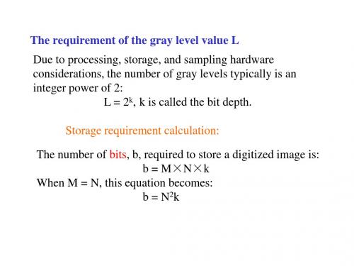
Illustration of histogram equalization
No. of pixels
2 4 3 2
3 2 2 4
3 4 3 2
2 3 5 4
6 5 4 3
2
1
4x4 image Gray scale = [0,9]
Gray level
0 1 2 3 4 5 6 7 8 9
histogram
4-component
4-component
Different ways of measuring distance
1. The Euclidean distance between p and q is defined 1 as: 2 2 2
De ( p, q) [( x s) ( y t ) ]
1 F (u, v) MN
M 1 x 0
M 1 N 1 x 0 y 0
f ( x, y) e
f ( x, y)e
j 2vy/N
j 2 ( ux/M vy/N )
can be expressed in the separable form
1 F (u, v) M
1 0
255=>11111111 235=>11101011 188=>10111100 155=>10011011
0
1
0 1
124=>01111100 90 =>01011010
……
Moving window example: find the minimum
Padded image Original image
Storage requirement calculation:

ASTM材料与实验标准.E94

Designation:E94–04Standard Guide forRadiographic Examination1This standard is issued under theﬁxed designation E94;the number immediately following the designation indicates the year of original adoption or,in the case of revision,the year of last revision.A number in parentheses indicates the year of last reapproval.A superscript epsilon(e)indicates an editorial change since the last revision or reapproval.1.Scope1.1This guide2covers satisfactory X-ray and gamma-ray radiographic examination as applied to industrial radiographic ﬁlm recording.It includes statements about preferred practice without discussing the technical background which justiﬁes the preference.A bibliography of several textbooks and standard documents of other societies is included for additional infor-mation on the subject.1.2This guide covers types of materials to be examined; radiographic examination techniques and production methods; radiographicﬁlm selection,processing,viewing,and storage; maintenance of inspection records;and a list of available reference radiograph documents.N OTE1—Further information is contained in Guide E999,Practice E1025,Test Methods E1030and E1032.1.3Interpretation and Acceptance Standards—Interpretation and acceptance standards are not covered by this guide,beyond listing the available reference radiograph docu-ments for castings and welds.Designation of accept-reject standards is recognized to be within the cognizance of product speciﬁcations and generally a matter of contractual agreement between producer and purchaser.1.4Safety Practices—Problems of personnel protection against X rays and gamma rays are not covered by this document.For information on this important aspect of radiog-raphy,reference should be made to the current document of the National Committee on Radiation Protection and Measure-ment,Federal Register,U.S.Energy Research and Develop-ment Administration,National Bureau of Standards,and to state and local regulations,if such exist.For speciﬁc radiation safety information refer to NIST Handbook ANSI43.3,21 CFR1020.40,and29CFR1910.1096or state regulations for agreement states.1.5This standard does not purport to address all of the safety problems,if any,associated with its use.It is the responsibility of the user of this standard to establish appro-priate safety and health practices and determine the applica-bility of regulatory limitations prior to use.(See1.4.)1.6If an NDT agency is used,the agency shall be qualiﬁed in accordance with Practice E543.2.Referenced Documents2.1ASTM Standards:3E543Practice for Evaluating Agencies that Perform Non-destructive TestingE746Test Method for Determining Relative Image Quality Response of Industrial Radiographic Film SystemsE747Practice for Design,Manufacture,and Material Grouping Classiﬁcation of Wire Image Quality Indicators (IQI)Used for RadiologyE801Practice for Controlling Quality of Radiological Ex-amination of Electronic DevicesE999Guide for Controlling the Quality of Industrial Ra-diographic Film ProcessingE1025Practice for Design,Manufacture,and Material Grouping Classiﬁcation of Hole-Type Image Quality Indi-cators(IQI)Used for RadiologyE1030Test Method for Radiographic Examination of Me-tallic CastingsE1032Test Method for Radiographic Examination of WeldmentsE1079Practice for Calibration of Transmission Densitom-etersE1254Guide for Storage of Radiographs and Unexposed Industrial Radiographic FilmsE1316Terminology for Nondestructive ExaminationsE1390Guide for Illuminators Used for Viewing Industrial RadiographsE1735Test Method for Determining Relative Image Qual-ity of Industrial Radiographic Film Exposed to X-Radiation from4to25MVE1742Practice for Radiographic ExaminationE1815Test Method for Classiﬁcation of Film Systems for Industrial Radiography2.2ANSI Standards:1This guide is under the jurisdiction of ASTM Committee E07on Nondestruc-tive Testing and is the direct responsibility of Subcommittee E07.01on Radiology (X and Gamma)Method.Current edition approved January1,2004.Published February2004.Originally approved st previous edition approved in2000as E94-00.2For ASME Boiler and Pressure Vessel Code applications see related Guide SE-94in Section V of that Code.3For referenced ASTM standards,visit the ASTM website,,or contact ASTM Customer Service at service@.For Annual Book of ASTM Standards volume information,refer to the standard’s Document Summary page on the ASTM website.Copyright©ASTM International,100Barr Harbor Drive,PO Box C700,West Conshohocken,PA19428-2959,United States.PH1.41Speciﬁcations for Photographic Film for Archival Records,Silver-Gelatin Type,on Polyester Base 4PH2.22Methods for Determining Safety Times of Photo-graphic Darkroom Illumination 4PH4.8Methylene Blue Method for Measuring Thiosulfate and Silver Densitometric Method for Measuring Residual Chemicals in Films,Plates,and Papers 4T9.1Imaging Media (Film)—Silver-Gelatin Type Speciﬁ-cations for Stability 4T9.2Imaging Media—Photographic Process Film Plate and Paper Filing Enclosures and Storage Containers 42.3Federal Standards:Title 21,Code of Federal Regulations (CFR)1020.40,Safety Requirements of Cabinet X-Ray Systems 5Title 29,Code of Federal Regulations (CFR)1910.96,Ionizing Radiation (X-Rays,RF,etc.)52.4Other Document:NBS Handbook ANSI N43.3General Radiation Safety Installations Using NonMedical X-Ray and Sealed Gamma Sources up to 10MeV 63.Terminology3.1Deﬁnitions —For deﬁnitions of terms used in this guide,refer to Terminology E 1316.4.Signiﬁcance and Use4.1Within the present state of the radiographic art,this guide is generally applicable to available materials,processes,and techniques where industrial radiographic ﬁlms are used as the recording media.4.2Limitations —This guide does not take into consider-ation special beneﬁts and limitations resulting from the use of nonﬁlm recording media or readouts such as paper,tapes,xeroradiography,ﬂuoroscopy,and electronic image intensiﬁ-cation devices.Although reference is made to documents that may be used in the identiﬁcation and grading,where appli-cable,of representative discontinuities in common metal cast-ings and welds,no attempt has been made to set standards of acceptance for any material or production process.Radiogra-phy will be consistent in sensitivity and resolution only if the effect of all details of techniques,such as geometry,ﬁlm,ﬁltration,viewing,etc.,is obtained and maintained.5.Quality of Radiographs5.1To obtain quality radiographs,it is necessary to consider as a minimum the following list of items.Detailed information on each item is further described in this guide.5.1.1Radiation source (X-ray or gamma),5.1.2V oltage selection (X-ray),5.1.3Source size (X-ray or gamma),5.1.4Ways and means to eliminate scattered radiation,5.1.5Film system class,5.1.6Source to ﬁlm distance,5.1.7Image quality indicators (IQI’s),5.1.8Screens and ﬁlters,5.1.9Geometry of part or component conﬁguration,5.1.10Identiﬁcation and location markers,and 5.1.11Radiographic quality level.6.Radiographic Quality Level6.1Information on the design and manufacture of image quality indicators (IQI’s)can be found in Practices E 747,E 801,E 1025,and E 1742.6.2The quality level usually required for radiography is 2%(2-2T when using hole type IQI)unless a higher or lower quality is agreed upon between the purchaser and the supplier.At the 2%subject contrast level,three quality levels of inspection,2-1T,2-2T,and 2-4T,are available through the design and application of the IQI (Practice E 1025,Table 1).Other levels of inspection are available in Practice E 1025Table 1.The level of inspection speciﬁed should be based on the service requirements of the product.Great care should be taken in specifying quality levels 2-1T,1-1T,and 1-2T by ﬁrst determining that these quality levels can be maintained in production radiography.N OTE 2—The ﬁrst number of the quality level designation refers to IQI thickness expressed as a percentage of specimen thickness;the second number refers to the diameter of the IQI hole that must be visible on the radiograph,expressed as a multiple of penetrameter thickness,T .6.3If IQI’s of material radiographically similar to that being examined are not available,IQI’s of the required dimensions but of a lower-absorption material may be used.6.4The quality level required using wire IQI’s shall be equivalent to the 2-2T level of Practice E 1025unless a higher or lower quality level is agreed upon between purchaser and supplier.Table 4of Practice E 747gives a list of various hole-type IQI’s and the diameter of the wires of corresponding EPS with the applicable 1T,2T,and 4T holes in the plaque IQI.Appendix X1of Practice E 747gives the equation for calcu-lating other equivalencies,if needed.7.Energy Selection7.1X-ray energy affects image quality.In general,the lower the energy of the source utilized the higher the achievable radiographic contrast,however,other variables such as geom-etry and scatter conditions may override the potential advan-tage of higher contrast.For a particular energy,a range of thicknesses which are a multiple of the half value layer,may be radiographed to an acceptable quality level utilizing a particu-lar X-ray machine or gamma ray source.In all cases the speciﬁed IQI (penetrameter)quality level must be shown on the radiograph.In general,satisfactory results can normally be obtained for X-ray energies between 100kV to 500kV in a range between 2.5to 10half value layers (HVL)of material thickness (see Table 1).This range may be extended by as much as a factor of 2in some situations for X-ray energies in the 1to 25MV range primarily because of reduced scatter.4Available from American National Standards Institute (ANSI),25W.43rd St.,4th Floor,New York,NY 10036.5Available from ernment Printing Office Superintendent of Documents,732N.Capitol St.,NW,Mail Stop:SDE,Washington,DC 20401.6Available from National Technical Information Service (NTIS),U.S.Depart-ment of Commerce,5285Port Royal Rd.,Springﬁeld,V A22161.8.Radiographic Equivalence Factors8.1The radiographic equivalence factor of a material is that factor by which the thickness of the material must be multi-plied to give the thickness of a “standard”material (often steel)which has the same absorption.Radiographic equivalence factors of several of the more common metals are given in Table 2,with steel arbitrarily assigned a factor of 1.0.The factors may be used:8.1.1To determine the practical thickness limits for radia-tion sources for materials other than steel,and8.1.2To determine exposure factors for one metal from exposure techniques for other metals.9.Film9.1Various industrial radiographic ﬁlm are available to meet the needs of production radiographic work.However,deﬁnite rules on the selection of ﬁlm are difficult to formulate because the choice depends on individual user requirements.Some user requirements are as follows:radiographic quality levels,exposure times,and various cost factors.Several methods are available for assessing image quality levels (see Test Method E 746,and Practices E 747and E 801).Informa-tion about speciﬁc products can be obtained from the manu-facturers.9.2Various industrial radiographic ﬁlms are manufactured to meet quality level and production needs.Test Method E 1815provides a method for ﬁlm manufacturer classiﬁcation of ﬁlm systems.A ﬁlm system consist of the ﬁlm andassociated ﬁlm processing ers may obtain a classi-ﬁcation table from the ﬁlm manufacturer for the ﬁlm system used in production radiography.A choice of ﬁlm class can be made as provided in Test Method E 1815.Additional speciﬁc details regarding classiﬁcation of ﬁlm systems is provided in Test Method E 1815.ANSI Standards PH1.41,PH4.8,T9.1,and T9.2provide speciﬁc details and requirements for ﬁlm manufacturing.10.Filters10.1Deﬁnition —Filters are uniform layers of material placed between the radiation source and the ﬁlm.10.2Purpose —The purpose of ﬁlters is to absorb the softer components of the primary radiation,thus resulting in one or several of the following practical advantages:10.2.1Decreasing scattered radiation,thus increasing con-trast.10.2.2Decreasing undercutting,thus increasing contrast.10.2.3Decreasing contrast of parts of varying thickness.10.3Location —Usually the ﬁlter will be placed in one of the following two locations:10.3.1As close as possible to the radiation source,which minimizes the size of the ﬁlter and also the contribution of the ﬁlter itself to scattered radiation to the ﬁlm.10.3.2Between the specimen and the ﬁlm in order to absorb preferentially the scattered radiation from the specimen.It should be noted that lead foil and other metallic screens (see 13.1)fulﬁll this function.10.4Thickness and Filter Material —The thickness and material of the ﬁlter will vary depending upon the following:10.4.1The material radiographed.10.4.2Thickness of the material radiographed.10.4.3Variation of thickness of the material radiographed.10.4.4Energy spectrum of the radiation used.10.4.5The improvement desired (increasing or decreasing contrast).Filter thickness and material can be calculated or determined empirically.11.Masking11.1Masking or blocking (surrounding specimens or cov-ering thin sections with an absorptive material)is helpful in reducing scattered radiation.Such a material can also be usedTABLE 1Typical Steel HVL Thickness in Inches [mm]forCommon EnergiesEnergyThickness,Inches [mm]120kV 0.10[2.5]150kV 0.14[3.6]200kV 0.20[5.1]250kV0.25[6.4]400kV (Ir 192)0.35[8.9]1MV0.57[14.5]2MV (Co 60)0.80[20.3]4MV 1.00[25.4]6MV 1.15[29.2]10MV1.25[31.8]16MV and higher1.30[33.0]TABLE 2Approximate Radiographic Equivalence Factors for Several Metals (Relative to Steel)MetalEnergy Level100kV 150kV 220kV 250kV400kV1MV2MV4to 25MV192Ir60CoMagnesium 0.050.050.08Aluminum0.080.120.180.350.35Aluminum alloy 0.100.140.180.350.35Titanium0.540.540.710.90.90.90.90.9Iron/all steels 1.0 1.0 1.0 1.0 1.0 1.0 1.0 1.0 1.0 1.0Copper 1.51.6 1.4 1.41.4 1.1 1.1 1.2 1.1 1.1Zinc 1.4 1.3 1.3 1.2 1.1 1.0Brass 1.4 1.3 1.3 1.2 1.1 1.0 1.1 1.0Inconel X 1.4 1.3 1.3 1.3 1.3 1.3 1.3 1.3Monel 1.7 1.2Zirconium2.4 2.3 2.0 1.7 1.5 1.0 1.0 1.0 1.2 1.0Lead 14.014.012.0 5.0 2.52.7 4.0 2.3Hafnium 14.012.09.03.0Uranium20.016.012.04.03.912.63.4to equalize the absorption of different sections,but the loss of detail may be high in the thinner sections.12.Back-Scatter Protection12.1Effects of back-scattered radiation can be reduced by conﬁning the radiation beam to the smallest practical cross section and by placing lead behind theﬁlm.In some cases either or both the back lead screen and the lead contained in the back of the cassette orﬁlm holder will furnish adequate protection against back-scattered radiation.In other instances, this must be supplemented by additional lead shielding behind the cassette orﬁlm holder.12.2If there is any question about the adequacy of protec-tion from back-scattered radiation,a characteristic symbol (frequently a1⁄8-in.[3.2-mm]thick letter B)should be attached to the back of the cassette orﬁlm holder,and a radiograph made in the normal manner.If the image of this symbol appears on the radiograph as a lighter density than background, it is an indication that protection against back-scattered radia-tion is insufficient and that additional precautions must be taken.13.Screens13.1Metallic Foil Screens:13.1.1Lead foil screens are commonly used in direct contact with theﬁlms,and,depending upon their thickness, and composition of the specimen material,will exhibit an intensifying action at as low as90kV.In addition,any screen used in front of theﬁlm acts as aﬁlter(Section10)to preferentially absorb scattered radiation arising from the speci-men,thus improving radiographic quality.The selection of lead screen thickness,or for that matter,any metallic screen thickness,is subject to the same considerations as outlined in 10.4.Lead screens lessen the scatter reaching theﬁlm regard-less of whether the screens permit a decrease or necessitate an increase in the radiographic exposure.To avoid image unsharp-ness due to screens,there should be intimate contact between the lead screen and theﬁlm during exposure.13.1.2Lead foil screens of appropriate thickness should be used whenever they improve radiographic quality or penetram-eter sensitivity or both.The thickness of the front lead screens should be selected with care to avoid excessiveﬁltration in the radiography of thin or light alloy materials,particularly at the lower kilovoltages.In general,there is no exposure advantage to the use of0.005in.in front and back lead screens below125 kV in the radiography of1⁄4-in.[6.35-mm]or lesser thickness steel.As the kilovoltage is increased to penetrate thicker sections of steel,however,there is a signiﬁcant exposure advantage.In addition to intensifying action,the back lead screens are used as protection against back-scattered radiation (see Section12)and their thickness is only important for this function.As exposure energy is increased to penetrate greater thicknesses of a given subject material,it is customary to increase lead screen thickness.For radiography using radioac-tive sources,the minimum thickness of the front lead screen should be0.005in.[0.13mm]for iridium-192,and0.010in.[0.25mm]for cobalt-60.13.2Other Metallic Screen Materials:13.2.1Lead oxide screens perform in a similar manner to lead foil screens except that their equivalence in lead foil thickness approximates0.0005in.[0.013mm].13.2.2Copper screens have somewhat less absorption and intensiﬁcation than lead screens,but may provide somewhat better radiographic sensitivity with higher energy above1MV.13.2.3Gold,tantalum,or other heavy metal screens may be used in cases where lead cannot be used.13.3Fluorescent Screens—Fluorescent screens may be used as required providing the required image quality is achieved.Proper selection of theﬂuorescent screen is required to minimize image unsharpness.Technical information about speciﬁcﬂuorescent screen products can be obtained from the manufacturers.Goodﬁlm-screen contact and screen cleanli-ness are required for successful use ofﬂuorescent screens. Additional information on the use ofﬂuorescent screens is provided in Appendix X1.13.4Screen Care—All screens should be handled carefully to avoid dents and scratches,dirt,or grease on active surfaces. Grease and lint may be removed from lead screens with a solvent.Fluorescent screens should be cleaned in accordance with the recommendations of the manufacturer.Screens show-ing evidence of physical damage should be discarded.14.Radiographic Image Quality14.1Radiographic image quality is a qualitative term used to describe the capability of a radiograph to showﬂaws in the area under examination.There are three fundamental compo-nents of radiographic image quality as shown in Fig.1.Each component is an important attribute when considering a speciﬁc radiographic technique or application and will be brieﬂy discussed below.14.2Radiographic contrast between two areas of a radio-graph is the difference between theﬁlm densities of those areas.The degree of radiographic contrast is dependent upon both subject contrast andﬁlm contrast as illustrated in Fig.1.14.2.1Subject contrast is the ratio of X-ray or gamma-ray intensities transmitted by two selected portions of a specimen. Subject contrast is dependent upon the nature of the specimen (material type and thickness),the energy(spectral composition, hardness or wavelengths)of the radiation used and the intensity and distribution of scattered radiation.It is independent of time,milliamperage or source strength(curies),source distance and the characteristics of theﬁlm system.14.2.2Film contrast refers to the slope(steepness)of the ﬁlm system characteristic curve.Film contrast is dependent upon the type ofﬁlm,the processing it receives and the amount ofﬁlm density.It also depends upon whether theﬁlm was exposed with lead screens(or without)or withﬂuorescent screens.Film contrast is independent,for most practical purposes,of the wavelength and distribution of the radiation reaching theﬁlm and,hence is independent of subject contrast. For further information,consult Test Method E1815.14.3Film system granularity is the objective measurement of the local density variations that produce the sensation of graininess on the radiographicﬁlm(for example,measured with a densitometer with a small aperture of#0.0039in.[0.1 mm]).Graininess is the subjective perception of a mottled random pattern apparent to a viewer who sees smalllocaldensity variations in an area of overall uniform density (that is,the visual impression of irregularity of silver deposit in a processed radiograph).The degree of granularity will not affect the overall spatial radiographic resolution (expressed in line pairs per mm,etc.)of the resultant image and is usually independent of exposure geometry arrangements.Granularity is affected by the applied screens,screen-ﬁlm contact and ﬁlm processing conditions.For further information on detailed perceptibility,consult Test Method E 1815.14.4Radiographic deﬁnition refers to the sharpness of the image (both the image outline as well as image detail).Radiographic deﬁnition is dependent upon the inherent un-sharpness of the ﬁlm system and the geometry of the radio-graphic exposure arrangement (geometric unsharpness)as illustrated in Fig.1.14.4.1Inherent unsharpness (U i )is the degree of visible detail resulting from geometrical aspects within the ﬁlm-screen system,that is,screen-ﬁlm contact,screen thickness,total thickness of the ﬁlm emulsions,whether single or double-coated emulsions,quality of radiation used (wavelengths,etc.)and the type of screen.Inherent unsharpness is independent of exposure geometry arrangements.14.4.2Geometric unsharpness (U g )determines the degree of visible detail resultant from an “in-focus”exposure arrange-ment consisting of the source-to-ﬁlm-distance,object-to-ﬁlm-distance and focal spot size.Fig.2(a)illustrates these condi-tions.Geometric unsharpness is given by the equation:U g 5Ft /d o(1)where:U g =geometric unsharpness,F =maximum projected dimension of radiation source,t =distance from source side of specimen to ﬁlm,and d o =source-object distance.N OTE 3—d o and t must be in the same units of measure;the units of U g will be in the same units as F .N OTE 4—A nomogram for the determination of U g is given in Fig.3(inch-pound units).Fig.4represents a nomogram in metric units.Example:Given:Source-object distance (d o )=40in.,Source size (F)=500mils,andSource side of specimen to ﬁlm distance (t)=1.5in.Draw a straight line (dashed in Fig.3)between 500mils on the F scale and 1.5in.on the t scale.Note the point on intersection (P)of this line with the pivot line.Draw a straight line (solid in Fig.3)from 40in.on the d o scale through point P and extend to the U g scale.Intersection of this line with the U g scale gives geometrical unsharpness in mils,which in the example is 19mils.Inasmuch as the source size,F ,is usually ﬁxed for a given radiation source,the value of U g is essentially controlled by the simple d o /t ratio.Geometric unsharpness (U g )can have a signiﬁcant effect on the quality of the radiograph;therefore source-to-ﬁlm-distance (SFD)selection is important.The geometric unsharpness (U g )equation,Eq 1,is for information and guidance and provides a means for determining geometric unsharpness values.The amount or degree of unsharpness should be minimized when establishing the radiographic technique.Radiographic Image QualityRadiographic ContrastFilm System Granularity Radiographic DeﬁnitionSubject Contrast Film Contrast •Grain size and distribution within the ﬁlm emulsion •Processing conditions(type and activity of developer,temperature of developer,etc.)•Type ofscreens (that is,ﬂuorescent,lead or none)•Radiation quality (that is,energy level,ﬁltration,etc.•Exposure quanta (that is,intensity,dose,etc.)InherentUnsharpness Geometric Unsharpness Affected by:•Absorption differences in specimen (thickness,composition,density)•Radiation wavelength •Scattered radiationAffected by:•Type of ﬁlm•Degree of development (type of developer,time,temperature and activity of developer,degree of agitation)•Film density •Type ofscreens (that is,ﬂuorescent,lead or none)Affected by:•Degree of screen-ﬁlm contact •Total ﬁlm thickness •Single ordouble emulsion coatings •Radiation quality •Type and thickness of screens (ﬂuorescent,lead or none)Affected by:•Focal spot or source physical size •Source-to-ﬁlm distance •Specimen-to-ﬁlm distance•Abruptness of thickness changes in specimen •Motion of specimen or radiation sourceReduced or enhanced by:•Masks and diaphragms •Filters•Lead screens •Potter-Bucky diaphragmsFIG.1Variables of Radiographic ImageQualityFIG.2Effects of Object-Film Geometry15.Radiographic Distortion15.1The radiographic image of an object or feature within an object may be larger or smaller than the object or feature itself,because the penumbra of the shadow is rarely visible in a radiograph.Therefore,the image will be larger if the object or feature is larger than the source of radiation,and smaller if object or feature is smaller than the source.The degree of reduction or enlargement will depend on the source-to-object and object-to-ﬁlm distances,and on the relative sizes of the source and the object or feature (Fig.2(b )and (c )).15.2The direction of the central beam of radiation should be perpendicular to the surface of the ﬁlm whenever possible.The object image will be distorted if the ﬁlm is not aligned perpendicular to the central beam.Different parts of the object image will be distorted different amount depending on the extent of the ﬁlm to central beam offset (Fig.2(d )).16.Exposure Calculations or Charts16.1Development or procurement of an exposure chart or calculator is the responsibility of the individual laboratory.16.2The essential elements of an exposure chart or calcu-lator must relate the following:16.2.1Source or machine,16.2.2Material type,16.2.3Material thickness,16.2.4Film type (relative speed),16.2.5Film density,(see Note 5),16.2.6Source or source to ﬁlm distance,16.2.7Kilovoltage or isotope type,N OTE 5—For detailed information on ﬁlm density and density measure-ment calibration,see Practice E 1079.16.2.8Screen type andthickness,FIG.3Nomogram for Determining Geometrical Unsharpness (Inch-PoundUnits)16.2.9Curies or milliampere/minutes,16.2.10Time of exposure,16.2.11Filter (in the primary beam),16.2.12Time-temperature development for hand process-ing;access time for automatic processing;time-temperature development for dry processing,and16.2.13Processing chemistry brand name,if applicable.16.3The essential elements listed in 16.2will be accurate for isotopes of the same type,but will vary with X-ray equipment of the same kilovoltage and milliampere rating.16.4Exposure charts should be developed for each X-ray machine and corrected each time a major component is replaced,such as the X-ray tube or high-voltage transformer.16.5The exposure chart should be corrected when the processing chemicals are changed to a different manufacturer’s brand or the time-temperature relationship of the processormay be adjusted to suit the exposure chart.The exposure chart,when using a dry processing method,should be corrected based upon the time-temperature changes of the processor.17.Technique File17.1It is recommended that a radiographic technique log or record containing the essential elements be maintained.17.2The radiographic technique log or record should con-tain the following:17.2.1Description,photo,or sketch of the test object illustrating marker layout,source placement,and ﬁlm location.17.2.2Material type and thickness,17.2.3Source to ﬁlm distance,17.2.4Film type,17.2.5Film density,(see Note 5),17.2.6Screen type andthickness,FIG.4Nomogram for Determining Geometrical Unsharpness (MetricUnits)。

latex编译技巧

Optimization Methods and SoftwareVol.00,No.00,January2009,1–18GUIDEOptimization Methods and Software—L A T E X2εstyle guide for authors(Style2+References Style S)Taylor&Francis a∗and I.T.Consultant ba4Park Square,Milton Park,Abingdon,OX144RN,UK;b Institut f¨u r Informatik, Albert-Ludwigs-Universit¨a t,D-79110Freiburg,Germany(v4.4released October2008)This guide is for authors who are preparing papers for the Taylor&Francis journal Optimiza-tion Methods and Software(gOMS)using the L A T E X2εdocument preparation system and the Classﬁle gOMS2e.cls,which is available via the journal homepage on the Taylor&Francis website(see Section8).Authors planning to submit their papers in L A T E X2εare advised to use gOMS2e.cls as early as possible in the creation of theirﬁles.Keywords:submission instructions;sourceﬁle coding;environments;references citation;fonts;numbering(Authors:Please provide three to six keywords taken from terms used in your manuscript)AMS Subject Classiﬁcation:F1.1;F4.3(...for example;authors are encouragedto provide two to six AMS Subject Classiﬁcation codes)Index to information contained in this guide1.Introduction1.1.The gOMS document style1.2.Submission of L A T E X2εarticlesto the journaling the gOMS Classﬁlendscape pages3.Additional features3.1.Footnotes to article titlesand authors’names3.2.Abstracts3.3.Lists4.Some guidelines for usingstandard features4.1.Sections4.2.Illustrations(ﬁgures)4.3.Tables4.4.Running headlines4.5.Maths environments4.6.Typesetting mathematics4.6.1.Displayed mathematics4.6.2.Bold math italic symbols4.6.3.Bold Greek4.6.4.Upright lowercase Greek characters4.7.Acknowledgements4.8.Notes4.9.Appendices4.10.References4.10.1.References cited in thetext4.10.2.The list of references4.11.gOMS macros5.Example of a section heading with small caps,lowercase,italic,and bold Greek such asκ6.gOMS journal style6.1.Punctuation6.2.Spelling6.3.Hyphens,n-rules,m-rules andminus signs6.4.References6.5.Maths fonts7.Troubleshooting7.1.Fixes for coding problems8.Obtaining the gOMS2e Classﬁle8.1Via the Taylor&Francis website8.2Via e-mailPlease note that the index following the abstract in this guide is provided for information only.An index is not required in submitted papers.∗Corresponding author.Email:latex.helpdesk@ISSN:1055-6788print/ISSN1029-4937onlinec 2009Taylor&FrancisDOI:10.1080/1055678xxxxxxxxxxxxx2Taylor&Francis and I.T.Consultant1.IntroductionAuthors are encouraged to submit manuscripts to Optimization Methods and Soft-ware(gOMS)electronically.Electronic submissions should be sent as e-mail at-tachments using a standard word processing program,such as Microsoft Word or PDF created from L A T E X2εsourceﬁles(see Section1.2).gOMS does not accept Microsoft Word2007documents.Please use Word’s‘Save As’option to save your document as an older(.doc)ﬁle type.If e-mail submission is not possible,please send an electronic version on disc.The layout design for gOMS has been implemented as a L A T E X2εClassﬁle.The gOMS Classﬁle is based on mands that diﬀer from the standard L A T E X2εinterface,or which are provided in addition to the standard interface,are explained in this guide.This guide is not a substitute for the L A T E X2εmanual itself.This guide can be used as a template for composing an article for submission by cutting,pasting,inserting and deleting text as appropriate,using the LaTeX environments provided(e.g.\begin{equation},\begin{corollary}).1.1.The gOMS document styleThe use of L A T E X2εdocument styles allows a simple change of style(or style option) to transform the appearance of your document.The gOMS2e Classﬁle preserves the standard L A T E X2εinterface such that any document that can be produced using the standard L A T E X2εarticle style can also be produced with the gOMS style. However,the measure(or width of text)is narrower than the default for article, therefore line breaks will change and long equations may need re-formatting. When your article appears in the print edition of the gOMS journal,it is typeset in Monotype Times.As most authors do not own this font,it is likely that the page make-up will change with the change of font.For this reason,we ask you to ignore details such as slightly long lines,page stretching,orﬁgures falling out of synchronization with their citations in the text,because these details will be dealt with at a later stage.1.2.Submission of L A T E X2εarticles to the journalSubmissions to be considered for publication in Optimization Methods and Soft-ware should be sent to the appropriate Editor at one of the following addresses: O.Burdakov(Co-Editor),Division of Optimization,Department of Mathemat-ics,Link¨o ping University,58183Link¨o ping,Sweden(e-mail:burdakov@mai.liu.se);A.Griewank(Co-Editor),Humboldt University Berlin,Mat Nat Faculty II, Department of Mathematics,Unter den Linden6,10099Berlin,Germany(e-mail:griewank@mathematik.hu-berlin.de);T.Tsuchiya(Regional Editor,Asia), The Institute of Statistical Mathematics,4-6-7Minami-Azabu,Minato-ku,Tokyo 106-8569,Japan(e-mail:tsuchiya@sun312.ism.ac.jp);S.Ulbrich(Regional Edi-tor,Europe),Technische Universit¨a t Darmstadt,Fachbereich Mathematik,AG10, Schloßgartenstr.7,64289Darmstadt,Germany(e-mail:ulbrich@mathematik.tu-darmstadt.de);F.A.Potra(Regional Editor,Americas),Department of Mathe-matics and Statistics,University of Maryland,Baltimore,MD21250,USA(e-mail: potra@);or M.Anitescu(Software Editor),Mathematics and Com-puter Science,Argonne National Laboratory,9700South Cass Avenue,Argonne, IL60439-4844,USA(e-mail:anitescu@).Optimization Methods and Software3 Authors are encouraged to submit manuscripts electronically.If e-mail submis-sion is not possible,please send an electronic version on disc.General Instructions for Authors may be found at (/journals/authors/gomsauth.asp).Only‘open-source’L A T E X2εshould be used,not proprietary systems such as TCI LaTeX or Scientiﬁc WorkPlace.Similarly,Classﬁles such as REVTex4that produce a document in the style of a diﬀerent publisher and journal should not be used for preference.Appropriate gaps should be left forﬁgures,for which original electronicﬁles should be supplied.Authors should ensure that theirﬁgures are suitable(in terms of lettering size,etc.)for the reductions they intend.Authors who wish to incorporate Encapsulated PostScript artwork directly in their articles can do so by using Tomas Rokicki’s EPSF macros(which are supplied with the DVIPS PostScript driver).See Section2.1,which also demonstrates how to treat landscape pages.Please remember to supply any additionalﬁgure macros you use with your article in the preamble before begin{document}.Authors should not attempt to use implementation-speciﬁc\special’s directly.Ensure that any author-deﬁned macros are gathered together in the sourceﬁle, just before the\begin{document}command.Please note that,if serious problems are encountered with the coding of a paper (missing author-deﬁned macros,for example),it may prove necessary to divert the paper to conventional typesetting,i.e.it will be re-keyed.ing the gOMS ClassﬁleIf theﬁle gOMS2e.cls is not already in the appropriate system directory for L A T E X2εﬁles,either arrange for it to be put there,or copy it to your working folder.The gOMS document style is implemented as a complete document style, not a document style option.In order to use the gOMS style,replace‘article’by ‘gOMS2e’in the\documentclass command at the beginning of your document: \documentclass{article}is replaced by\documentclass{gOMS2e}In general,the following standard document style options should not be used with the gOMS style:(1)10pt,11pt,12pt—unavailable;(2)oneside(no associated styleﬁle)—oneside is the default;(3)leqno and titlepage—should not be used;(4)singlecolumn—is not necessary as it is the default style.ndscape pagesIf a table or illustration is too wide toﬁt the standard measure,it must be turned,with its caption,through90◦ndscape illustra-tions and/or tables can be produced directly using the gOMS2e styleﬁle us-ing\usepackage{rotating}after\documentclass{gOMS2e}.The following com-mands can be used to produce such pages.\setcounter{figure}{2}\begin{sidewaysfigure}4Taylor&Francis and I.T.Consultant\centerline{\epsfbox{fig1.eps}}\caption{This is an example of figure caption.}\label{landfig}\end{sidewaysfigure}\setcounter{table}{0}\begin{sidewaystable}\tbl{The Largest Optical Telescopes.}\begin{tabular}{@{}llllcll}...\end{tabular}\label{tab1}\end{sidewaystable}Before anyﬂoat environment,use the\setcounter command as above toﬁx the numbering of the caption.Subsequent captions will then be automatically renum-bered accordingly.3.Additional featuresIn addition to all the standard L A T E X2εdesign elements,gOMS style includes a separate command for specifying short versions of the authors’names and the journal title for running headlines on the left-hand(verso)and right-hand(recto) pages,respectively(see Section4.4).In general,once you have used this additional gOMS2e.cls feature in your document,do not process it with a standard L A T E X2εstyleﬁle.3.1.Footnotes to article titles and authors’namesOn the title page,the\thanks command may be used to produce a footnote to either the title or authors’names.Footnote symbols should be used in the order:†(coded as\dagger),‡(\ddagger),§(\S),¶(\P), (\|),††(\dagger\dagger),‡‡(\ddagger\ddagger),§§(\S\S),¶¶(\P\P), (\|\|).Note that footnotes to the text will automatically be assigned the superscript symbols1,2,3,...by the Classﬁle,beginning afresh on each page.1The title,author(s)and aﬃliation(s)should be followed by the\maketitle com-mand.3.2.AbstractsAt the beginning of your article,the title should be generated in the usual way using the\maketitle command.Immediately following the title you should include an abstract.The abstract should be enclosed within an abstract environment.For example,the titles for this guide were produced by the following source code:\title{Optimization Methods and Software:\LaTeXe\style%1These symbols will be changed to the style of the journal by the typesetter during preparation of your proofs.Optimization Methods and Software5guide for authors}\author{Taylor\&Francis Limited,4Park Square,Milton Park,Abingdon,OX144RN,UK}\received{v4.4released October2008} \maketitle\begin{abstract}This guide is for authors who are preparing papers for the Taylor\&% Francis journal{\em Optimization Methods and Software}%({\it gOMS}\,)using the\LaTeXe\document preparation system and%the Class file{\tt gOMS2e.cls},which is available via the journal% homepage on the Taylor\&Francis website(see Section~\ref{FTP}).% Authors planning to submit their papers in\LaTeXe\are advised to%use{\tt gOMS2e.cls}as early as possible in the creation of their%files.\end{abstract}(Please note that the percentage signs at the ends of lines that quote source code in this document are not part of the coding but have been inserted to achieve line wrapping at the appropriate points.)3.3.ListsThe gOMS style provides numbered and unnumbered lists using the enumerate environment and bulleted lists using the itemize environment.The enumerated list numbers each list item with arabic numerals:(1)ﬁrst item(2)second item(3)third itemAlternative numbering styles can be achieved by inserting a redeﬁnition of the number labelling command after the\begin{enumerate}.For example,the list(i)ﬁrst item(ii)second item(iii)third itemwas produced by:\begin{enumerate}\item[(i)]first item\item[(ii)]second item\item[(iii)]third item\end{enumerate}Unnumbered lists are also provided using the enumerate environment.For example, First unnumbered indented item without label.Second unnumbered item.Third unnumbered item.was produced by:\begin{enumerate}\item[]First unnumbered indented item...6Taylor&Francis and I.T.Consultant\item[]Second unnumbered item.\item[]Third unnumbered item.\end{enumerate}Bulleted lists are provided using the itemize environment.For example,•First bulleted item•Second bulleted item•Third bulleted itemwas produced by:\begin{itemize}\item First bulleted item\item Second bulleted item\item Third bulleted item\end{itemize}4.Some guidelines for using standard featuresThe following notes may help you achieve the best eﬀects with the gOMS2e Class ﬁle.4.1.SectionsL A T E X2εprovidesﬁve levels of section headings and they are all deﬁned in the gOMS2e Classﬁle:(1)\section(2)\subsection(3)\subsubsection(4)\paragraph(5)\subparagraphNumbering is automatically generated for section,subsection,subsubsection and paragraph headings.If you need additional text styles in the headings,see the examples in Section5.4.2.Illustrations(ﬁgures)The gOMS style will cope with most positioning of your illustrations and you should not normally use the optional positional qualiﬁers of the figure environ-ment,which would override these decisions.See‘Instructions for Authors’in the journal’s homepage on the Taylor&Francis website for how to submit artwork (/journals/authors/gomsauth.asp).Figure captions should be below theﬁgure itself,therefore the\caption command should appear after theﬁgure.For example,Figure1with caption and sub-captions is produced using the following commands:\begin{figure}\begin{center}\subfigure[]{\resizebox*{5cm}{!}{\includegraphics{senu_gr1.eps}}}%\subfigure[]{\resizebox*{5cm}{!}{\includegraphics{senu_gr2.eps}}}%Optimization Methods and Software7(a)(b)Figure1.Example of a two-partﬁgure with individual sub-captions showingthat all lines ofﬁgure captions range left.Table1.Radio-band beaming model parameters for FSRQsand BL Lacs.Class aγ1γ2b γ G fθcBL Lacs5367−4.01.0×10−210◦FSRQs54011−2.30.5×10−214◦a This is not as accurate,owing to numerical error.b An example table footnote to show the text turning overwhen a long footnote is inserted.\caption{\label{fig2}Example of a two-part figure with individual% sub-captions showing that all lines of figure captions range left.}% \label{sample-figure}\end{center}\end{figure}The control sequences\epsfig{},\subfigure{}and\includegraphics{}re-quire epsﬁg.sty,subﬁgure.sty and graphicx.sty.These are called by the Classﬁle gOMS2e.cls and are included with the LaTeX package for this journal for conve-nience.To ensure thatﬁgures are correctly numbered automatically,the\label{}com-mand should be inserted just after\caption{}4.3.TablesThe gOMS style will cope with most positioning of your tables and you should not normally use the optional positional qualiﬁers of the table environment,which would override these decisions.The table caption appears above the body of the table in gOMS style,therefore the\tbl command should appear before the body of the table.The tabular environment can be used to produce tables with single thick and thin horizontal rules,which are allowed,if desired.Thick rules should be used at the head and foot only and thin rules elsewhere.Commands to redeﬁne quantities such as\arraystretch should be omitted. For example,table1is produced using the following commands.Note that\rm will produce a roman character in math mode.There are also\bf and\it,which produce bold face and text italic in math mode.\begin{table}\tbl{Radio-band beaming model parameters8Taylor&Francis and I.T.Consultantfor{FSRQs and BL Lacs.}}{\begin{tabular}{@{}lcccccc}\topruleClass$^{\rm a}$&$\gamma_1$&$\gamma_2$$^{\rm b}$&$\langle\gamma\rangle$&$G$&$f$&$\theta_{c}$\\\colruleBL Lacs&5&36&7&$-4.0$&$1.0\times10^{-2}$&10$^\circ$\\FSRQs&5&40&11&$-2.3$&$0.5\times10^{-2}$&14$^\circ$\\\botrule\end{tabular}}\tabnote{$^{\rm a}$This is not as accurate,owing tonumerical error.}\tabnote{$^{\rm b}$An example table footnote to show thetext turning over when a long footnote is inserted.}%\label{symbols}\end{table}To ensure that tables are correctly numbered automatically,the\label{}com-mand should be inserted just before\end{table}.4.4.Running headlinesIn gOMS style,the authors’names and the title of the journal are used throughout the article as running headlines at the top of alternate pages. An abbreviated list of authors’names in italic format appears on even-numbered pages(versos)—e.g.‘J.Smith and P.Jones’,or‘J.Smith et al.’for three or more authors—and the journal title in italic format is used on odd-numbered pages(rectos).To achieve this,the\markboth command is used.The running headlines for this guide were produced using the following code:\markboth{Taylor\&Francis and I.T.Consultant}{Optimization Methods and Software}.The\pagestyle and\thispagestyle commands should not be used.4.5.Maths environmentsThe gOMS style provides for the following maths environments.Lemma4.1More recent algorithms for solving the semideﬁnite programming relax-ation are particularly eﬃcient,because they explore the structure of the MAX-CUT.Theorem4.2More recent algorithms for solving the semideﬁnite programming relaxation are particularly eﬃcient,because they explore the structure of the MAX-CUT.Corollary4.3More recent algorithms for solving the semideﬁnite programming relaxation are particularly eﬃcient,because they explore the structure of the MAX-CUT.Proposition4.4More recent algorithms for solving the semideﬁnite programming relaxation are particularly eﬃcient,because they explore the structure of the MAX-CUT.Optimization Methods and Software9 Proof More recent algorithms for solving the semideﬁnite programming relaxation are particularly eﬃcient,because they explore the structure of the MAX-CUT.Remark1More recent algorithms for solving the semideﬁnite programming relax-ation are particularly eﬃcient,because they explore the structure of the MAX-CUT problem.Algorithm1More recent algorithms for solving the semideﬁnite programming re-laxation are particularly eﬃcient,because they explore the structure of the MAX-CUT problem.These were produced by:\begin{lemma}More recent algorithms for solving the semidefiniteprogramming relaxation are particularly efficient,because they explore the structure of the MAX-CUT.\end{lemma}\begin{theorem}......\end{theorem}\begin{corollary}......\end{corollary}\begin{proposition}......\end{proposition}\begin{proof}......\end{proof}\begin{remark}......\end{remark}\begin{algorithm}......\end{algorithm}10Taylor&Francis and I.T.Consultant4.6.Typesetting mathematics4.6.1.Displayed mathematicsThe gOMS style will set displayed mathematics centred on the measure without equation numbers,provided that you use the L A T E X2εstandard control sequences open(\[)and close(\])square brackets as delimiters.The equationpλi=trace(S)i∈Ri=1was typeset in the gOMS style using the commands\[\sum_{i=1}^p\lambda_i={\rm trace}({\textrm{\bf S}})\qquadi\in{\mathbb R}\].For those of your equations that you wish to be automatically numbered sequen-tially throughout the text,use the equation environment,e.g.pλi=trace(S)i∈R(1)i=1was typeset using the commands\begin{equation}\sum_{i=1}^p\lambda_i={\rm trace}({\textrm{\bf S}})quadi\in{\mathbb R}\end{equation}Part numbers for sets of equations may be generated using the subequations environment,e.g.ερw tt(s,t)=N[w s(s,t),w st(s,t)]s,(2a)w tt(1,t)+N[w s(1,t),w st(1,t)]=0,(2b) which was generated using the control sequences\begin{subequations}\label{subeqnexample}\begin{equation}\varepsilon\rho w_{tt}(s,t)=N[w_{s}(s,t),w_{st}(s,t)]_{s},\label{subeqnpart}\end{equation}\begin{equation}w_{tt}(1,t)+N[w_{s}(1,t),w_{st}(1,t)]=0,\end{equation}\end{subequations}This is made possible by the package subeqn,which is called by the Classﬁle.If you put the\label{}just after the\begin{subequations}line,references will be to the collection of equations,‘(2)’in the example above.Or,like the example code above,you can reference each equation individually—e.g.‘(2a)’.4.6.2.Bold math italic symbolsTo get bold math italic you can use\bm,which works for all sizes,e.g.\sffamily\begin{equation}{\rm d}({\bm s_{t_{\bm u}})=\langle{\bm\alpha({\sf{\textbf L}})}% [RM({\bm X}_y+{\bm s}_t)-RM({\bm x}_y)]^2\rangle.\end{equation}\normalfontproduces)= α(L)[RM(X y+s t)−RM(x y)]2 .(3)d(s tuNote that subscript,superscript,subscript to subscript,etc.sizes will take care of themselves and are italic,not bold,unless coded individually.\bm produces the same eﬀect as\boldmath.\sffamily...\normalfont allows upright sans serif fonts to be created in math mode by using the control sequence‘\sf’.4.6.3.Bold GreekBold lowercase as well as uppercase Greek characters can be obtained by {\bm\gamma},which givesγ,and{\bm\Gamma},which givesΓ.4.6.4.Upright lowercase Greek characters and the upright partial derivative sign Upright lowercase Greek characters can be obtained with the Classﬁle by insert-ing the letter‘u’in the control code for the character,e.g.\umu and\upi produce µ(used,for example,in the symbol for the unit microns—µm)andπ(the ratio of the circumference to the diameter of a circle).Similarly,the control code for the upright partial derivative∂is\upartial.4.7.AcknowledgementsAn unnumbered section,e.g.\section*{Acknowledgement(s)},should be used for thanks,grant details,etc.and placed before any Notes or References sections.4.8.NotesAn unnumbered section,e.g.\section*{Note(s)},may be inserted after any Ac-knowledgements and before any References section.4.9.AppendicesAppendices should be set after the references,beginning with the command \appendices followed by the command\section for each appendix title,e.g.\appendices\section{This is the title of the first appendix}\section{This is the title of the second appendix}producesAppendix A.This is the title of theﬁrst appendixAppendix B.This is the title of the second appendixSubsections,equations,theorems,ﬁgures,tables,etc.within appendices will then be automatically numbered as appropriate.4.10.References4.10.1.References cited in the textReferences cited in the text should be quoted by their number as they are listed in the alphabetical References list towards the end of the document, not the order of citation,so theﬁrst reference cited in the text might be [23].For example,these may take the forms[32],[5,6,14],[21–55](not[21]–[55]).To produce the References list,the bibliographic data about each refer-ence item should be listed in thebibliography environment in alphabetical or-der.Each bibliographical entry has a key,which is assigned by the author and used to refer to that entry in the text.In this document,the key glov00in the citation form\cite{glov00}produces‘[5]’,and the keys ed84and aiex02 in the citation form\cite{ed84,aiex02}produce‘[1,3]’.The citation for a range of bibliographic entries(e.g.‘[2,4,6–10]’)will automatically be produced by\cite{doniz00,fzf88,GHGsoft,lam86,mtw73,neu83,fwp88}.Optional notes may be included at the end of a citation by the use of square brackets, e.g. \cite[see][and references therein]{fzf88}produces‘[see4,and references therein]’.4.10.2.The list of referencesThe following listing shows some references prepared in the style of the journal; note that references having the same author(s)are listed chronologically,beginning with the earliest.References[1]R.M.Aiex,Conjectured statistics for the q,t-Catalan numbers,preprint(2002),to appear in Advancesin Math.Available at /∼rmaiex.[2]G.Donizetti,C.M.von Weber,et,C.P.E.Bach,R.Strauss,and L.van Beethoven,Computingtools for modelling orchestral performance,Tech.Rep.DAMTP2000/NA10,Department of Applied Mathematics and Theoretical Physics,University of Cambridge,Cambridge,UK,2000.[3] D.M.F.Edwards and I.R.McDonald,Positive bases in numerical optimization,Comput.Optim.Appl.21(1984),pp.169–175.[4] F.French,English title of a chapter in the translation of a book in a foreign language,in Title ofa Book in Another Language(Quoted in that Language)[English translation],P.Smith(Transl.),Dover,New York(1988),original work published1923.[5] F.Glover,Multi-start and strategic oscillation methods—principles to exploit adaptive memory,inComputing Tools for Modeling,Optimization and Simulation:Interfaces in Computer Science and Operations Research,guna and J.L.Gonz´a les-Velarde,eds.,2nd ed.,Vol.6,Kluwer Academic, Boston,MA,2000,pp.1–24.[6]T.G.Golda,P.D.Hough,and G.Gay,APPSPACK(Asynchronous parallel pattern search package);software available at /appspack.[7]mport,Hilbert modular forms and the Galois representations associated to Hilbert–Blumenthalabelian varieties,Ph.D.diss.,School of Engineering and Applied Sciences,Harvard University,Cam-bridge,MA,1986.[8] C.W.Misner(ed.),Nonlinear Operators and Nonlinear Equations of Evolution in Banach Spaces,Proceedings of Symposia in Pure Mathematics Vol.18,Part2,American Mathematical Society, Providence,RI,1973,pp.231–256.[9]M.Neumann,Parallel GRASP with path-relinking for job shop scheduling,Mol.Phys.50(1983),pp.841–843.[10] F.W.Patel,Title of a Book,Monographs on Technical Aspects Vol.II,Dover,New York,1988.[11]H.Quorn,The resurgent Japanese economy and a Japan–United States free trade agreement,in4thInternational Conference on the Restructuring of the Economic and Political System in Japan andEurope,Milan,Italy,21–25May1996,World Scientiﬁc,Singapore,1997,pp.147–156.This list was produced by:\begin{thebibliography}{12}\bibitem[1]{aiex02}%1R.M.Aiex,{\em Conjectured statistics for the{$q,t$}-Catalan%numbers},preprint(2002),to appear in Advances in Math.Available%at /$\sim$rmaiex.\bibitem[2]{doniz00}%2G.Donizetti, C.M.{{v}on~Weber},et,C.P.E.Bach,R.Strauss,%and L.{{v}an~Beethoven},{\em Computing tools for modelling orchestral% performance},Tech.Rep.DAMTP2000/NA10,Department of Applied%Mathematics and Theoretical Physics,University of Cambridge,Cambridge,%UK,2000.\bibitem[3]{ed84}%3D.M.F.Edwards and I.R.McDonald,{\em Positive bases in numerical% optimization},Comput.Optim.Appl.21(1984),pp.169--175.\bibitem[4]{fzf88}%4F.French,{\em{English title of a chapter in the translation of a%book in a foreign language}},in{\itshape Title of a Book in Another%Language(Quoted in that Language)}[{\itshape English translation}],%P.Smith(Transl.),Dover,New York(1988),original work published1923.\bibitem[5]{glov00}%5F.Glover,{\it{Multi-start and strategic oscillation methods---principles%to exploit adaptive memory}},in{\it Computing Tools for Modeling,%Optimization and Simulation:Interfaces in Computer Science and Operations% Research},guna and J.L.Gonz\’{a}les-Velarde,eds.,2nd ed.,Vol.6,Kluwer% Academic,Boston,MA,2000,pp.1--24.\bibitem[6]{GHGsoft}%6T.G.Golda,P.D.Hough,and G.Gay,{\em{APPSPACK(Asynchronous parallel pattern% search package);}}software available at /appspack.\bibitem[7]{lam86}%7mport,{\em Hilbert modular forms and the Galois representations%associated to Hilbert--Blumenthal abelian varieties},Ph.D.diss.,School of% Engineering and Applied Sciences,Harvard University,Cambridge,MA,1986.\bibitem[8]{mtw73}%8C.W.Misner(ed.),{\em{Nonlinear Operators and Nonlinear Equations of Evolution% in Banach Spaces}},Proceedings of Symposia in Pure Mathematics Vol.18,Part%2,American Mathematical Society,Providence,RI,1973,pp.231--256.\bibitem[9]{neu83}%9M.Neumann,{\em Parallel GRASP with path-relinking for job shop%scheduling},Mol.Phys.50(1983),pp.841--843.。

RCS1

Extraction of Virtual Scattering Centers of Vehicles by Ray-Tracing SimulationsKarin Schuler,Denis Becker,and Werner Wiesbeck,Fellow,IEEEAbstract—Radar images of complex targets can be understood as a superposition of the reﬂected signals from a high number of scattering centers.To model complex targets for radar simulations, the plurality of scattering centers should be reduced to few signiﬁ-cant scattering centers in order to minimize computational effort. The scope of this work is to present a technique to generate a signif-icantly simpliﬁed RCS model of the vehicle with a limited number of virtual scattering centers,each with its own scattering charac-teristic,and how to group these scattering centers in a cluster data-base.The work is based on ray-tracing simulations of complex vehicle models.The ray-tracing simulations have been validated by measurements.The scattering centers may not be physically existing strong scattering centers,but virtual scattering centers representing a certain scattering behavior.In this paper,a tech-nique for extracting such virtual scattering centers from a complex 3D-vehicle-model is presented.It is based on ray-tracing simula-tions of such models.As an example,the design model of a Ford Focus is used.Index Terms—Ray-tracing,RCS-modeling,scattering center.I.I NTRODUCTIOND URING the last years,safety relevant sensor systems havebecome an important feature in the automotive industry. Presently,short range radar(SRR)systems are being devel-oped and introduced to the market.Their intention is to cover the near surrounding of a vehicle to assist the driver during Stop-n-Go trafﬁc and parking,but also to increase safety by blind-spot surveillance and side impact warnings.Currently,dif-ferent approaches are being discussed for the realization of a radar sensor with full azimuth coverage and high azimuth res-olution of the close-by environment.To simulate and evaluate the performance of different approaches for such SRR-systems, scattering-models of vehicles are required.Since vehicles ob-served in the close-by region exhibit multiple scattering centers, contributions from different angles are expected.Depending on the incidence angle,they cause multiple intensity maxima in radar images[1].By describing the scattering characteristics of complex objects by one single RCS value,the multiple scat-tering centers and other scattering phenomena are not apparentManuscript received January22,2007;revised July12,2008.Current version published November14,2008.K.Schuler was with the Universität Karlsruhe(TH),Institut für Höch-stfrequenztechnik und Eletronik(IHE),Karlsruhe D76131,Germany.She is now with EADS Defence Electronics,Ulm D89077,Germany(e-mail: karin.schuler@a.de).D.Becker and W.Wiesbeck are with the Universität Karlsruhe(TH),Institut für Höchstfrequenztechnik und Eletronik(IHE),Karlsruhe D76131,Germany (e-mail:denis.becker@a.de;werner.wiesbeck@a.de).Color versions of one or more of theﬁgures in this paper are available at .Digital Object Identiﬁer10.1109/TAP.2008.2005436anymore.For this reason,it is not sufﬁcient to consider a single scattering center or an azimuth independent RCS in the simu-lations.However,the multiple scattering centers are important and have to be taken into account in radar imaging simulations with high azimuth resolution.A scattering center description for target recognition in one dimension is proposed in[2].Ap-proaches for scattering center extraction are suggested in[3], [4].There exist various numerical methods for the calculation of electromagneticﬁeld distributions like the method of moments (MoM)[5],ﬁnite-difference-time-domain(FDTD)method[6] and theﬁnite element method(FEM).All these methods require a high discretization of the structure relative to the wavelength. At high frequencies,this leads to an immense computational ef-fort for large structures.Therefore,these numerical methods are not suited for large problems[7].In such cases,hybrid[8]or asymptotic methods based on geometrical optics(GO)or phys-ical optics(PO)are often used.Physical optics may also be ex-tended by physical theory of diffraction(PTD)[7],the method of equivalent currents(MEC)[9]and impedance boundary con-dition(IBC)techniques[10].These ray-tracing simulations deliver fast and reliable results when considering the scattering characteristic of complex ob-jects.However,sometimes even these simulations of complex models are too time-consuming.For electrically large problems like trafﬁc scenarios,it is therefore crucial to derive a simpliﬁed scattering model,which delivers a good approximation for the scattering characteristic of the involved vehicles.In the following,a straightforward approach to generate such a simpliﬁed scattering model by determining the virtual scat-tering centers of the vehicle directly from ray-tracing simula-tions will be presented.In general,ray-tracing simulations determine the properties of the propagation paths between a transmitter and a receiver, including multiple non-line-of-sight paths.On the way from the transmitter to the receiver,the rays hit the simulation struc-ture at multiple points,which leads to reﬂection,diffraction and scattering.All these interaction points are called scattering cen-ters.The scattering centers are therewith a direct result of the ray-tracing simulation.The goal of this work is to group the scattering centers into so-called virtual scattering centers.The virtual scattering centers are representatives of the scattering be-havior of the structure itself and describe the most important ge-ometrical parts and their contributions to the scattering.The ray-tracing simulation results have been validated by measurements.Based on these results,a simpliﬁed scattering model is derived,consisting of multiple virtual scattering centers,each with its special scattering characteristic.These virtual scattering centers represent the simpliﬁed scattering0018-926X/$25.00©2008IEEEFig.1.Model of Ford Focus for IHE3D-ray-tracing.Fig.2.Coordinate system.model,which has a similar scattering behavior as the complex car model.This simpliﬁed scattering model allows the rapid investigation of a wide range of radar scattering situations,where a conventional ray-tracing method would be too complex or is not available.II.R AY -T RACING S IMULATIONSimulations of vehicles with commercial FDTD simulation tools are not feasible at frequencies of 24GHz or 76GHz,as they are speciﬁed for automotive radar applications.The dis-cretization of the model into sub-wavelength-elements would lead to too large matrices.Ray-tracing simulations do not suffer directly from this constraint.The crucial number for ray-tracing-simulations is the number of visible faces seen by the trans-mitter.This number is therewith rather related to the geometry’s complexity than to its size.RCS simulations with ray-tracing have also been presented in [7].One approach for the determination of scattering centers is presented in [11].In simulated ISAR images intensity maxi-mums are considered as scattering centers and subtracted from the radar image with the clean algorithm [12].The radar images are based on the shooting and bouncing ray technique and on the processing of ISAR images.This procedure therefore requires a detour when processing the ISAR image.A similar but frequency and aspect dependent technique for data compression of SAR and ISAR images is presented in [13].It is based on the extraction of point and line-segment scatterers from the measured radar image.In the following,the scattering information obtained by the ray-tracing simulation will be directly evaluated.The usedray-Fig.3.Example of bistatic ray-tracing simulation with IHE3D-ray-tracing.Fig.4.Bistatic measurements at JRC,Ispra,Italy,car outside the chamber.tracing tool has been developed at the Institut für Höchstfre-quenztechnik und Elektronik (IHE)at the University of Karl-sruhe (TH)in Germany.It is a ray optical approach for modeling wave propagation.Each ray is considered separately and takes into account multiple reﬂections,diffraction and scattering.This gives an insight to the scattering centers and the scattering phe-nomena that will be exploited in the following.Modiﬁed Fresnel coefﬁcients are used to model rough surfaces.Diffraction is de-scribed by the uniform geometrical theory of diffraction (UTD)and the corresponding heuristic coefﬁcients for wedge diffrac-tion.The ray-tracing tool has already been veriﬁed multiple times with measurements for various wave propagation simu-lations [14]–[17].The 3D-model of the car,which is considered in the fol-lowing,is illustrated in Fig.1.The model of the car consists of 12.100triangles.Each ofthem is at least25,guaranteeing a large area compared to the wavelengthat .This is important to fulﬁll the requirements of the ray-tracing tool.For calculating the reﬂections,the ray-tracing tool assumes rel-atively large areas and uses the modiﬁed Fresnel-coefﬁcients for the calculation of the reﬂection coefﬁcient.Therefore,the edgeSCHULER et al.:EXTRACTION OF VIRTUAL SCATTERING CENTERS OF VEHICLES3545Fig.5.Bistatic coupling coefﬁcient for front illumination ('=180)in vertical polarization at f =24GHz .Left:measurement,right:simulation.Fig.6.Bistatic coupling coefﬁcient at elevation angle =60for rear illumination ('=0).Left:vertical polarization,right:horizontal polarization.length of an element must be within 5to 10wavelength,which is fulﬁlled in this case.This condition determines also the max-imum number of elements.In this particular case of a vehicle,reﬂections are the majority of all interactions.If the number of elements is chosen signiﬁcantly smaller,the ray-tracer will not ﬁnd enough reﬂections to represent the scattering character-istic of the car precisely enough.This would also be the case for lower frequencies,for which the size of the triangles would have to be increased and therefore their number would become to small to give a precise representation of the cars geometry.For higher frequencies,more detailed models could be used,delivering even more accurate results.A material assignment is made for each discretization element of the car.It contains the parameters of the permittivity,the roughness and the loss.For the simulation,a ground ﬂoor was added to take multipath propagation effects also into account [18].III.V ERIFICATION OF R AY -T RACING S IMULATIONSThe bistatic scattering coefﬁcient of a Ford Focus has been simulated with ray-tracing and compared to measurements of the same vehicle.In Fig.2the coordinate system and its origin is deﬁned relative to the car.Fig.3shows the top view for a bistatic ray-tracing simulation.The lines indicate the propagation paths.The line-of-sight path is neglected.For each transmitter and receiver position,the dynamic range is limited to 100dB with reference to the strongest non-line-of-sight path.Up to ﬁve interactions as diffraction and reﬂection are considered per path.For scattering only one interaction is considered,since the power level of the scattered path is reduced drasti-cally.For each path,the path information is stored.The path information contains the number,types and locations of the interactions.Also the amplitude and the phase of the received signals are delivered.These parameters are obtained from the propagation time and the complex scattering coefﬁcients of the interactions.The vehicle is illuminated from therearin the azimuthplane whereas the receiver performs a 360-turn along the azimuth.The simulations have been per-formed for both horizontal and vertical polarization.Similar simulations were performed for frontillumination .The same conﬁgurations are used in the veriﬁcation measure-ments.The veriﬁcation measurements were performed in the ane-choic chamber of the European Commission Joint Research Center (JRC),located at Ispra in northern Italy,and were pub-lished in [19].Fig.4shows the vehicle in front of the anechoic chamber.3546IEEE TRANSACTIONS ON ANTENNAS AND PROPAGATION,VOL.56,NO.11,NOVEMBER 2008With this setup,the bistatic coupling coefﬁcient along the az-imuthangle and the elevationangle has been measured for the two cases:front and rear illumination,both in vertical and horizontal polarization.The coupling coefﬁcient for front illu-mination has been simulated and measured along a spherical surface.It is plotted along the azimuthangle and the eleva-tionangle .In Fig.5the comparison between measurement and simulation is shown for vertical polarization.The transmitantenna was placed at azimuthangleand elevationangle .The receive antenna was moved along azimuthfromto and along elevationfromto in the upper hemisphere.Measurements have alreadybeen performed for the study presented in [19]with an angular step width of 5along azimuth and elevation.For the compar-ison between the measurement and the simulation,the bistatic simulations have been performed with the same step width.The comparisons show a good agreement for high elevationangles,which are close to the azimuth plane.The farther transmitter and receiver are positioned from each other,the more simulation and measurement differ from each other.However,the closer transmitter and receiver are positioned to each other,the better is the agreement.Since in the following only monostatic simulations will be analyzed,reliable results from these ray-tracing simulations are expected.For a closer look at the data,the coupling coefﬁcient for aconstant elevationangleis shown in Fig.6.It shows the comparison of the simulated and the measured coupling co-efﬁcient for rear illumination in vertical (left)and horizontal (right)polarization.For both polarizations,the coupling coef-ﬁcient drops signiﬁcantly when transmit and receive antennasareorientedrelative to each other.The agreement be-tween measurement and simulation is very good for azimuthanglebetweenand 160.For azimuth angles closeto ,the angle of reﬂection is relatively large.In this spe-ciﬁc conﬁguration,the simulation leads to an increased reﬂec-tion coefﬁcient since the coupling along the roof of the car is considered to strong.The here presented comparison uses a bistatic conﬁguration due to the available measurements.It shows,that the closer transmit and receive antenna are situated to each other,the better is the agreement between simulation and measurement.This is important since the following simulations and the derivation of the virtual scattering model will be performed in monostatic conﬁguration.This monostatic conﬁguration can be looked at as the extreme case of a bistatic conﬁguration,where both an-tennas are placed at the same location.However,the accuracy of the virtual scattering center model can not be higher than the accuracy of the initial ray-tracing simulation.This comparison proves the reliability of the ray-tracing simulations with this de-tailed simulation model of the Ford Focus.Therefore the anal-ysis of ray-tracing speciﬁc information like the location of scat-tering centers and the path information can be used for further analysis.IV .M ONOSTATIC V IRTUAL S CATTERING C ENTER E XTRACTION In the following,monostatic ray-tracing simulations in az-imuth will be evaluated.The analysis of the scatteringcentersFig.7.Scattering centers for monostatic simulation of FordFocus.Fig.8.Flowchart of implemented greedy-algorithm.leads to scattering clusters.To each cluster,a single virtual scat-tering center with its own scattering characteristic is assigned.The scattering characteristic is obtained by summarizing the scattering effects of all scattering centers belonging to one cluster.Of course,a high number of clusters will lead to a more precise model,but on the other hand,a model containing a low number of clusters will result in a faster calculation.It will be shown that it is possible to reduce the complex vehicle model to a limited number of clusters for characterizing the scattering behavior in the azimuth plane without compromising on the precision of the simulation.A.Simulation of Scattering CentersA monostatic simulation of the reﬂection coefﬁcient has been performed along azimuth using 1step width along a circle withtheradius.Regarding the possible application of this model for Short Range Radar simulations,the angular resolution width is a good compromise between computation time and ac-curacy.The position and the amplitude of the scattering centers depend on the radius and the azimuth angle during ray-tracing simulation.This fact has to be taken into account when the de-rived virtual scattering center model will be used in other radar simulations by calculating the aspect angles for each cluster and the attenuation.In Fig.7,the scattering centers for a monostatic simulationin vertical polarization for elevationangleand azimuth angle varyingfromto are plotted onto the carSCHULER et al.:EXTRACTION OF VIRTUAL SCATTERING CENTERS OF VEHICLES3547Fig.9.Adaptive clustering for size and shape.Left:circle middle:rectangle across.Right:rectangleupright.Fig.10.Shape moving of original position(dashed)toﬁnd optimumﬁt posi-tion(solid).as black dots.Each scattering center is active for a certain di-rection with a speciﬁc amplitude and phase.This diagram illus-trates the important parts of the vehicle regarding the scattering in general.For each speciﬁc direction,only a part of the shown scattering centers is contributing to the scattering characteristic. In total,all scattering centers lead to the typical scattering char-acteristic,which is taken later on as a reference.B.Extraction of Scattering Clusters and Virtual Scattering CentersTo simplify the model,the scattering centers are arranged into scattering clusters.This is done by a so called greedy-algorithm [20].In theﬁrst part the scattering centers are arranged by their location and in the second part the contribution of the scattering center into a certain direction is considered.In the following the greedy algorithm,which is illustrated in theﬂowchart in Fig.8,is described in detail.Search for Strongest Scattering Center:In theﬁrst step,the algorithm looks for the scattering center related to the strongest scattering center.This is the starting point for the cluster forma-tion.In the surrounding of this point,the algorithm then searches for further scatteringcenters.Fig.11.Virtual scattering centers of Ford Focus.Find Best Cluster Shape and Position:Adaptively,the algo-rithm decides on the shape of the cluster.The cluster shape and size affect the cluster extraction.If the cluster shape and the ge-ometrical structure of the scattering centers do not match,the algorithm will determine a high number of clusters for an appro-priate description.The cluster size also affects the number of de-termined clusters.If the cluster size is to small,a higher number of clusters is required to take into account all contributions from the scattering centers.On the other hand,large clusters sum up the contributions from a large number of scattering centers.This reduces the effect of multiple scattering centers.In the extreme case,when all scattering centers are combined into one cluster, the conventional radar cross section is obtained,which cannot be used for simulations evaluating multiple scattering centers. In the case of the presented vehicle,three different cluster shapes are considered:Circles,upright rectangles and across placed rectangles.These shapes have been chosen according to the top view geometry of the vehicle,which is basically a rec-tangle with rounded edges.The circle shapes have aradiusfromto toﬁt to the car edges. The aspect ratio of upright rectangleswidth toheightis.This is chosen due to the fact that the up-right rectangles are intended to cover the bumpers.For the up-right rectangles theheight is variedfromto.These values have been chosen relative to the car widthof,which is more than the maximum rectangleheight,but less than two times the minimumheight.For the rectangles across the as-pectratio,which is the aspect ratio of the car itself,thewidth is variedfromto.These values have been chosen relative to3548IEEE TRANSACTIONS ON ANTENNAS AND PROPAGATION,VOL.56,NO.11,NOVEMBER2008Fig.12.Monostatic scattering characteristic for virtual scattering centers relative to their center.Left:cluster #9and cluster #10,vertical polarization,right:cluster #4and cluster #9,horizontal polarization.the car lengthof to allow two to three clusters along the side of the car.These parameters are the only geomet-rical input parameters affecting the cluster search.To achieve the maximum density of scattering centers per cluster area,the geometrical size of the cluster is varied within the given margins.This step of the algorithm is illustrated in Fig.9.Each cluster shape and cluster size is also moved inthe -planebyalongandalong to achieve an optimum ﬁtting of the shape to the location of the scattering centers.The initial position (dashed line)and the op-timum ﬁt position (solid line)are shown in Fig.10for a cluster at the right front of the car.Cluster Generation:After a cluster has been determined,all scattering centers contained in that cluster are neglected during the determination of the next clusters.Hence the algorithm is called a greedy algorithm.To each generatedcluster ,a virtualscatteringcenteris assigned.This is not the geometrical center of the cluster area,but the center ofallscatteringcenters contributing to thecluster ,weighted by theirreﬂectivity(1)Also,for each cluster the monostatic scatteringcharacteristicis calculated.For this,all complexcontributionsofthe scattering centers within the cluster contributing to theangle are referred to the cluster center by theterm and summedup(2)Restart Search:After the determination of one cluster,the search for the next strongest signal restarts.This procedure isrepeated until the contribution of the remaining scattering cen-ters is below 100dB with reference to the strongest scattering center.Fig.11shows the 10virtual scattering centers determined by the algorithm for vertical and horizontal polarization.The numbers indicate the order in which the clusters are found by the algorithm.They are also ordered according to the reﬂection of the strongest scattering center within the clusters.The strongest virtual scattering centers are at the four corners on the car,followed by the virtual scattering centers on wheel-houses.The positions of the virtual scattering centers are not symmetric.This is due to the fact that the implemented algo-rithm searches for the cluster centers one after the other without any pre-knowledge about the structure itself and its symmetry.In the second step of the implemented algorithm,the scat-tering characteristic of the virtual scattering center is calculated.The contributions of all scattering centers within one cluster are referred to the virtual scattering center of the cluster and called reﬂection coefﬁcient or scattering characteristic.For each po-larization,the ray-tracing data is therefore evaluated.In Fig.12two scattering characteristics are shown for two individual vir-tual scattering centers.The angle of arrival AoA is relative to the virtual scattering center of each cluster.In Fig.12left,the cluster characteristics are shown for cluster #9and #10in vertical polarization.These are the sides of the car.It shows a strong inﬂuence for angles of arrivalaround.This means,that the clusters are active for inci-dence angles perpendicular to the side of the car,what one would expect.In Fig.12right,the cluster characteristic for cluster #4and #9,the rear left cluster and a cluster at the right side of the car,are shown in horizontal polarization.Cluster #9has in hori-zontal polarization a similar inﬂuence as in vertical polarization.The inﬂuence of cluster #4is signiﬁcant for angles of arrivalfromto .This is a relatively large angular coverage but since the cluster #4represents an edge of the car,this is evident.Both examples show a high reﬂection coefﬁcient for those aspect angles,where the clusters are visible.This indicates a reasonable description of the scattering characteristic.SCHULER et al.:EXTRACTION OF VIRTUAL SCATTERING CENTERS OF VEHICLES3549Fig.13.Virtual scattering center description and ray-tracing simulation.Cluster #1to #4considered for virtual scattering center description.Left:vertical polar-ization,right:horizontalpolarization.Fig.14.Virtual scattering center description and ray-tracing simulation.Cluster #1to #10considered for virtual scattering center description.Left:vertical po-larization,right:horizontal polarization.C.Validation of Virtual Scattering Center Description To validate the simpliﬁed car model of the Ford Focus,repre-sented by the virtual scattering centers,its monostatic reﬂection coefﬁcient is calculated.This is the summation over all scat-tering characteristics of the virtual scattering centers.For this,the scattering characteristics have to be referred to the origin of the coordinate system.This is a comparison between two simulations:The result of the original ray-tracing simulation and the corresponding virtual scattering center model.Both the ray-tracing simulation and the virtual scattering model might be different for other types of vehicles but a general behavior can be expected for similar cars with hatchback.Cluster #1and #2are situated at the front of the car,whereas cluster #3and #4are located at the rear of the car.Therefore,these clusters have a strong inﬂuence on the rear backscatter.The monostatic scattering characteristics of the simpliﬁed scat-tering model for azimuth anglefromto 50is shown in Fig.13.The model consists of only the clusters #1to #4,both in vertical (left)and horizontal (right)polarization.The referenceis the reﬂection coefﬁcient obtained by the ray-tracing simula-tion of the Ford Focus model.The virtual scattering center representation shows a good agreement with the ray-tracing simulation for the shown az-imuth angles.At the sides of the car,the virtual scattering center representation does not match the original ray-tracing simulation,since the virtual scattering centers at the side of the car were not considered.For 10clusters,the comparison is shown in Fig.14for vertical (left)and horizontal (right)polarization.Considering the ﬁrst 10clusters,the agreement between virtual scattering center representation and original ray-tracing simulation is very good for the whole azimuth angle.This conﬁrms the validity of the virtual scattering center rep-resentation with 10clusters each with its own scattering charac-teristic.V .C ONCLUSIONIn this paper,bistatic measurements and ray-tracing simula-tions have been compared to validate the ray-tracing simulations3550IEEE TRANSACTIONS ON ANTENNAS AND PROPAGATION,VOL.56,NO.11,NOVEMBER2008of a detailed car model.Monostatic simulations were used to determine the scattering centers.By forming clusters and repre-senting them by virtual scattering centers with associated scat-tering characteristics led to a simple car model for monostatic simulations in the azimuth plane.This shows that ray-tracing simulations of complex objects allow the derivation of simpli-ﬁed scattering models.In general,the developed algorithm can be applied to arbitrary complex three-dimensional objects de-livering simpliﬁed models with similar scattering characteris-tics.This is important,since only by reducing the complexity of large objects it becomes possible to simulate superior prob-lems like automotive radar scenarios in realistic trafﬁc situa-tions.The herein presented monostatic model offers a proven base for such simulations.The presented method enables quick comparisons of different radar conﬁgurations.The extension to a bistatic model will make this method applicable to other prob-lems and can be used to,e.g.simplify and improve channel es-timation simulations for mobile communications.R EFERENCES[1]J.Odendaal and P.Niemand,“Statistical properties of radar backscatterdata for imaging applications,”IEEE Trans.Instrum.Meas.,vol.51,pp.670–672,Mar.2003.[2]K.-T.Kim, D.-K.Seo,and H.-T.Kim,“Radar target identiﬁca-tion using one-dimensional scattering centres,”Proc.Inst.Elect.Eng.—Radar,Sonar and Navigation,vol.148,pp.285–296,Oct.2001.[3]S.Chaudhuri and W.-M.Boerner,“A polarimetric model for the re-covery of the high-frequency scattering centers from bistatic-monos-tatic scattering matrix data,”IEEE Trans.Antennas Propag.,vol.35,pp.87–93,Jan.1987.[4]H.Borrion,H.Grifﬁths,P.Tait,D.Money,and C.Baker,“Scatteringcentre extraction for extended targets,”in Proc.IEEE Int.Radar Conf.,May2005,pp.173–178.[5]S.M.Rao,D.R.Wilton,and A.W.Glisson,“Electromagnetic scat-tering by surfaces of arbitrary shape,”IEEE Trans.Antennas Propag.,vol.30,no.3,pp.409–418,May1982.[6]C.M.Furse,S.P.Mathur,and O.P.Gandhi,“Improvements to theﬁnite-difference time-domain method for calculating the radar crosssection of a perfectly conductig target,”IEEE Trans.Microw.TheoryTech.,vol.38,no.7,pp.919–927,Jul.1990.[7]F.Weinmann,“Ray tracing with PO/PTD for RCS modeling of largecomplex objects,”IEEE Trans.Geosci.Remote Sensing,vol.54,pp.1797–1806,Jun.2006.[8]A.Tzoulis and T.F.Eibert,“A hybrid FEBI-MLFMM-UTD methodfor numerical solutions of electromagnetic problems including arbi-trarily shaped and electrically large objects,”IEEE Trans.AntennasPropag.,vol.53,no.10,pp.3358–3366,Oct.2005.[9]M.Domingo,F.Rivas,J.Pérez,R.P.Torres,and M.F.Cátedra,“Com-putation of the RCS of complex bodies modeled using NURBS sur-faces,”IEEE Antennas Propag.Mag.,vol.37,no.6,pp.36–47,Dec.1995.[10]J.M.Rius,M.Ferrando,and L.Jofre,“GRECO:Graphical Electro-magnetic Computing for RCS prediction in real time,”IEEE AntennasPropag.Mag.,vol.35,no.2,pp.7–17,Apr.1993.[11]R.Bhalla and H.Ling,“Three-dimensional scattering center extractionusing the shooting and bouncing ray technique,”IEEE Trans.Geosci.Remote Sensing,vol.44,pp.1445–1453,Nov.1996.[12]J.Tsao and B.D.Steinberg,“Reduction of sidelobe and speckle ar-tifacts in microwave imaging:The CLEAN technique,”IEEE Trans.Antennas Propag.,vol.36,no.4,pp.543–556,Apr.1988.[13]L.-C.T.Chang,I.J.Gupta,W.D.Burnside,and C.-L.T.Chang,“Adata compression technique for scatteredﬁelds from complex targets,”IEEE Trans.Antennas Propag.,vol.45,no.8,pp.1245–1251,Aug.1997.[14]T.Fügen,J.Maurer,T.Kayser,and W.Wiesbeck,“Capability of3Dray tracing for deﬁning parameter sets for the speciﬁcation of futuremobile communications systems,”IEEE Trans.Antennas Propag.,vol.54,no.11,Nov.2006.[15]T.Fügen,J.Maurer,T.Kayser,and W.Wiesbeck,“Veriﬁcation of3D ray-tracing with non-directional and directional measurementsin urban macrocellular environments,”in Proc.63rd IEEE VehicularTechnology Conf.VTC-2006Spring,2006,vol.6,pp.2661–2665.[16]J.Maurer,“Strahlenoptisches Kanalmodell für die Fahrzeug-Fahrzeug-Funkkommunikation,”Dissertation am,Institut für Höchstfrequen-ztechnik und Elektronik(IHE),Universität Karlsruhe(TH),Karls,Ger-many,Jul.2005,0942-2935.[17]J.Maurer,T.Fügen,T.Schäfer,and W.Wiesbeck,“A new inter-ve-hicle communications(IVC)channel model,”in Proc.60th IEEE Veh.Technol.Conf.VTC-2004Fall,2004,vol.1,pp.9–13.[18]R.Schneider,D.Didascalou,and W.Wiesbeck,“Impact of road sur-faces on millimeter-wave propagation,”IEEE Trans.Veh.Technol.,vol.49,pp.1314–1320,Jul.2000.[19]M.Younis,J.Maurer,J.Fortuny-Guasch,R.Schneider,and W.Wiesbeck,“Interference from24-GHz automotive radars to passivemicrowave remote sensing satellites,”IEEE Trans.Geosci.RemoteSensing,vol.42,pp.1387–1398,Jul.2004.[20]T.C.Cormen,Introduction to Algorithms,1st ed.Cambridge,MA:MIT Press,2001.Karin Schuler was born in St.Georgen,Germany,in1976.She received the DEA(M.S.E.E.)degree in2002from Ecole Nationale Supérieure d’Electron-ique et de Radioélectricité(ENSERG),Grenoble,France,and the Dipl.-Ing.and Ph.D.degrees fromthe Universität Karlsruhe(TH),Germany,in2003and2007,respectively.In2000,she spent six months as a Visiting Scien-tist at the National Oceanic and Atmospheric Admin-istration(NOAA),Boulder,CO,where she workedon passive remote sensing.Afterwards,she was with the Institut für Höchstfrequenztechnik und Elektronik(IHE),Universität Karl-sruhe(TH),Germany,as a Research Assistant.Her research areas have been fo-cused on millimeter wave antennas,digital beamforming and automotive radar. Currently,she works for EADS Defence Electronics,Ulm,Germany.Dr.Schuler won the2003EADS student award for her work on millimeter wave antennas and is coauthor of the paper winning the EEEfCOM Innovations-preis2003awarded by Rohde&Schwarz,together with GerotronGmbH.Denis Becker was born in Trier,Germany,in1979.He studied electrical engineering and informationtechnology at the Universitaet Karlsruhe(TH),Ger-many,where he received the Dipl.-Ing.(M.S.E.E.)degree in October2006.He is currently workingtowards the Dr.-Ing.(Ph.D.E.E.)degree.Since March2007,he has been with the Institutfuer Hoechstfrequenztechnik und Elektronik(IHE),Universitaet Karlsruhe(TH),as a Research Asso-ciate.His research topics are focused on automotiveradar and new digital beam forming signal pro-cessing techniques and concepts.Mr.Becker won the Continental Auto-motivated Student Award2005and the EADS Defence Electronics ARGUS Award2007for his work on a novel DBFapproach.Werner Wiesbeck(SM’87–F’94)received the Dipl.-Ing.(M.S.E.E.)and the Dr.-Ing.(Ph.D.E.E.)degreesfrom the Technical University Munich,in1969and1972,respectively.From1972to1983,he was with AEG-Telefunkenin various positions including that of head of R&D ofthe Microwave Division in Flensburg and marketingdirector Receiver and Direction Finder Division,Ulm.During this period he had product respon-sibility for mm-wave radars,receivers,directionﬁnders and electronic warfare systems.From1983to 2007he was Director of the Institut für Höchstfrequenztechnik und Elektronik (IHE)at the University of Karlsruhe(TH),where he had been Dean of the Faculty of Electrical Engineering and he is now Distinguished Scientist at the Karlsruhe Institute of Technology.Research topics include electromagnetics, antennas,wave propagation,communications,Radar and remote sensing.。

RADIOSS_Materials_001a

General (complete) overview (RADIOSS block)
Special Materials:
Altair Proprietary and Confidential Information
Copyright © 2008 Altair Engineering, Inc. All rights reserved.
General overview
Type Description Model Johnson-Cook Zerilli-Armstrong Zhao Cowper-Symonds Law (MID) (2) (2) (48) (44) (36) (10), (21) (27) (54) (24) (22) (23) (52)
RADIOSS Materials
Presented by Dmitri Fokin Senior Application Specialist fokin@altair.de
Created Marian Bulla
Phone:
+49 (0)71031 6208184
E-Mail:
Altair Proprietary and Confidential Information
(also in bulk) (also in bulk) (also in bulk)
• LAW 63 an LAW 64 (also in bulk) (also in bulk)
• LAW 32
• LAW 33
Altair Proprietary and Confidential Information
fokin@altair.de
Copyright © 2008 Altair Engineering, Inc. All rights reserved.

CISPR25--零件--辐射放射量测_server

Table 11 Limits for narrowband radiated disturbances from components(peak detector) level in dB(uV/m)
Class
0.15MHz- 0.53MHz0.3MHz 2.0MHz
5.9MHz6.2MHz
30MHz54MHz
Class
1 2 3 4 5
Table 10 Limits for broadband radiated disturbances from components(peak or quasi-peak detector) level in dB(uV/m)
0.15MHz 0.53MHz 5.9MHz- 30MHz- 68MHz- 142MHz- 380MHz- 820MHz-0.3MHz -2.0MHz 6.2MHz 54MHz 108MHz 175MHz 512MHz 960MHz P QP P QP P QP P QP P QP P QP P QP P QP 96 83 83 70 60 47 60 47 49 36 49 36 56 43 62 49 86 73 75 62 54 41 54 41 43 30 43 30 50 37 56 43 76 63 67 54 48 35 48 35 37 24 37 24 44 31 50 37 66 53 59 46 42 29 42 29 31 18 31 18 38 25 44 31 56 43 51 38 36 23 36 23 25 12 25 12 32 19 38 25
7
RECEIVER EUT
DC LISN
LP ANT
BATTERY
測試程序─LP天線

1、下载文档前请自行甄别文档内容的完整性，平台不提供额外的编辑、内容补充、找答案等附加服务。
2、"仅部分预览"的文档,不可在线预览部分如存在完整性等问题,可反馈申请退款(可完整预览的文档不适用该条件!)。
3、如文档侵犯您的权益，请联系客服反馈,我们会尽快为您处理(人工客服工作时间：9:00-18:30)。