多重分形奇异谱的几何特性I_经典Renyi定义法_周炜星
二重积分的解法技巧及应用研究

二重积分的解法技巧及应用研究摘要二重积分是多元函数积分学中的一部分,而二重积分的概念和解法技巧是多元函数微积分学的重要部分,二重积分是联系其他多元函数积分学内容的中心环节,故而它也是核心。
二重积分在多元函数积分学中有重要的作用,深入理解二重积分的概念,熟练掌握二重积分的计算方法,是学好多元函数积分学的关键。
本文主要研究的是二重积分的解法技巧,对于二重积分的解法主要利用在直角坐标系下求解,极坐标的方法,积分次序的交换与坐标系的转换的方法,选择适当的积分次序求二重积分,用适当方法计算二重积分(奇偶性,周期性等)的计算技巧。
本文首先主要介绍二重积分的概念以及性质;其次介绍二重积分的解法技巧;最后主要根据二重积分的概念和性质,给出实例分析二重积分在物理、经济以及工程上的一些应用问题。
二重积分是《数学分析》中的重要内容,它涉及到多个学科领域,并且起着至关重要的作用,在计算过程中通常寻求更好的解题技巧,从而在实际应用中获得更高的效率。
关键词:二重积分;性质;解法技巧;应用研究Double integral solution techniques and application researchAbstractThe double integral is part of a multivariate function in integral calculus. The concept of double integrals and the techniques of solutions are an important part of multi-variate calculus.The double integral is the center link with other multivariate function integration of content.Therefore ,it is also the core. The double integral is important in multivariate integral calculus. Understanding the concept of double integral and mastering the double integral calculation method are the key to learn the multivariate function in integral calculus.This paper mainly studies the solutions for double integral and application research.Dou- ble integral to the solution of the main use is solved in the Cartesian coordinate system, polar coordinates method, method of integral order exchange and coordinate system, selecting the integral order appropriate for calculation of double integral, double integral with the appropri- ate method (parity, periodic etc.) on the computational techniques.Firstly,this paper introduces the concept and properties of double integral solution skill; Secondly,it introduces the introdu- ction of double integral; finally, according to the concept and nature of the double integral, it gives examples to analyze some application problems in physics, economics and engineering of the double integral.The double integral is the important content of "mathematical analysis", which involves many fields and plays a vital role. we often seek better problem-solving skills in the process of calculation, so as to gain higher efficiency in practical application.Keywords:double integral; properties; solution techniques; application research目录引言 (1)第1章二重积分的概念与性质........................................... - 2 -1.1二重积分的概念...................................................... - 2 -1.2二重积分的性质...................................................... - 6 -第2章二重积分的解法技巧.............................................. - 7 -2.1计算二重积分的方法步骤.............................................. - 7 -2.2直角坐标中下二重积分的计算 .......................................... - 7 -2.3特殊类型的二重积分解题技巧.......................................... - 8 -2.4极坐标系下计算二重积分............................................. - 11 -2.5用变量替换计算二重积分............................................. - 12 -2.6无界区域上的二重积分............................................... - 13 -第3章二重积分的应用研究............................................ - 14 -3.1物理上应用研究..................................................... - 14 -3.2经济上的应用....................................................... - 16 -3.3工程力学上的应用 ................................................... - 18 -结论与展望 ............................................................ - 22 -致谢 ................................................................ - 23 -参考文献 .............................................................. - 24 -附录 .................................................................. - 25 -附录A外文文献及翻译 ................................................. - 25 -附录B 主要参考文献的题录及摘要 ....................................... - 33 -插图清单图1-1 直线网图 (3)图1-2 曲顶柱体图 (5)图1-3 曲顶柱体分割图 (5)引言目前,关于二重积分方面的讨论非常活跃,随着二重积分的不断发展与创新,为使二重积分在各个学科领域中得到更广泛的应用,还得继续探讨与研究。
五点二重逼近细分法

SlP d 一
() 成 的极 限 曲线是 一致 收敛 的 , 为 C 3生 且 连续 。 证 明:由细 分格式 () 知该细 分格 式 的生成 3可 多项 式为
其中P =Sp0d (p )=2 ( 。 ) k P ={ k d 一
l z 。 般 S 阶 分格 为 , i } ∈ 一 地, 的n 差 式记
且 正 J+< 二 分 存 整 使 重 在数 f 三 , 细 c 则
格 式 S 是 C 连 续 的 。特 别 地 , 当 L =I 时 ,
得到 连续 的三 点二重 动态 细分格 式 。 n [】 Dy 等 1 2
从 理 论 上分 析 二 重 细 分 法及 其 极 限 曲线 的收 敛 性和连 续性 。本文 提 出了一种 构造细 分 曲线 的五 点二 重逼近 细分格 式 ,并利用 生成 多项式 等方 法
的 m s u { } z a a f 满足 k ∈
f = 1 ∑ ∑ , { ) 1 l … ∑口 , … ∑ _ 。= ,
广
=,… 1,, 2 ‘
法。 郑红 蝉等 【J 绍 了双参 数 四点细分 法及其 性 l介 U
质 。Da i 等¨J ne l I 将细 分格 式推 广到动 态 的情 形 ,
细分方 法是 基于 网格 细化 的离 散表示 方法 , 是 曲线 曲面造 型 的一 项 重 要 技 术 。其基 本 思想
种 四 点二重 逼近 细分 格式 ,其生成 的极 限 曲线 达 到 C 连续 。H sa 等[3 1 引入 了三重 细 2 as n 2] 次 -第
一
是 ,给 定初始 控制 网格 ,定义 一个细 分算 法 ,在 给定 的初 始 网格 中不 断地 插入 新 的顶点 ,使 生成 的 网格 序 列 收敛 于 一 条 光 滑 的 曲线 或 一 张光 滑
幂律分布研究简史

我们要注意的是最高的人与最矮的人的身高之比,
’! 引言
自然界与社会生活中, 许多科学家感兴趣的事 件往往都有一个典型的规模, 个体的尺度在这一特 中国成年男 征尺度附近变化很小+ 比如说人的身高, 子的身高绝大多数都在平均值 ’+ )%B 左右+ 当然, 地域不同这一数值会有一定的变化, 但无论怎样, 我 “ 小矮人” , 们从未在大街上见过身高低于 ’%LB 的 或高于 ’%B 的 “ 巨人” + 如果我们以身高为横坐标, 以取得此身高的人数或概率为纵坐标, 可绘出一条 钟形分布曲线 [ 如图 ’ ( 0) 图所示] , 这种曲线两边 衰减得极快; 类似这样以一个平均值就能表征出整 个群体特性的分布, 我们称之为泊松分布+ 另外一个
型的幂律分布)
[ $" ] , 尽管中国向 以网页被点击次数络 ( 像生 态网、 因特网) 的复杂性, 通过这些复杂网络, 系统 的各个组成部分相互之间发生着各种线性的、 非线
[ "$ —"& ] 的研究应运而生, 它是近 性的作用) 复杂网络
-*%% 万网民提供的网站接近 ,% 万个, 但只有为数 不多的网站, 才拥有网民一次访问难以穷尽的丰富 内容, 拥有接纳许多人同时访问的足够带宽, 进而有 条件演化成热门网站, 拥有极高的点击率, 像新浪、 搜狐、 网易等门户网站) 网页 被 点 击 次 数 的 幂 律 分 布 其 幂 指 数 在 %/ ,% —’) %" 之间, 而网站访问量的幂律分布其幂指
万方数据 ! "# 卷( $%%& 年) ’$ 期
Kernels and regularization on graphs

Kernels and Regularization on GraphsAlexander J.Smola1and Risi Kondor21Machine Learning Group,RSISEAustralian National UniversityCanberra,ACT0200,AustraliaAlex.Smola@.au2Department of Computer ScienceColumbia University1214Amsterdam Avenue,M.C.0401New York,NY10027,USArisi@Abstract.We introduce a family of kernels on graphs based on thenotion of regularization operators.This generalizes in a natural way thenotion of regularization and Greens functions,as commonly used forreal valued functions,to graphs.It turns out that diffusion kernels canbe found as a special case of our reasoning.We show that the class ofpositive,monotonically decreasing functions on the unit interval leads tokernels and corresponding regularization operators.1IntroductionThere has recently been a surge of interest in learning algorithms that operate on input spaces X other than R n,specifically,discrete input spaces,such as strings, graphs,trees,automata etc..Since kernel-based algorithms,such as Support Vector Machines,Gaussian Processes,Kernel PCA,etc.capture the structure of X via the kernel K:X×X→R,as long as we can define an appropriate kernel on our discrete input space,these algorithms can be imported wholesale, together with their error analysis,theoretical guarantees and empirical success.One of the most general representations of discrete metric spaces are graphs. Even if all we know about our input space are local pairwise similarities between points x i,x j∈X,distances(e.g shortest path length)on the graph induced by these similarities can give a useful,more global,sense of similarity between objects.In their work on Diffusion Kernels,Kondor and Lafferty[2002]gave a specific construction for a kernel capturing this structure.Belkin and Niyogi [2002]proposed an essentially equivalent construction in the context of approx-imating data lying on surfaces in a high dimensional embedding space,and in the context of leveraging information from unlabeled data.In this paper we put these earlier results into the more principled framework of Regularization Theory.We propose a family of regularization operators(equiv-alently,kernels)on graphs that include Diffusion Kernels as a special case,and show that this family encompasses all possible regularization operators invariant under permutations of the vertices in a particular sense.2Alexander Smola and Risi KondorOutline of the Paper:Section2introduces the concept of the graph Laplacian and relates it to the Laplace operator on real valued functions.Next we define an extended class of regularization operators and show why they have to be es-sentially a function of the Laplacian.An analogy to real valued Greens functions is established in Section3.3,and efficient methods for computing such functions are presented in Section4.We conclude with a discussion.2Laplace OperatorsAn undirected unweighted graph G consists of a set of vertices V numbered1to n,and a set of edges E(i.e.,pairs(i,j)where i,j∈V and(i,j)∈E⇔(j,i)∈E). We will sometimes write i∼j to denote that i and j are neighbors,i.e.(i,j)∈E. The adjacency matrix of G is an n×n real matrix W,with W ij=1if i∼j,and 0otherwise(by construction,W is symmetric and its diagonal entries are zero). These definitions and most of the following theory can trivially be extended toweighted graphs by allowing W ij∈[0,∞).Let D be an n×n diagonal matrix with D ii=jW ij.The Laplacian of Gis defined as L:=D−W and the Normalized Laplacian is˜L:=D−12LD−12= I−D−12W D−12.The following two theorems are well known results from spectral graph theory[Chung-Graham,1997]:Theorem1(Spectrum of˜L).˜L is a symmetric,positive semidefinite matrix, and its eigenvaluesλ1,λ2,...,λn satisfy0≤λi≤2.Furthermore,the number of eigenvalues equal to zero equals to the number of disjoint components in G.The bound on the spectrum follows directly from Gerschgorin’s Theorem.Theorem2(L and˜L for Regular Graphs).Now let G be a regular graph of degree d,that is,a graph in which every vertex has exactly d neighbors.ThenL=d I−W and˜L=I−1d W=1dL.Finally,W,L,˜L share the same eigenvectors{v i},where v i=λ−1iW v i=(d−λi)−1L v i=(1−d−1λi)−1˜L v i for all i.L and˜L can be regarded as linear operators on functions f:V→R,or,equiv-alently,on vectors f=(f1,f2,...,f n) .We could equally well have defined Lbyf,L f =f L f=−12i∼j(f i−f j)2for all f∈R n,(1)which readily generalizes to graphs with a countably infinite number of vertices.The Laplacian derives its name from its analogy with the familiar Laplacianoperator∆=∂2∂x21+∂2∂x22+...+∂2∂x2mon continuous spaces.Regarding(1)asinducing a semi-norm f L= f,L f on R n,the analogous expression for∆defined on a compact spaceΩisf ∆= f,∆f =Ωf(∆f)dω=Ω(∇f)·(∇f)dω.(2)Both(1)and(2)quantify how much f and f vary locally,or how“smooth”they are over their respective domains.Kernels and Regularization on Graphs3 More explicitly,whenΩ=R m,up to a constant,−L is exactly thefinite difference discretization of∆on a regular lattice:∆f(x)=mi=1∂2∂x2if≈mi=1∂∂x if(x+12e i)−∂∂x if(x−12e i)δ≈mi=1f(x+e i)+f(x−e i)−2f(x)δ2=1δ2mi=1(f x1,...,x i+1,...,x m+f x1,...,x i−1,...,x m−2f x1,...,x m)=−1δ2[L f]x1,...,x m,where e1,e2,...,e m is an orthogonal basis for R m normalized to e i =δ, the vertices of the lattice are at x=x1e1+...+x m e m with integer valuedcoordinates x i∈N,and f x1,x2,...,x m=f(x).Moreover,both the continuous and the dis-crete Laplacians are canonical operators on their respective domains,in the sense that they are invariant under certain natural transformations of the underlying space,and in this they are essentially unique.Regular grid in two dimensionsThe Laplace operator∆is the unique self-adjoint linear second order differ-ential operator invariant under transformations of the coordinate system under the action of the special orthogonal group SO m,i.e.invariant under rotations. This well known result can be seen by using Schur’s lemma and the fact that SO m is irreducible on R m.We now show a similar result for L.Here the permutation group plays a similar role to SO m.We need some additional definitions:denote by S n the group of permutations on{1,2,...,n}withπ∈S n being a specific permutation taking i∈{1,2,...n}toπ(i).The so-called defining representation of S n consists of n×n matricesΠπ,such that[Ππ]i,π(i)=1and all other entries ofΠπare zero. Theorem3(Permutation Invariant Linear Functions on Graphs).Let L be an n×n symmetric real matrix,linearly related to the n×n adjacency matrix W,i.e.L=T[W]for some linear operator L in a way invariant to permutations of vertices in the sense thatΠ πT[W]Ππ=TΠ πWΠπ(3)for anyπ∈S n.Then L is related to W by a linear combination of the follow-ing three operations:identity;row/column sums;overall sum;row/column sum restricted to the diagonal of L;overall sum restricted to the diagonal of W. Proof LetL i1i2=T[W]i1i2:=ni3=1ni4=1T i1i2i3i4W i3i4(4)with T∈R n4.Eq.(3)then implies Tπ(i1)π(i2)π(i3)π(i4)=T i1i2i3i4for anyπ∈S n.4Alexander Smola and Risi KondorThe indices of T can be partitioned by the equality relation on their values,e.g.(2,5,2,7)is of the partition type [13|2|4],since i 1=i 3,but i 2=i 1,i 4=i 1and i 2=i 4.The key observation is that under the action of the permutation group,elements of T with a given index partition structure are taken to elements with the same index partition structure,e.g.if i 1=i 3then π(i 1)=π(i 3)and if i 1=i 3,then π(i 1)=π(i 3).Furthermore,an element with a given index index partition structure can be mapped to any other element of T with the same index partition structure by a suitable choice of π.Hence,a necessary and sufficient condition for (4)is that all elements of T of a given index partition structure be equal.Therefore,T must be a linear combination of the following tensors (i.e.multilinear forms):A i 1i 2i 3i 4=1B [1,2]i 1i 2i 3i 4=δi 1i 2B [1,3]i 1i 2i 3i 4=δi 1i 3B [1,4]i 1i 2i 3i 4=δi 1i 4B [2,3]i 1i 2i 3i 4=δi 2i 3B [2,4]i 1i 2i 3i 4=δi 2i 4B [3,4]i 1i 2i 3i 4=δi 3i 4C [1,2,3]i 1i 2i 3i 4=δi 1i 2δi 2i 3C [2,3,4]i 1i 2i 3i 4=δi 2i 3δi 3i 4C [3,4,1]i 1i 2i 3i 4=δi 3i 4δi 4i 1C [4,1,2]i 1i 2i 3i 4=δi 4i 1δi 1i 2D [1,2][3,4]i 1i 2i 3i 4=δi 1i 2δi 3i 4D [1,3][2,4]i 1i 2i 3i 4=δi 1i 3δi 2i 4D [1,4][2,3]i 1i 2i 3i 4=δi 1i 4δi 2i 3E [1,2,3,4]i 1i 2i 3i 4=δi 1i 2δi 1i 3δi 1i 4.The tensor A puts the overall sum in each element of L ,while B [1,2]returns the the same restricted to the diagonal of L .Since W has vanishing diagonal,B [3,4],C [2,3,4],C [3,4,1],D [1,2][3,4]and E [1,2,3,4]produce zero.Without loss of generality we can therefore ignore them.By symmetry of W ,the pairs (B [1,3],B [1,4]),(B [2,3],B [2,4]),(C [1,2,3],C [4,1,2])have the same effect on W ,hence we can set the coefficient of the second member of each to zero.Furthermore,to enforce symmetry on L ,the coefficient of B [1,3]and B [2,3]must be the same (without loss of generality 1)and this will give the row/column sum matrix ( k W ik )+( k W kl ).Similarly,C [1,2,3]and C [4,1,2]must have the same coefficient and this will give the row/column sum restricted to the diagonal:δij [( k W ik )+( k W kl )].Finally,by symmetry of W ,D [1,3][2,4]and D [1,4][2,3]are both equivalent to the identity map.The various row/column sum and overall sum operations are uninteresting from a graph theory point of view,since they do not heed to the topology of the graph.Imposing the conditions that each row and column in L must sum to zero,we recover the graph Laplacian.Hence,up to a constant factor and trivial additive components,the graph Laplacian (or the normalized graph Laplacian if we wish to rescale by the number of edges per vertex)is the only “invariant”differential operator for given W (or its normalized counterpart ˜W ).Unless stated otherwise,all results below hold for both L and ˜L (albeit with a different spectrum)and we will,in the following,focus on ˜Ldue to the fact that its spectrum is contained in [0,2].Kernels and Regularization on Graphs5 3RegularizationThe fact that L induces a semi-norm on f which penalizes the changes between adjacent vertices,as described in(1),indicates that it may serve as a tool to design regularization operators.3.1Regularization via the Laplace OperatorWe begin with a brief overview of translation invariant regularization operators on continuous spaces and show how they can be interpreted as powers of∆.This will allow us to repeat the development almost verbatim with˜L(or L)instead.Some of the most successful regularization functionals on R n,leading to kernels such as the Gaussian RBF,can be written as[Smola et al.,1998]f,P f :=|˜f(ω)|2r( ω 2)dω= f,r(∆)f .(5)Here f∈L2(R n),˜f(ω)denotes the Fourier transform of f,r( ω 2)is a function penalizing frequency components|˜f(ω)|of f,typically increasing in ω 2,and finally,r(∆)is the extension of r to operators simply by applying r to the spectrum of∆[Dunford and Schwartz,1958]f,r(∆)f =if,ψi r(λi) ψi,fwhere{(ψi,λi)}is the eigensystem of∆.The last equality in(5)holds because applications of∆become multiplications by ω 2in Fourier space.Kernels are obtained by solving the self-consistency condition[Smola et al.,1998]k(x,·),P k(x ,·) =k(x,x ).(6) One can show that k(x,x )=κ(x−x ),whereκis equal to the inverse Fourier transform of r−1( ω 2).Several r functions have been known to yield good results.The two most popular are given below:r( ω 2)k(x,x )r(∆)Gaussian RBF expσ22ω 2exp−12σ2x−x 2∞i=0σ2ii!∆iLaplacian RBF1+σ2 ω 2exp−1σx−x1+σ2∆In summary,regularization according to(5)is carried out by penalizing˜f(ω) by a function of the Laplace operator.For many results in regularization theory one requires r( ω 2)→∞for ω 2→∞.3.2Regularization via the Graph LaplacianIn complete analogy to(5),we define a class of regularization functionals on graphs asf,P f := f,r(˜L)f .(7)6Alexander Smola and Risi KondorFig.1.Regularization function r (λ).From left to right:regularized Laplacian (σ2=1),diffusion process (σ2=1),one-step random walk (a =2),4-step random walk (a =2),inverse cosine.Here r (˜L )is understood as applying the scalar valued function r (λ)to the eigen-values of ˜L ,that is,r (˜L ):=m i =1r (λi )v i v i ,(8)where {(λi ,v i )}constitute the eigensystem of ˜L .The normalized graph Lapla-cian ˜Lis preferable to L ,since ˜L ’s spectrum is contained in [0,2].The obvious goal is to gain insight into what functions are appropriate choices for r .–From (1)we infer that v i with large λi correspond to rather uneven functions on the graph G .Consequently,they should be penalized more strongly than v i with small λi .Hence r (λ)should be monotonically increasing in λ.–Requiring that r (˜L) 0imposes the constraint r (λ)≥0for all λ∈[0,2].–Finally,we can limit ourselves to r (λ)expressible as power series,since the latter are dense in the space of C 0functions on bounded domains.In Section 3.5we will present additional motivation for the choice of r (λ)in the context of spectral graph theory and segmentation.As we shall see,the following functions are of particular interest:r (λ)=1+σ2λ(Regularized Laplacian)(9)r (λ)=exp σ2/2λ(Diffusion Process)(10)r (λ)=(aI −λ)−1with a ≥2(One-Step Random Walk)(11)r (λ)=(aI −λ)−p with a ≥2(p -Step Random Walk)(12)r (λ)=(cos λπ/4)−1(Inverse Cosine)(13)Figure 1shows the regularization behavior for the functions (9)-(13).3.3KernelsThe introduction of a regularization matrix P =r (˜L)allows us to define a Hilbert space H on R m via f,f H := f ,P f .We now show that H is a reproducing kernel Hilbert space.Kernels and Regularization on Graphs 7Theorem 4.Denote by P ∈R m ×m a (positive semidefinite)regularization ma-trix and denote by H the image of R m under P .Then H with dot product f,f H := f ,P f is a Reproducing Kernel Hilbert Space and its kernel is k (i,j )= P −1ij ,where P −1denotes the pseudo-inverse if P is not invertible.Proof Since P is a positive semidefinite matrix,we clearly have a Hilbert space on P R m .To show the reproducing property we need to prove thatf (i )= f,k (i,·) H .(14)Note that k (i,j )can take on at most m 2different values (since i,j ∈[1:m ]).In matrix notation (14)means that for all f ∈Hf (i )=f P K i,:for all i ⇐⇒f =f P K.(15)The latter holds if K =P −1and f ∈P R m ,which proves the claim.In other words,K is the Greens function of P ,just as in the continuous case.The notion of Greens functions on graphs was only recently introduced by Chung-Graham and Yau [2000]for L .The above theorem extended this idea to arbitrary regularization operators ˆr (˜L).Corollary 1.Denote by P =r (˜L )a regularization matrix,then the correspond-ing kernel is given by K =r −1(˜L ),where we take the pseudo-inverse wherever necessary.More specifically,if {(v i ,λi )}constitute the eigensystem of ˜L,we have K =mi =1r −1(λi )v i v i where we define 0−1≡0.(16)3.4Examples of KernelsBy virtue of Corollary 1we only need to take (9)-(13)and plug the definition of r (λ)into (16)to obtain formulae for computing K .This yields the following kernel matrices:K =(I +σ2˜L)−1(Regularized Laplacian)(17)K =exp(−σ2/2˜L)(Diffusion Process)(18)K =(aI −˜L)p with a ≥2(p -Step Random Walk)(19)K =cos ˜Lπ/4(Inverse Cosine)(20)Equation (18)corresponds to the diffusion kernel proposed by Kondor and Laf-ferty [2002],for which K (x,x )can be visualized as the quantity of some sub-stance that would accumulate at vertex x after a given amount of time if we injected the substance at vertex x and let it diffuse through the graph along the edges.Note that this involves matrix exponentiation defined via the limit K =exp(B )=lim n →∞(I +B/n )n as opposed to component-wise exponentiation K i,j =exp(B i,j ).8Alexander Smola and Risi KondorFig.2.Thefirst8eigenvectors of the normalized graph Laplacian corresponding to the graph drawn above.Each line attached to a vertex is proportional to the value of the corresponding eigenvector at the vertex.Positive values(red)point up and negative values(blue)point down.Note that the assignment of values becomes less and less uniform with increasing eigenvalue(i.e.from left to right).For(17)it is typically more efficient to deal with the inverse of K,as it avoids the costly inversion of the sparse matrix˜L.Such situations arise,e.g.,in Gaussian Process estimation,where K is the covariance matrix of a stochastic process[Williams,1999].Regarding(19),recall that(aI−˜L)p=((a−1)I+˜W)p is up to scaling terms equiv-alent to a p-step random walk on the graphwith random restarts(see Section A for de-tails).In this sense it is similar to the dif-fusion kernel.However,the fact that K in-volves only afinite number of products ofmatrices makes it much more attractive forpractical purposes.In particular,entries inK ij can be computed cheaply using the factthat˜L is a sparse matrix.A nearest neighbor graph.Finally,the inverse cosine kernel treats lower complexity functions almost equally,with a significant reduction in the upper end of the spectrum.Figure2 shows the leading eigenvectors of the graph drawn above and Figure3provide examples of some of the kernels discussed above.3.5Clustering and Spectral Graph TheoryWe could also have derived r(˜L)directly from spectral graph theory:the eigen-vectors of the graph Laplacian correspond to functions partitioning the graph into clusters,see e.g.,[Chung-Graham,1997,Shi and Malik,1997]and the ref-erences therein.In general,small eigenvalues have associated eigenvectors which vary little between adjacent vertices.Finding the smallest eigenvectors of˜L can be seen as a real-valued relaxation of the min-cut problem.3For instance,the smallest eigenvalue of˜L is0,its corresponding eigenvector is D121n with1n:=(1,...,1)∈R n.The second smallest eigenvalue/eigenvector pair,also often referred to as the Fiedler-vector,can be used to split the graph 3Only recently,algorithms based on the celebrated semidefinite relaxation of the min-cut problem by Goemans and Williamson[1995]have seen wider use[Torr,2003]in segmentation and clustering by use of spectral bundle methods.Kernels and Regularization on Graphs9Fig.3.Top:regularized graph Laplacian;Middle:diffusion kernel with σ=5,Bottom:4-step random walk kernel.Each figure displays K ij for fixed i .The value K ij at vertex i is denoted by a bold line.Note that only adjacent vertices to i bear significant value.into two distinct parts [Weiss,1999,Shi and Malik,1997],and further eigenvec-tors with larger eigenvalues have been used for more finely-grained partitions of the graph.See Figure 2for an example.Such a decomposition into functions of increasing complexity has very de-sirable properties:if we want to perform estimation on the graph,we will wish to bias the estimate towards functions which vary little over large homogeneous portions 4.Consequently,we have the following interpretation of f,f H .As-sume that f = i βi v i ,where {(v i ,λi )}is the eigensystem of ˜L.Then we can rewrite f,f H to yield f ,r (˜L )f = i βi v i , j r (λj )v j v j l βl v l = iβ2i r (λi ).(21)This means that the components of f which vary a lot over coherent clusters in the graph are penalized more strongly,whereas the portions of f ,which are essentially constant over clusters,are preferred.This is exactly what we want.3.6Approximate ComputationOften it is not necessary to know all values of the kernel (e.g.,if we only observe instances from a subset of all positions on the graph).There it would be wasteful to compute the full matrix r (L )−1explicitly,since such operations typically scale with O (n 3).Furthermore,for large n it is not desirable to compute K via (16),that is,by computing the eigensystem of ˜Land assembling K directly.4If we cannot assume a connection between the structure of the graph and the values of the function to be estimated on it,the entire concept of designing kernels on graphs obviously becomes meaningless.10Alexander Smola and Risi KondorInstead,we would like to take advantage of the fact that ˜L is sparse,and con-sequently any operation ˜Lαhas cost at most linear in the number of nonzero ele-ments of ˜L ,hence the cost is bounded by O (|E |+n ).Moreover,if d is the largest degree of the graph,then computing L p e i costs at most |E | p −1i =1(min(d +1,n ))ioperations:at each step the number of non-zeros in the rhs decreases by at most a factor of d +1.This means that as long as we can approximate K =r −1(˜L )by a low order polynomial,say ρ(˜L ):= N i =0βi ˜L i ,significant savings are possible.Note that we need not necessarily require a uniformly good approximation and put the main emphasis on the approximation for small λ.However,we need to ensure that ρ(˜L)is positive semidefinite.Diffusion Kernel:The fact that the series r −1(x )=exp(−βx )= ∞m =0(−β)m x m m !has alternating signs shows that the approximation error at r −1(x )is boundedby (2β)N +1(N +1)!,if we use N terms in the expansion (from Theorem 1we know that ˜L≤2).For instance,for β=1,10terms are sufficient to obtain an error of the order of 10−4.Variational Approximation:In general,if we want to approximate r −1(λ)on[0,2],we need to solve the L ∞([0,2])approximation problemminimize β, subject to N i =0βi λi −r −1(λ) ≤ ∀λ∈[0,2](22)Clearly,(22)is equivalent to minimizing sup ˜L ρ(˜L )−r−1(˜L ) ,since the matrix norm is determined by the largest eigenvalues,and we can find ˜Lsuch that the discrepancy between ρ(λ)and r −1(λ)is attained.Variational problems of this form have been studied in the literature,and their solution may provide much better approximations to r −1(λ)than a truncated power series expansion.4Products of GraphsAs we have already pointed out,it is very expensive to compute K for arbitrary ˆr and ˜L.For special types of graphs and regularization,however,significant computational savings can be made.4.1Factor GraphsThe work of this section is a direct extension of results by Ellis [2002]and Chung-Graham and Yau [2000],who study factor graphs to compute inverses of the graph Laplacian.Definition 1(Factor Graphs).Denote by (V,E )and (V ,E )the vertices V and edges E of two graphs,then the factor graph (V f ,E f ):=(V,E )⊗(V ,E )is defined as the graph where (i,i )∈V f if i ∈V and i ∈V ;and ((i,i ),(j,j ))∈E f if and only if either (i,j )∈E and i =j or (i ,j )∈E and i =j .Kernels and Regularization on Graphs 11For instance,the factor graph of two rings is a torus.The nice property of factor graphs is that we can compute the eigenvalues of the Laplacian on products very easily (see e.g.,Chung-Graham and Yau [2000]):Theorem 5(Eigenvalues of Factor Graphs).The eigenvalues and eigen-vectors of the normalized Laplacian for the factor graph between a regular graph of degree d with eigenvalues {λj }and a regular graph of degree d with eigenvalues {λ l }are of the form:λfact j,l =d d +d λj +d d +d λ l(23)and the eigenvectors satisfy e j,l(i,i )=e j i e l i ,where e j is an eigenvector of ˜L and e l is an eigenvector of ˜L.This allows us to apply Corollary 1to obtain an expansion of K asK =(r (L ))−1=j,l r −1(λjl )e j,l e j,l .(24)While providing an explicit recipe for the computation of K ij without the need to compute the full matrix K ,this still requires O (n 2)operations per entry,which may be more costly than what we want (here n is the number of vertices of the factor graph).Two methods for computing (24)become evident at this point:if r has a special structure,we may exploit this to decompose K into the products and sums of terms depending on one of the two graphs alone and pre-compute these expressions beforehand.Secondly,if one of the two terms in the expansion can be computed for a rather general class of values of r (x ),we can pre-compute this expansion and only carry out the remainder corresponding to (24)explicitly.4.2Product Decomposition of r (x )Central to our reasoning is the observation that for certain r (x ),the term 1r (a +b )can be expressed in terms of a product and sum of terms depending on a and b only.We assume that 1r (a +b )=M m =1ρn (a )˜ρn (b ).(25)In the following we will show that in such situations the kernels on factor graphs can be computed as an analogous combination of products and sums of kernel functions on the terms constituting the ingredients of the factor graph.Before we do so,we briefly check that many r (x )indeed satisfy this property.exp(−β(a +b ))=exp(−βa )exp(−βb )(26)(A −(a +b ))= A 2−a + A 2−b (27)(A −(a +b ))p =p n =0p n A 2−a n A 2−b p −n (28)cos (a +b )π4=cos aπ4cos bπ4−sin aπ4sin bπ4(29)12Alexander Smola and Risi KondorIn a nutshell,we will exploit the fact that for products of graphs the eigenvalues of the joint graph Laplacian can be written as the sum of the eigenvalues of the Laplacians of the constituent graphs.This way we can perform computations on ρn and˜ρn separately without the need to take the other part of the the product of graphs into account.Definek m(i,j):=l ρldλld+de l i e l j and˜k m(i ,j ):=l˜ρldλld+d˜e l i ˜e l j .(30)Then we have the following composition theorem:Theorem6.Denote by(V,E)and(V ,E )connected regular graphs of degrees d with m vertices(and d ,m respectively)and normalized graph Laplacians ˜L,˜L .Furthermore denote by r(x)a rational function with matrix-valued exten-sionˆr(X).In this case the kernel K corresponding to the regularization operator ˆr(L)on the product graph of(V,E)and(V ,E )is given byk((i,i ),(j,j ))=Mm=1k m(i,j)˜k m(i ,j )(31)Proof Plug the expansion of1r(a+b)as given by(25)into(24)and collect terms.From(26)we immediately obtain the corollary(see Kondor and Lafferty[2002]) that for diffusion processes on factor graphs the kernel on the factor graph is given by the product of kernels on the constituents,that is k((i,i ),(j,j ))= k(i,j)k (i ,j ).The kernels k m and˜k m can be computed either by using an analytic solution of the underlying factors of the graph or alternatively they can be computed numerically.If the total number of kernels k n is small in comparison to the number of possible coordinates this is still computationally beneficial.4.3Composition TheoremsIf no expansion as in(31)can be found,we may still be able to compute ker-nels by extending a reasoning from[Ellis,2002].More specifically,the following composition theorem allows us to accelerate the computation in many cases, whenever we can parameterize(ˆr(L+αI))−1in an efficient way.For this pur-pose we introduce two auxiliary functionsKα(i,j):=ˆrdd+dL+αdd+dI−1=lrdλl+αdd+d−1e l(i)e l(j)G α(i,j):=(L +αI)−1=l1λl+αe l(i)e l(j).(32)In some cases Kα(i,j)may be computed in closed form,thus obviating the need to perform expensive matrix inversion,e.g.,in the case where the underlying graph is a chain[Ellis,2002]and Kα=Gα.Kernels and Regularization on Graphs 13Theorem 7.Under the assumptions of Theorem 6we haveK ((j,j ),(l,l ))=12πi C K α(j,l )G −α(j ,l )dα= v K λv (j,l )e v j e v l (33)where C ⊂C is a contour of the C containing the poles of (V ,E )including 0.For practical purposes,the third term of (33)is more amenable to computation.Proof From (24)we haveK ((j,j ),(l,l ))= u,v r dλu +d λv d +d −1e u j e u l e v j e v l (34)=12πi C u r dλu +d αd +d −1e u j e u l v 1λv −αe v j e v l dαHere the second equalityfollows from the fact that the contour integral over a pole p yields C f (α)p −αdα=2πif (p ),and the claim is verified by checking thedefinitions of K αand G α.The last equality can be seen from (34)by splitting up the summation over u and v .5ConclusionsWe have shown that the canonical family of kernels on graphs are of the form of power series in the graph Laplacian.Equivalently,such kernels can be char-acterized by a real valued function of the eigenvalues of the Laplacian.Special cases include diffusion kernels,the regularized Laplacian kernel and p -step ran-dom walk kernels.We have developed the regularization theory of learning on graphs using such kernels and explored methods for efficiently computing and approximating the kernel matrix.Acknowledgments This work was supported by a grant of the ARC.The authors thank Eleazar Eskin,Patrick Haffner,Andrew Ng,Bob Williamson and S.V.N.Vishwanathan for helpful comments and suggestions.A Link AnalysisRather surprisingly,our approach to regularizing functions on graphs bears re-semblance to algorithms for scoring web pages such as PageRank [Page et al.,1998],HITS [Kleinberg,1999],and randomized HITS [Zheng et al.,2001].More specifically,the random walks on graphs used in all three algorithms and the stationary distributions arising from them are closely connected with the eigen-system of L and ˜Lrespectively.We begin with an analysis of PageRank.Given a set of web pages and links between them we construct a directed graph in such a way that pages correspond。
《多元统计分析》目录
《多元统计分析》目录前言第一章基本知识﹍﹍﹍﹍﹍﹍﹍﹍﹍﹍﹍﹍﹍﹍﹍﹍﹍﹍﹍﹍﹍﹍﹍﹍﹍﹍5 §1·1总体,个体与样本﹍﹍﹍﹍﹍﹍﹍﹍﹍﹍﹍﹍﹍﹍﹍﹍﹍﹍﹍﹍﹍5 §1·2样本数字特征与统计量﹍﹍﹍﹍﹍﹍﹍﹍﹍﹍﹍﹍﹍﹍﹍﹍﹍﹍﹍6 §1·3一些统计量的分布﹍﹍﹍﹍﹍﹍﹍﹍﹍﹍﹍﹍﹍﹍﹍﹍﹍﹍﹍﹍﹍9 第二章统计推断﹍﹍﹍﹍﹍﹍﹍﹍﹍﹍﹍﹍﹍﹍﹍﹍﹍﹍﹍﹍﹍﹍﹍﹍﹍﹍15 §2·1参数估计﹍﹍﹍﹍﹍﹍﹍﹍﹍﹍﹍﹍﹍﹍﹍﹍﹍﹍﹍﹍﹍﹍﹍﹍﹍15 §2·2假设检验﹍﹍﹍﹍﹍﹍﹍﹍﹍﹍﹍﹍﹍﹍﹍﹍﹍﹍﹍﹍﹍﹍﹍﹍﹍19 第三章方差分析﹍﹍﹍﹍﹍﹍﹍﹍﹍﹍﹍﹍﹍﹍﹍﹍﹍﹍﹍﹍﹍﹍﹍﹍﹍﹍32 §3·1一个因素的方差分析﹍﹍﹍﹍﹍﹍﹍﹍﹍﹍﹍﹍﹍﹍﹍﹍﹍﹍﹍﹍32 §3·2二个因素的方差分析﹍﹍﹍﹍﹍﹍﹍﹍﹍﹍﹍﹍﹍﹍﹍﹍﹍﹍﹍﹍37 §3·3用方差分析进行地层对比﹍﹍﹍﹍﹍﹍﹍﹍﹍﹍﹍﹍﹍﹍﹍﹍﹍﹍44 第四章回归分析﹍﹍﹍﹍﹍﹍﹍﹍﹍﹍﹍﹍﹍﹍﹍﹍﹍﹍﹍﹍﹍﹍﹍﹍﹍﹍49 §4·1概述﹍﹍﹍﹍﹍﹍﹍﹍﹍﹍﹍﹍﹍﹍﹍﹍﹍﹍﹍﹍﹍﹍﹍﹍﹍﹍﹍49 §4·2回归方程的确定﹍﹍﹍﹍﹍﹍﹍﹍﹍﹍﹍﹍﹍﹍﹍﹍﹍﹍﹍﹍﹍﹍49 §4·3相关系数及其显着性检验﹍﹍﹍﹍﹍﹍﹍﹍﹍﹍﹍﹍﹍﹍﹍﹍﹍﹍52 §4·4回归直线的精度﹍﹍﹍﹍﹍﹍﹍﹍﹍﹍﹍﹍﹍﹍﹍﹍﹍﹍﹍﹍﹍﹍55 §4·5多元回归分析﹍﹍﹍﹍﹍﹍﹍﹍﹍﹍﹍﹍﹍﹍﹍﹍﹍﹍﹍﹍﹍﹍﹍56 §4·6应用实例﹍﹍﹍﹍﹍﹍﹍﹍﹍﹍﹍﹍﹍﹍﹍﹍﹍﹍﹍﹍﹍﹍﹍﹍﹍60 第五章逐步回归分析﹍﹍﹍﹍﹍﹍﹍﹍﹍﹍﹍﹍﹍﹍﹍﹍﹍﹍﹍﹍﹍﹍﹍65 §5·1概述﹍﹍﹍﹍﹍﹍﹍﹍﹍﹍﹍﹍﹍﹍﹍﹍﹍﹍﹍﹍﹍﹍﹍﹍﹍﹍﹍65 §5·2“引入”和“剔除”变量的标准﹍﹍﹍﹍﹍﹍﹍﹍﹍﹍﹍﹍﹍﹍﹍66 §5·3矩阵变换法﹍﹍﹍﹍﹍﹍﹍﹍﹍﹍﹍﹍﹍﹍﹍﹍﹍﹍﹍﹍﹍﹍﹍﹍67 §5·4回归系数,复相关系数和剩余标准差的计算﹍﹍﹍﹍﹍﹍﹍﹍﹍﹍69 §5·5逐步回归计算方法﹍﹍﹍﹍﹍﹍﹍﹍﹍﹍﹍﹍﹍﹍﹍﹍﹍﹍﹍﹍﹍70§5·6实例﹍﹍﹍﹍﹍﹍﹍﹍﹍﹍﹍﹍﹍﹍﹍﹍﹍﹍﹍﹍﹍﹍﹍﹍﹍﹍﹍74 第六章趋势面分析﹍﹍﹍﹍﹍﹍﹍﹍﹍﹍﹍﹍﹍﹍﹍﹍﹍﹍﹍﹍﹍﹍﹍﹍﹍80 §6·1概述﹍﹍﹍﹍﹍﹍﹍﹍﹍﹍﹍﹍﹍﹍﹍﹍﹍﹍﹍﹍﹍﹍﹍﹍﹍﹍﹍80 §6·2图解汉趋势面分析﹍﹍﹍﹍﹍﹍﹍﹍﹍﹍﹍﹍﹍﹍﹍﹍﹍﹍﹍﹍﹍81 §6·3计算法趋势面分析﹍﹍﹍﹍﹍﹍﹍﹍﹍﹍﹍﹍﹍﹍﹍﹍﹍﹍﹍﹍﹍83 第七章判别分析﹍﹍﹍﹍﹍﹍﹍﹍﹍﹍﹍﹍﹍﹍﹍﹍﹍﹍﹍﹍﹍﹍﹍﹍﹍﹍90 §7·1概述﹍﹍﹍﹍﹍﹍﹍﹍﹍﹍﹍﹍﹍﹍﹍﹍﹍﹍﹍﹍﹍﹍﹍﹍﹍﹍﹍90 §7·2判别变量的选择﹍﹍﹍﹍﹍﹍﹍﹍﹍﹍﹍﹍﹍﹍﹍﹍﹍﹍﹍﹍﹍﹍91 §7·3判别函数﹍﹍﹍﹍﹍﹍﹍﹍﹍﹍﹍﹍﹍﹍﹍﹍﹍﹍﹍﹍﹍﹍﹍﹍﹍92 §7·4判别方法﹍﹍﹍﹍﹍﹍﹍﹍﹍﹍﹍﹍﹍﹍﹍﹍﹍﹍﹍﹍﹍﹍﹍﹍﹍96 §7·5多类判别分析﹍﹍﹍﹍﹍﹍﹍﹍﹍﹍﹍﹍﹍﹍﹍﹍﹍﹍﹍﹍﹍﹍﹍104 第八章逐步判别分析﹍﹍﹍﹍﹍﹍﹍﹍﹍﹍﹍﹍﹍﹍﹍﹍﹍﹍﹍﹍﹍﹍﹍﹍110 §8·1概述﹍﹍﹍﹍﹍﹍﹍﹍﹍﹍﹍﹍﹍﹍﹍﹍﹍﹍﹍﹍﹍﹍﹍﹍﹍﹍﹍110 §8·2变量的判别能力与“引入”变量的统计量﹍﹍﹍﹍﹍﹍﹍﹍﹍﹍﹍110 §8·3矩阵变换与“剔除”变量的统计量﹍﹍﹍﹍﹍﹍﹍﹍﹍﹍﹍﹍﹍﹍113 §8·4计算步聚与实例﹍﹍﹍﹍﹍﹍﹍﹍﹍﹍﹍﹍﹍﹍﹍﹍﹍﹍﹍﹍﹍﹍115 第九章聚类分析﹍﹍﹍﹍﹍﹍﹍﹍﹍﹍﹍﹍﹍﹍﹍﹍﹍﹍﹍﹍﹍﹍﹍﹍﹍ 125 §9·1概述﹍﹍﹍﹍﹍﹍﹍﹍﹍﹍﹍﹍﹍﹍﹍﹍﹍﹍﹍﹍﹍﹍﹍﹍﹍﹍﹍125 §9·2数据的规格化(标准化)﹍﹍﹍﹍﹍﹍﹍﹍﹍﹍﹍﹍﹍﹍﹍﹍﹍﹍125 §9·3相似性统计量﹍﹍﹍﹍﹍﹍﹍﹍﹍﹍﹍﹍﹍﹍﹍﹍﹍﹍﹍﹍﹍﹍﹍126 §9·4聚类分析方法﹍﹍﹍﹍﹍﹍﹍﹍﹍﹍﹍﹍﹍﹍﹍﹍﹍﹍﹍﹍﹍﹍﹍131 §9·5实例﹍﹍﹍﹍﹍﹍﹍﹍﹍﹍﹍﹍﹍﹍﹍﹍﹍﹍﹍﹍﹍﹍﹍﹍﹍﹍﹍134 §9·6最优分割法﹍﹍﹍﹍﹍﹍﹍﹍﹍﹍﹍﹍﹍﹍﹍﹍﹍﹍﹍﹍﹍﹍﹍﹍134 第十章因子分析﹍﹍﹍﹍﹍﹍﹍﹍﹍﹍﹍﹍﹍﹍﹍﹍﹍﹍﹍﹍﹍﹍﹍﹍﹍﹍142 §10·1概述﹍﹍﹍﹍﹍﹍﹍﹍﹍﹍﹍﹍﹍﹍﹍﹍﹍﹍﹍﹍﹍﹍﹍﹍﹍﹍﹍142 §10·2因子的几何意义﹍﹍﹍﹍﹍﹍﹍﹍﹍﹍﹍﹍﹍﹍﹍﹍﹍﹍﹍﹍﹍﹍143 §10·3因子模型﹍﹍﹍﹍﹍﹍﹍﹍﹍﹍﹍﹍﹍﹍﹍﹍﹍﹍﹍﹍﹍﹍﹍﹍﹍145§10·4初始因子载荷矩阵的求法﹍﹍﹍﹍﹍﹍﹍﹍﹍﹍﹍﹍﹍﹍﹍﹍﹍﹍147 §10·5方差极大旋围﹍﹍﹍﹍﹍﹍﹍﹍﹍﹍﹍﹍﹍﹍﹍﹍﹍﹍﹍﹍﹍﹍﹍152 §10·6计算步聚﹍﹍﹍﹍﹍﹍﹍﹍﹍﹍﹍﹍﹍﹍﹍﹍﹍﹍﹍﹍﹍﹍﹍﹍﹍156 §10·7实例﹍﹍﹍﹍﹍﹍﹍﹍﹍﹍﹍﹍﹍﹍﹍﹍﹍﹍﹍﹍﹍﹍﹍﹍﹍﹍﹍157 附录﹍﹍﹍﹍﹍﹍﹍﹍﹍﹍﹍﹍﹍﹍﹍﹍﹍﹍﹍﹍﹍﹍﹍﹍﹍﹍﹍﹍﹍﹍﹍﹍162 附录1标准正态分布函数量﹍﹍﹍﹍﹍﹍﹍﹍﹍﹍﹍﹍﹍﹍﹍﹍﹍﹍﹍﹍﹍﹍162 附录2正态分布临界值u a表﹍﹍﹍﹍﹍﹍﹍﹍﹍﹍﹍﹍﹍﹍﹍﹍﹍﹍﹍﹍﹍﹍164 附录3t分布临界值t a表﹍﹍﹍﹍﹍﹍﹍﹍﹍﹍﹍﹍﹍﹍﹍﹍﹍﹍﹍﹍﹍﹍﹍165 附录4(a)F分布临界值Fa表(a=0·1)﹍﹍﹍﹍﹍﹍﹍﹍﹍﹍﹍﹍﹍﹍﹍附录4(b)F分布临界值Fa表 (a=0·05) ﹍﹍﹍﹍﹍﹍﹍﹍﹍﹍﹍﹍﹍﹍﹍附表4(c)F分布临界值Fa表(a=0·01)﹍﹍﹍﹍﹍﹍﹍﹍﹍﹍﹍﹍﹍﹍﹍附表5 x2分布临界值xa2表﹍﹍﹍﹍﹍﹍﹍﹍﹍﹍﹍﹍﹍﹍﹍﹍﹍﹍﹍﹍﹍﹍第一章基本知识§1·1总体、个体与样本总体(母体)、个体一(样本点)和样本(子样)是统计分析中常用的名词。
随机过程--鞅
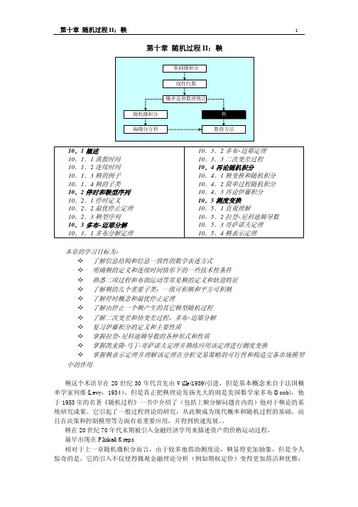
10.1.1 离散时间 简单的说,一个随机变量的时间序列没有表现出任何的趋势性(trend),就可以称之为鞅; 而如果它一直趋向上升,则称之为下鞅(submartingale);反之如果该过程总是在减少,则称 之为上鞅(supermartingale)。实际上鞅是一种用条件数学期望定义的随机运动形式,或者说 是具有某种可以用条件数学期望来进行特征描述的随机过程。 我们循序渐进地分成 4 个步骤来正式定义鞅: 1)首先,描述概率空间。存在一概率空间{Ω, F , P} ,要求σ-代数 F 是 P-完备的,即对 于任何 A ∈ F 且 P(A) = 0 ,对一切 N ⊂ A 都有 N ∈ F 成立2。接下来,
X :Ω→R 来描述信息结构。考虑这样一种的随机变量函数,它赋予一个分割中的同一子集下 的元素以相同的数值,我们称这种随机变量对于该种特定的分割是可测的。仍然使用前 面的二项树模型来具体说明这一点。有随机变量函数 x' ,它定义股票的价格在 0 时刻为 0,在 0 时刻以后则每经历一次上升就在原来的价格上加 1;如果下降就减去 1,图 10-1 中就标明这种情形。根据 x' 的定义有:
并且由于可以借助现代数值计算技术,它还提供了更为强大的运算能力,而这对于实际工 作又是至关重要的。
在本章中,我们首先在离散时间下,使用在概率基础一章中接触到的分割、条件数学 期望等概念来严格地给出鞅的定义。然后澄清一些性技术要求并给出连续时间鞅的概念。 介绍一些常见的鞅的例子。在讨论了鞅的两个重要子类之后,
F b 集合表示股票价格两次变动以后所有可能发生的情况,它仅仅说明了事物发展的 未来潜在可能性,它相当于位于二项树上的 0 点。在 0 时刻信息结构是最平凡的,即: F 0 = {∅, Ω}。而 F a 则刚好相反,它完全揭示出所有的世界状态,正是在最终的 2 时刻, 究竟哪种状态会发生已经成为了事实。 F c 则代表了一种中间状态,好比在 1 时刻,我 们知道如果状态 {uu,ud} 发生,即前进到 d[1] 点后, {dd} 或者 {ud} 之一必定会发生,到
高数下册知识点

高等数学下册(同济大学第七版)知识点高等数学下册知识点下册预备知识第八章 空间解析几何与向量代数(一) 向量及其线性运算1、 向量,向量相等,单位向量,零向量,向量平行、共线、共面;2、 线性运算:加减法、数乘;3、 空间直角坐标系:坐标轴、坐标面、卦限,向量的坐标分解式;4、 利用坐标做向量的运算:设),,(z y x a a a a = ,),,(z y x b b b b = , 则 ),,(z z y y x x b a b a b a b a ±±±=±, ),,(z y x a a a a λλλλ= ;5、 向量的模、方向角、投影:1) 向量的模:222z y x r ++= ;2) 两点间的距离公式:212212212)()()(z z y y x x B A -+-+-=3) 方向角:非零向量与三个坐标轴的正向的夹角γβα,,4) 方向余弦:rz r y r x ===γβαcos ,cos ,cos 1cos cos cos 222=++γβα5) 投影:ϕcos Pr a a j u =,其中ϕ为向量a 与u 的夹角。
(二) 数量积,向量积1、 数量积:θcos b a b a=⋅1)2a a a =⋅高等数学(下)知识点 2)⇔⊥b a 0=⋅b az z y y x x b a b a b a b a ++=⋅2、 向量积:b a c⨯= 大小:θsin b a ,方向:c b a ,,符合右手规则1)0=⨯a a 2)b a //⇔0=⨯b a z y x z y x b b b a a a k j i b a =⨯ 运算律:反交换律 b a a b⨯-=⨯(三) 曲面及其方程1、 曲面方程的概念:0),,(:=z y x f S2、 旋转曲面: yoz 面上曲线0),(:=z y f C ,绕y 轴旋转一周:0),(22=+±z x y f 绕z 轴旋转一周:0),(22=+±z y x f3、 柱面:0),(=y x F 表示母线平行于z 轴,准线为⎪⎩⎪⎨⎧==00),(z y x F 的柱面 4、 二次曲面1)椭圆锥面:22222zbyax=+2)椭球面:1222222=++czbyax旋转椭球面:1222222=++czayax3)单叶双曲面:1222222=-+czbyax4)双叶双曲面:1222222=--czbyax5)椭圆抛物面:zbyax=+22226)双曲抛物面(马鞍面):zbyax=-22227)椭圆柱面:12222=+byax8)双曲柱面:12222=-byax9)抛物柱面:ay x=2(四)空间曲线及其方程1、 一般方程:⎪⎩⎪⎨⎧==0),,(0),,(z y x G z y x F 2、 参数方程:⎪⎪⎩⎪⎪⎨⎧===)()()(t z z t y y t x x ,如螺旋线:⎪⎪⎩⎪⎪⎨⎧===btz t a y t a x sin cos 3、 空间曲线在坐标面上的投影⎪⎩⎪⎨⎧==0),,(0),,(z y x G z y x F ,消去z ,得到曲线在面xoy 上的投影⎪⎩⎪⎨⎧==00),(z y x H(五) 平面及其方程1、 点法式方程:0)()()(000=-+-+-z z C y y B x x A法向量:),,(C B A n = ,过点),,(000z y x2、 一般式方程:0=+++D Cz By Ax 截距式方程:1=++cz b y a x 3、 两平面的夹角:),,(1111C B A n = ,),,(2222C B A n = ,222222212121212121cos C B A C B A C C B B A A ++⋅++++=θ⇔∏⊥∏21 0212121=++C C B B A A⇔∏∏21// 212121C C B B A A ==4、 点),,(0000z y x P 到平面0=+++D Cz By Ax 的距离:222000C B A DCz By Ax d +++++=(六) 空间直线及其方程1、 一般式方程:⎪⎩⎪⎨⎧=+++=+++022221111D z C y B x A D z C y B x A 2、 对称式(点向式)方程:p z z n y y m x x 000-=-=-方向向量:),,(p n m s = ,过点),,(000z y x3、 参数式方程:⎪⎪⎩⎪⎪⎨⎧+=+=+=ptz z nt y y mt x x 000 4、 两直线的夹角:),,(1111p n m s = ,),,(2222p n m s = ,222222212121212121cos p n m p n m p p n n m m ++⋅++++=ϕ⇔⊥21L L 0212121=++p p n n m m⇔21//L L 212121p p n n m m ==5、 直线与平面的夹角:直线与它在平面上的投影的夹角,222222sin p n m C B A CpBn Am ++⋅++++=ϕ⇔∏//L 0=++Cp Bn Am⇔∏⊥L pC n B m A ==第九章 多元函数微分法及其应用(一) 基本概念(了解)1、 距离,邻域,内点,外点,边界点,聚点,开集,闭集,连通集,区域,闭区域,有界集,无界集。
基于多分辨率奇异谱熵和支持向量机的断路器机械故障诊断方法研究

但 其 训 练速 度 慢 、过 学 习 和 易 陷 入 局 部 极 小 值 点
等 问题 。支 持 向量 机 ( VM) 是 一 种 通 用 机 器 学 S
习方 法 ,对 于 小 样 本 、非 线 性 、 高 维 数 和 局 部 极
信 号 包 含 了 断 路 器 内 部 多 方 面 的 状 况 信 息 ,断 路 小 点 等 实 际 问题 能 比较 好 地 克 服 ’ 。 器运行状 态 异 常时 都会 在 振动 信 号 中有 所体 现 , 本 文 将 多 分 辨 率 奇 异 谱 分 析 与 支 持 向量 机 结
关 键词 :高压断路 器 ;多分辨 率奇异谱 熵;支持 向量机 ;故障诊断
中 图分 类 号 :T 6 M5 1 文献 标 识 码 :A
神 经 网络虽 然 具 有 较 强 的 学 习 和非 线 性 识 别 能 力 ,
0 引言
断 路 器 动 作 过 程 中 伴 随 强 烈 的 振 动 ,该 振 动
1 基 于 多 分 辨率 奇 熵是 基 于 信 号 的时 频 ,分 析 实
- 1、下载文档前请自行甄别文档内容的完整性,平台不提供额外的编辑、内容补充、找答案等附加服务。
- 2、"仅部分预览"的文档,不可在线预览部分如存在完整性等问题,可反馈申请退款(可完整预览的文档不适用该条件!)。
- 3、如文档侵犯您的权益,请联系客服反馈,我们会尽快为您处理(人工客服工作时间:9:00-18:30)。
多重分形奇异谱的几何特性I_经典Renyi定义法_周炜星Vol.26No.42000-08华东理工大学学报Journ al of East Chin a University of Science an d T echnology 基金项目:国家重点基础研究发展规划项目(G1999022103)E -mail:****************.cn收稿日期:1999-09-08作者简介:周炜星(1974-),男,浙江诸暨人,博士生,现从事湍流中非线性现象的理论和实验研究。
文章编号:1006-3080(2000)04-0385-05多重分形奇异谱的几何特性I .经典Renyi 定义法周炜星*, 王延杰, 于遵宏(华东理工大学洁净煤技术研究所,上海200237)摘要:研究了经典多重分形理论中广义维数和奇异谱的几何特性,通过严格的数学推导证明了广义维数D ~q 、质量指数S ~(q )、奇异性指数A ~(q )和奇异谱f ~(A ~(q ))的单调性和极限,并提出了判定合理奇异谱f ~(A ~(q ))的准则。
关键词:多重分形;奇异谱;广义维数;经典Renyi 定义法中图分类号:O4;O184文献标识码:AGeometrical Characteristics of Singularity Spectra of MultifractalsI .Classical Renyi DefinitionZH OU W ei -x ing *, W A N G Yan -j ie , YU Zun -hong(I nstitute of Clean Coal T echnology ECUS T ,Shanghai 200237,China )Abstract :It is w ell know n that multifractal theo ry is aneffective and w idely applied method to charac-terize a lot of nonlinear physical pheno mena in nature .In this paper ,the geometrical characteristics of sin-gularity spectra of multifractals defined via classical Reny i information are studied.The relev ant pr operties of the generalized dim ensio ns,scaling ex ponents,sing ularity str ength and singularity spectrum are derived rigo rously.It seems that the curve o f generalized dim ensions is sim ilar to that o f singularities w hen para-meter q tends to infinity .Especially ,we sho uld point o ut that singularity spectra cur ve lies in the first quadrant,w hose endpo ints are not necessary to be nought.An analy tical but simple pr ocedure to calculate the asym ptotic value at infinite is presented.It is found that different alg orithm s of first order derivative,and the com putation spacing as w ell ,lead to different multifractal spectrum .Therefore ,a criterion is sug-gested to determ ine the proper sing ular ity spectr um .T his is based on the fact that ,the curve of the m ulti-fractal spectrum is tangent to the diag onal of the first quadr ant,w hich implies that f ≤A for all q .Further-more,there is only one point o f intersection between tw o m ultifractal spectra arising from tw o different sy stems ,w hich is suppor ted by ex perimental and num er ical results .Key words :multifractal;sing ularity spectrum;generalized dimension;classical Reny i definition自从M andelbro t 在70年代提出分形概念以来,分形理论在物理、天文、地理、数学、生物、化学[1~7]、计算机[8]等科学领域得到了广泛的应用,并取得了大量富有新意的成果。
但是,随着理论研究和应用的深入,研究者们越来越清楚地意识到,对于大多数客观存在的分形物体而言,仅用一个分形维数并不能完全刻画其结构。
80年代初,Grassber ger 等系统地提出了多重分形理论,用广义维数和多重分形谱来描述分形客体,考虑了物理量在几何支集的385空间奇异性分布[9~11],因而在湍流、DLA、地震[12~13]等几乎所有涉及分形的领域迅速地取得了广泛应用。
通过计算机模拟或实验测定,可以得到广义分维和多重分形谱,但对其中不少结论存在着争议,因而有必要系统地研究广义分维和多重分形谱的几何特性,提出实际数值计算中对奇异谱的判定准则。
本文以多重分形理论为基础,重新定义并研究了4个连续函数D~q、S~(q)、A~(q)和f~(A~(q))的几何特性,提出了计算多重分形谱f(A)的判定准则。
1 用Reny i信息量定义多重分形的基本原理设F是d维分形空间(Fractal Space[8])上的分形集,一般地,我们可以用N个尺度为E i(i=1,2…N)的互不相交的d维微元C i将F覆盖,并在每个d维立方体C i上定义归一化概率测度P i。
命E= max{E i∶i=1,2…N},如果E足够小,那么可以认为P i在C i上的分布是均匀的,则可以定义奇异性标度指数A为P i~E A i(1)其中测度的不同区域有一A与之对应。
特别地,用N 个具有相等尺度E的互不相交的d维立方体覆盖分形集F,假设A在区间[A′,A′+d A′]上取某个值的次数为Q(A′)E-f(A′)d A′(2)其中,Q(A)表示奇异值A的密度,连续函数f(A)反映了A取值的次数。
为确定连续函数f(A),需要引入可测量的维数集合广义维数D q,Grassberg er、Hentschel和Pro-caccia等人将之定义为[9~10]D q=limE→01q-1lg V(q)lg E(3)其中V(q)=∑Ni=1P q i(4)是概率测度的q阶矩。
显然,D0是测度支集上的分形维数D f,D1=limq→1D q为信息维数R,D2是容量维数M。
将方程(1)和(2)代入(4),得到V(q)=∫E q A′Q(A′)E-f(A′)d A′(5)假定Q(A′)非零,由于E很小,故式(4)的积分在q A′-f(A′)取极小值时对V(q)贡献最大。
因而我们可用A(q)代替A′,其中A(q)满足极值条件dd A′[q A′-f(A′)]?A′=A(q)=0(6)d2d(A′)2[q A′-f(A′)]?A′=A(q)>0(7)于是f′(A(q))=q(8)f″(A(q))<0(9)定义函数S(q)为S(q)=q A-f(A)(10)则由式(3)得D q=S(q)q-1(11) 所以,如果知道f(A)和A值的谱,便可以求出广义维数D q。
同样,如果知道了广义维数D q,由式(8)和(10)可得奇异值A的计算公式A(q)=S′(q)(12)并由式(10)求出f(A)。
在实际应用中,只要测定归一化概率测度P i,就可以计算广义维数D q,从而得到多重分形的奇异性谱f(A)。
但是实验研究发现,计算时对分形集F 的划分、计算步长及计算方法选择不同,可能得到存在某种相关性但具有完全不同的几何特性的一族奇异谱f(A)。
2 多重分形的几何特性Hentschel和Procaccia首先较为系统地研究了奇怪吸引子的无穷广义维数集合D q在q>0时的性质[10],本文将他们的结果进行推广,考察了更为一般的情况。
设多重分形集处于无标度区,对于一E∈(0,1),N=[1/E]+1[1/E]<1/E[1/E][1/E]=1/E,任意给定测度P i∈(0,1),满足归一化条件∑Ni=1P i=1,记P max=maxi=1,2…N{P i},P min=mini=1,2…N{P i},-∞<q<+∞,[?]表示取整函数。
< bdsfid="138" p=""></q<+∞,[?]表示取整函数。
<>2.1 广义维数D~q的性质定理1 定义关于实数q的连续函数D~q=1q-1lg∑Ni=1P q ilg E(13)那么(1)D~′q≤0,当且仅当所有P i相等时“=”成立;(2)极限D~+∞和D~-∞都存在,并且386 华东理工大学学报第26卷D ~+∞>lim q →+∞D ~q =lg P max /lgE (14)D ~-∞>lim q →-∞D ~q =lg P min /lgE (15)证明(1)由推广的H lder 不等式[14~15]知,对于任意给出的正数列{a i ∶i =1,2…N }及实数-∞<+∞,有<=""<+∞,有<="" ∑N<+∞,有<="" i =1<+∞,有<="" (P<+∞,有<="" i<+∞,有<="" A s i<+∞,有<="" )<+∞,有<="" 1s<+∞,有<="" ≤<+∞,有<="" ∑N<+∞,有<="" i =1<+∞,有<="" (P<+∞,有<="" i<+∞,有<="" A t i<+∞,有<="" )<+∞,有<="" 1t<+∞,有<="" 当且仅当A i 全相等时取等号。