信号与系统双语课件chapter3.3
信号与系统第三章PPT课件
.
它们都是傅里叶级数收敛的充分条件。相当广泛的 信号都能满足Dirichlet条件,因而用傅里叶级数表 示周期信号具有相当的普遍适用性。
几个不满足Dirichlet条件的信号
.
三.Gibbs现象 满足 Dirichlet 条件的信号,其傅里叶级数是如
• “非周期信号都可以用正弦信号的加权积分来 表示”——傅里叶的第二个主要论点
.
傅立叶分析方法的历史
古巴比伦人 “三角函数和” 描述周期性过程、预测天体运
动
1748年 欧拉 振动弦的形状是振荡模的线性组合
1753年 D·伯努利 弦的实际运动可用标准振荡模的线性组合来表示
1759年 拉格朗日 不能用三角级数来表示具有间断点的函数
x[k]h[nk]
x[k]h[n k]
k
.
对时域的任何一个信号 x ( t ) 或者 x ( n ) ,若能将其
表示为下列形式: x(t) a 1 es1 t a 2 es2 t a 3 es3 t
由于 es1t H(s1)es1t
es2t H(s2)es2t
es3t H(s3)es3t
利用齐次性与可加性,有
k
例: y(t)x(t3) ❖ 系统输入为 x(t) ej2t
系统 H(s) ? y(t) ?
H(s) h(t)estdt
❖ 系统输入为 x(t)cos(4t)cos(7t)
系统 y(t) ?
.
*问题:究竟有多大范围的信号可以用复指数信号的 线性组合来表示?
.
3.3 连续时间周期信号的傅里叶级数表示
第k次谐波 e jk 0t 的周期为
信号与系统 奥本·海姆第三章课件
st
discrete time
z
n
z
n
e
st
h (t )
y (t )
h(n)
y (n)
Using Time domain analysis method,
y (t )
y[ n ]
e
s ( t )
h ( ) d e
st
h ( ) e
n
s
d H ( s )e
5
3、Lagrange criticized the use of trigonometric series to examine vibrating string in 1759.
4、Fourier claimed that any periodic signal could be represented by harmonically related sinusoids in 1807.
H (z)
k
h (n ) z
n
usefulness of decomposition in terms of eigenfunction
x(t ) ak e
k sk t
is important for the analysis of LTI systems . If :
y (t ) ak H ( sk )e
性质)
Chapter 3: Fourier Series Representation of Periodic Signals
2
3.0 Introduction(引言)
The basis for time domain (chapter 2) 1) Signal can be represented as combination of shifted impulses。 2) System is LTI。
《信号与系统》第三章习演示课件
k0 k 1
yt1 8 cos2t
3
Problem Solution
H j
2
1
3 0 3
图2
Chapter 3
Problem Solຫໍສະໝຸດ tion例 已知图1所示连续时间系统中输入信号 xt ,t2k k 两个子系统的频率响应 H1 和j H分2 别j如 图2和图3
所示。试求该系统的输出信号 y 。t
ak 0 k18
Chapter 3
Problem Solution
3.34 Consider a continuous-time LTI system hte4t Find the Fourier series representation of the output yt
for each of the following inputs :
sin 0t
c o s0 t L H j0 c o s 0 t H j0 s i n 0 t L H j0 s i n 0 t H j0
Chapter 3
Problem Solution
Consider an LTI system S with impulse response ht sint
(a)xttn n
(bx)t1ntn n
(c) xt is the periodic wave depicted in Figure P3.34
1/ 2 1 xt
-2 -1
0
1
2
t
Chapter 3
Problem Solution
例 研究图1所示的连续时间系统,其中 h1 t sin3tt, H1 j 和 H2 j的波形如图2所示。
信号与系统第三章课件

(n 0)
1 1 Fn An an 2 bn 2 2 2 bn n n arctg a ( n 0) n F0 a0 A0 (n 0)
f (t )
Fn
n T 1 2
Fn e jn 0t
f (t )e jn0t dt
n 1,2,
2 bn f (t ) sin n 0 tdt n 1,2, 《信号与系统》SIGNALS AND SYSTEMS T T
ZB
2 0 为基波频率,n0为谐波频率,an和bn为傅里叶系数, T
[]dt表示从任意起始点 开始,取一个周期 为积分区间。 T
f (t )
...
0
T 4 T 2
...
T
t
4. 奇谐函数: f (t ) f (t T ) ,则 只含奇次谐波。
2
f (t )
...
T 2
T
...
0
《信号与系统》SIGNALS AND SYSTEMS
T 2
t
ZB
3.1.2 指数型傅里叶级数
由欧拉公式
sin n0t 1 jn0t 1 e e jn0t , cosn0t e jn0t e jn0t 2j 2
3.3.1 周期信号的单边频谱和双边频谱
单边幅度频谱( n ~ n0 ) A 单边频谱 单边相位频谱( n ~ n0 ) 双边幅度频谱(Fn ~ n0 ) 双边频谱 双边相位频谱( n ~ n0 )
jn0t
抽样函数
sin x Sa ( x ) x
1. 偶函数
信号与系统目录(Signal and system directory)
信号与系统目录(Signal and system directory)Chapter 1 signals and systems1.1 INTRODUCTION1.2 signalContinuous signals and discrete signalsTwo. Periodic signals and aperiodic signalsThree, real signal and complex signalFour. Energy signal and power signalThe basic operation of 1.3 signalAddition and multiplicationTwo, inversion and TranslationThree, scale transformation (abscissa expansion)1.4 step function and impulse functionFirst, step function and impulse functionTwo. Definition of generalized function of impulse functionThree. The derivative and integral of the impulse functionFour. Properties of the impulse functionDescription of 1.5 systemFirst, the mathematical model of the systemTwo. The block diagram of the systemCharacteristics and analysis methods of 1.6 systemLinearTwo, time invarianceThree, causalityFour, stabilityOverview of five and LTI system analysis methodsExercise 1.32The second chapter is the time domain analysis of continuous systemsThe response of 2.1LTI continuous systemFirst, the classical solution of differential equationTwo, about 0- and 0+ valuesThree, zero input responseFour, zero state responseFive, full response2.2 impulse response and step responseImpulse responseTwo, step response2.3 convolution integralConvolution integralTwo. The convolution diagramThe properties of 2.4 convolution integralAlgebraic operations of convolutionTwo. Convolution of function and impulse function Three. Differential and integral of convolutionFour. Correlation functionExercise 2.34The third chapter is the time domain analysis of discretesystemsThe response of 3.1LTI discrete systemsDifference and difference equationsTwo. Classical solutions of difference equationsThree, zero input responseFour, zero state response3.2 unit sequence and unit sequence responseUnit sequence and unit step sequenceTwo, unit sequence response and step response3.3 convolution sumConvolution sumTwo. The diagram of convolution sumThree. The nature of convolution sum3.4 deconvolutionExercise 3.27The fourth chapter is Fourier transform and frequency domainanalysis of the systemThe 4.1 signal is decomposed into orthogonal functions Orthogonal function setTwo. The signal is decomposed into orthogonal functions 4.2 Fourier seriesDecomposition of periodic signalsTwo, Fourier series of odd even functionThree. Exponential form of Fu Liye seriesThe spectrum of 4.3 period signalFrequency spectrum of periodic signalTwo, the spectrum of periodic matrix pulseThree. The power of periodic signal4.4 the spectrum of aperiodic signalsFirst, Fu Liye transformTwo. Fourier transform of singular functionsProperties of 4.5 Fourier transformLinearTwo, parityThree, symmetryFour, scale transformationFive, time shift characteristicsSix, frequency shift characteristicsSeven. Convolution theoremEight, time domain differential and integral Nine, frequency domain differential and integral Ten. Correlation theorem4.6 energy spectrum and power spectrumEnergy spectrumTwo. Power spectrumFourier transform of 4.7 periodic signals Fourier transform of sine and cosine functionsTwo. Fourier transform of general periodic functionsThree 、 Fu Liye coefficient and Fu Liye transformFrequency domain analysis of 4.8 LTI systemFrequency responseTwo. Distortionless transmissionThree. The response of ideal low-pass filter4.9 sampling theoremSampling of signalsTwo. Time domain sampling theoremThree. Sampling theorem in frequency domainFourier analysis of 4.10 sequencesDiscrete Fourier series DFS of periodic sequencesTwo. Discrete time Fourier transform of non periodic sequences DTFT4.11 discrete Fu Liye and its propertiesDiscrete Fourier transform (DFT)Two. The properties of discrete Fourier transformExercise 4.60The fifth chapter is the S domain analysis of continuous systems 5.1 Laplasse transformFirst, from Fu Liye transform to Laplasse transformTwo. Convergence domainThree, (Dan Bian) Laplasse transformThe properties of 5.2 Laplasse transformLinearTwo, scale transformationThree, time shift characteristicsFour, complex translation characteristicsFive, time domain differential characteristicsSix, time domain integral characteristicsSeven. Convolution theoremEight, s domain differential and integralNine, initial value theorem and terminal value theorem5.3 Laplasse inverse transformationFirst, look-up table methodTwo, partial fraction expansion method5.4 complex frequency domain analysisFirst, the transformation solution of differential equation Two. System functionThree. The s block diagram of the systemFour 、 s domain model of circuitFive, Laplasse transform and Fu Liye transform5.5 bilateral Laplasse transformExercise 5.50The sixth chapter is the Z domain analysis of discrete systems 6.1 Z transformFirst, transform from Laplasse transform to Z transformTwo, z transformThree. Convergence domainProperties of 6.2 Z transformLinearTwo. Displacement characteristicsThree, Z domain scale transformFour. Convolution theoremFive, Z domain differentiationSix, Z domain integralSeven, K domain inversionEight, part sumNine, initial value theorem and terminal value theorem 6.3 inverse Z transformFirst, power series expansion methodTwo, partial fraction expansion method6.4 Z domain analysisThe Z domain solution of difference equationTwo. System functionThree. The Z block diagram of the systemFour 、 the relation between s domain and Z domainFive. Seeking the frequency response of discrete system by means of DTFTExercise 6.50The seventh chapter system function7.1 system functions and system characteristicsFirst, zeros and poles of the system functionTwo. System function and time domain responseThree. System function and frequency domain responseCausality and stability of 7.2 systemsFirst, the causality of the systemTwo, the stability of the system7.3 information flow graphSignal flow graphTwo, Mason formulaStructure of 7.4 systemFirst, direct implementationTwo. Implementation of cascade and parallel connectionExercise 7.39The eighth chapter is the analysis of the state variables of the system8.1 state variables and state equationsConcepts of state and state variablesTwo. State equation and output equationEstablishment of state equation for 8.2 continuous systemFirst, the equation is directly established by the circuit diagramTwo. The equation of state is established by the input-output equationEstablishment and Simulation of state equations for 8.3discrete systemsFirst, the equation of state is established by the input-output equationTwo. The system simulation is made by the state equationSolution of state equation of 8.4 continuous systemFirst, the Laplasse transform method is used to solve the equation of stateTwo, the system function matrix H (z) and the stability of the systemThree. Solving state equation by time domain methodSolution of state equation for 8.5 discrete systemsFirst, the time domain method is used to solve the state equations of discrete systemsTwo. Solving the state equation of discrete system by Z transformThree, the system function matrix H (z) and the stability of the systemControllability and observability of 8.6 systemsFirst, the linear transformation of state vectorTwo, the controllability and observability of the systemExercise 8.32Appendix a convolution integral tableAppendix two convolution and tableAppendix three Fourier coefficients table of commonly used periodic signalsAppendix four Fourier transform tables of commonly used signalsAppendix five Laplasse inverse exchange tableAppendix six sequence of the Z transform table。
信号与系统课件(英文)讲解
x[n] Balance in bank y[n]
(sytem
x(t)
t1 y(t)
t2
1 Signal and System
1.6.4 Stability
x[n]
Discrete-time y[n]
System
SISO system
MIMO system?
1 Signal and System
1.5.1 Simple Example of systems
Example 1.8:
RC Circuit in Figure 1.1 : Vc(t) Vs(t)
Memoryless system: It’s output is dependent only on the input at the same time. Features: No capacitor, no conductor, no delayer.
Examples of memoryless system: y(t) = C x(t) or y[n] = C x[n]
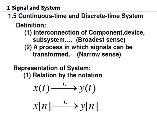
Representation of System: (1) Relation by the notation
x(t) L y(t)
x[n] L y[n]
1 Signal and System
(2) Pictorial Representation
x(t) Continous-time
System
信号与系统SignalsandSystemsppt课件
0.5
0.4
0.3
0.2
0.1
0
0
1
2
3
4
5
6
7
8
9
10
1
0.9
0.8
0.7
0.6
0.5
0.4
0.3
0.2
0.1
0
0
1
2
3
4
5
6
7
8
9
10
一、基本信号的MATLAB表示
% rectpuls
t=0:0.001:4; T=1; ft=rectpuls(t-2*T,T); plot(t,ft) axis([0,4,-0.5,1.5])
rand
产生(0,1)均匀分布随机数矩阵
randn 产生正态分布随机数矩阵
四、数组
2. 数组的运算
数组和一个标量相加或相乘 例 y=x-1 z=3*x
2个数组的对应元素相乘除 .* ./ 例 z=x.*y
确定数组大小的函数 size(A) 返回值数组A的行数和列数(二维) length(B) 确定数组B的元素个数(一维)
0.3
0.2
0.1
function [f,k]=impseq(k0,k1,k2) 0
-50 -40 -30 -20 -10
0
10 20 30 40 50
%产生 f[k]=delta(k-k0);k1<=k<=k2
k=[k1:k2];f=[(k-k0)==0];
k0=0;k1=-50;k2=50;
[f,k]=impseq(k0,k1,k2);
已知三角波f(t),用MATLAB画出的f(2t)和f(2-2t) 波形
信号与系统PPT全套课件
T T
T
f (t ) dt
f (t ) dt
2
2
(1.1-1)
1 P lim T 2T
T
T
( 1.1-2 )
上两式中,被积函数都是f ( t )的绝对值平方,所以信号能量 E 和信号功率P 都是非负实数。 若信号f ( t )的能量0 < E < , 此时P = 0,则称此信号 为能量有限信号,简称能量信号(energy signal)。 若信号f ( t )的功率0 < P < , 此时E = ,则称此信 号为功率有限信号,简称功率信号(power signal)。 信号f ( t )可以是一个既非功率信号,又非能量信号, 如单位斜坡信号就是一个例子。但一个信号不可能同时既是 功率信号,又是能量信号。
1.3 系统的数学模型及其分类
1.3.1 系统的概念 什么是系统( system )?广义地说,系统是由若干相互作用 和相互依赖的事物组合而成的具有特定功能的整体。例如, 通信系统、自动控制系统、计算机网络系统、电力系统、水 利灌溉系统等。通常将施加于系统的作用称为系统的输入激 励;而将要求系统完成的功能称为系统的输出响应。 1.3.2 系统的数学模型 分析一个实际系统,首先要对实际系统建立数学模型,在数 学模型的基础上,再根据系统的初始状态和输入激励,运用 数学方法求其解答,最后又回到实际系统,对结果作出物理 解释,并赋予物理意义。所谓系统的模型是指系统物理特性 的抽象,以数学表达式或具有理想特性的符号图形来表征系 统特性。
2.连续信号和离散信号 按照函数时间取值的连续性划分,确定信号可分为连续时 间信号和离散时间信号,简称连续信号和离散信号。 连续信号( continuous signal)是指在所讨论的时间内,对 任意时刻值除若干个不连续点外都有定义的信号,通常用f ( t ) 表示。 离散信号(discrete signal)是指只在某些不连续规定的时刻 有定义,而在其它时刻没有定义的信号。通常用 f(tk) 或 f(kT) [简写 f(k )] 表示,如图1.1-2所示。图中信号 f (tk) 只在t k = -2, -1, 0, 1, 2, 3,…等离散时刻才给出函数值。
信号与系统ppt课件
a 0 呈单调指数上升。
精品课件
a 0 呈单调指数下降。 a 0 x(t) C 是常数。
2. 周期性复指数信号:
a j0,不失一般性取
C 1 x (t) ej 0 t c o s0 tjsin0 t
• 连续时间情况下:
E lT im T Tx(t)2d t x(t)2dt
•离散时间情况下:
N
E N l i m nNx(n)2n x(n)2
精品课件
在无限区间内的平均功率可定义为:
x(t) P
lim1 T2T
T T
2
dt
PN l i m 2N 11nN Nx(n)2
精品课件
1.2 自变量变换
究确知信号。
精品课件
连续时间信号的例子:
精品课件
离散时间信号的例子:
精品课件
连续时间信号在离散 时刻点上的样本可以构成一个 离散时间信号。
精品课件
二. 信号的能量与功率:
连续时间信号在 [ t1 , t 2 ] 区间的能量定义 为:
E t2 x(t) 2 dt t1
连续时间信号在 [ t1 , t 2 ]
率定义为:
区间的平均功
P 1 t2 x(t)2 dt
t2 t1 t1
精品课件
离散时间信号在 [ n1 , n 2 ]
的能量定义为n2
E
x(n) 2
n n1
区间
离散时间信号在 [ n1 , n 2 ] 平均功率为
P 1
n2 x(n)2
n2 n11nn1
精品课件
区间的
在无限区间上也可以定义信号的总 能量:
•给定信号和系统求变换后的 信号。
信号与系统课件(英文)
or
{ak }
x(t ) ak
are called Fourier Series coefficients or spectral coefficients of .
FS
x(t )
3 Fourier Series Representation of Periodic Signals 1 (t ) Note:About orthogonality
e
e
j 0t
,e
j 0t
: Fundamental components
j 20t
,e
j 20t
: Second harmonic components
e
jN0t
,e
jN 0t : Nth harmonic components
So, arbitrary periodic signal can be represented as ( Fourier series )
e
jk 0T1
]
3 Fourier Series Representation of Periodic Signals
sin k0T1 sin k0T1 ak 2 k0T k
(3.44)
0T 2
1 a0 T
2T1 dt T T1
T1
So,Fourier Series Representation of
Discrete time LTI system:
x[n] ak zk
k 1
N
n
y[n] ak H ( zk ) zk
k 1
N
n
H ( z)
3 Fourier Series Representation of Periodic Signals Example 3.1
- 1、下载文档前请自行甄别文档内容的完整性,平台不提供额外的编辑、内容补充、找答案等附加服务。
- 2、"仅部分预览"的文档,不可在线预览部分如存在完整性等问题,可反馈申请退款(可完整预览的文档不适用该条件!)。
- 3、如文档侵犯您的权益,请联系客服反馈,我们会尽快为您处理(人工客服工作时间:9:00-18:30)。
Since the product x(t)y(t) is also periodic with period T, we can expand it in a Fourier series with Fourier series coefficients hk expressed in terms of those for x(t) and y(t). The result is
The Dirichlet conditions are as follow: Condition 1. over any period, x(t) must be absolutely integrable, that is x(t ) dt
T
Condition 2. In any finite interval of time, x(t) is of bounded variation; that is, there are no more than a finite number of maxima and minima during any single period of the signal. Condition 3. In any finite interval of time, there are only a finite number of discontinuities. If a signal satisfy the Dirichlet conditions, it can be represented by Fourier series.
FS x(t ) ak
to signify the pairing of the periodic signal with its Fourier series coefficients. That means the Fourier series coefficients of x(t) are {ak}
3.5.2 Time shifting
If
FS x(t ) ak
Then
FS x(t t0 ) e jk0t0 ak e jk (2 / T )t0 ak
One consequence of this property is that, when a periodic signal is shifted in time, the magnitudes of its Fourier series coefficients remain unaltered. That is,
x(t ) y(t ) hk
FS
l
a b
l k l
3.5.6 Conjugation and conjugate symmetry
If
FS x(t ) ak
FS x (t ) a k
x (t ) is the complex conjugation of the periodic signal x(t).
a k is the complex conjugation of the periodic signal a-k.
3.5.7 Parseval’s relation for continuoustime periodic signals
The parseval’s relation :the total average power in the a periodic signal equals the sum of the average power in all of its harmonic components
FS x(t ) ak FS y(t ) bk
Then the Fourier series coefficients ck of the linear combination of x(t) and y(t), z(t) =Ax(t)+By(t), are given by the same linear combination of the Fourier series coefficients for ak and bk.
★ An consequence of this property is that if x(t) is even, then its Fourier series coefficients are also even. Similarly , if x(t) is odd, the its Fourier series coefficients are also odd.
For a signal
x[n] e
j0n
It is a periodic signal with fundamental frequency 0 2 / N and fundamental period N .
Associated with this signal is the set of harmonically related complex exponentials
ak bk
3.5.3 Time reversal
If
FS x(t ) ak FS x(t ) ak
Then
Time reversal applied to a continuous-time signal results in a time reversal of the corresponding sequence of Fourier series coefficients.
3.5.1 Linearity
Let x(t) and y(t) denote two periodic signals with period T and which have Fourier series coefficients denote by ak and bk, respectively.
3.5 Properties of continuous-time Fourier series
Fourier series representations possess a number of important properties that are useful for developing conceptual insights into such representations, and they can also help to reduce the complexity of the evaluation of Fourier series of many signals. Throughout the following discussion of the selected properties, we will use the notation
2 1 x(t ) dt ak T T k 2
3.6 Fourier series representation of dicrete-time periodic signals
3.6.1 Linear combination of harmonically related complex exponential
1 1 jk0t ak x(t )e dt T T T
T
x(t )e jk ( 2 / T )t dt
We denote integration over any interval of length T by
T
3.4 Convergence of the Fourier series
review
If a signal x(t) has a Fourier series representation in the form of
x(t )
k
ak e
jk0t
k
jk ( 2 / T ) t a e k
Then the coefficients are given by
FS z(t ) Ax(t ) By(t ) ck Aak Bbk
The period of z(t) is also T.
Representation of the periodic signal z(t) as a weighted sum of periodic square waves: z(t) = (3/2)x(t) + 1/2y(t). (a) z(t). (b) x(t). (c) y(t).
k [n] e jk n e jk (2 / N ) n , k 0,1,2,....
0
There are only N distinct signals in the this set. why? From section 1.3.3, we know a fact that discrete-time complex exponentials which differ in frequency by a multiple of 2πare identical. So :
k [n] e jk n e jk (2 / N ) n , k 0,1,2,....
0
Each of these signals has a fundamental frequency that is a multiple of0 and therefore, each is periodic with period T.
k [n] k rN [n]
That is ,when k is changed by any integer multiple of N, the identical sequence is generated.
Now we wish to consider the representation of more generally periodic sequences in terms of linear combinations of the sequences k [n] ,such a linear combination has the form