傅立叶光学基本原理
2-1衍射和傅里叶光学基础详解

2.1.1 标准形式的一维非初等函数
(1) 矩形函数
又称为门函数,表示为
rect(x)
rect x 或 x
1
1 rect(x) 1/ 2
0
x 1/ 2 x 1/ 2 x 1/ 2
x -1/2 O 1/2
rect( x)dx 1
曲线下面积为1,表示矩形光源、狭缝或矩形孔的透射率
(2)sinc 函数
与某函数相乘使其极性翻转
sgn(x)
1 x
0 -1
(5)阶跃函数
• 定义:
1 step(x) 1/ 2
0
x0 x0 x0
step(x )
1 x
0
表示刀口或直边衍射物体或开关信号等
(6)圆柱函数
1 circ(r) 1/ 2
0
r 1 r 1 r 1
Circ (r)
1
y
x
O
1
circ(
x2 a
y2
22
1、直角坐标系中的二维非初等函数
(1)二维矩形函数,定义式为:
1
rect(x, y) rect(x)rect( y) 1/ 2
0
————可分离变量函数
| x | 1/ 2and | y | 1/ 2 | x || y | 1/ 2
| x | 1/ 2and | y | 1/ 2
rect(x, y)
1
在光学问题中,常用来描述一个均匀 照明方形小孔的振幅透射系数。
二维矩形函数的一般表达式为:
1
1
2
rect( x x0 , y y0 ) rect( x x0 )rect( y y0 )
图11
ab
傅里叶变换光学系统

傅里叶变换光学系统傅里叶变换光学系统,简称FT光学系统,是一种通过光学方法对物体进行分析的技术。
其基本原理是利用傅里叶变换的思想,将物体在空间域的信息转换为频域的信息,然后通过相同的方式将频域信息还原为空间域信息。
一、傅里叶变换的基本原理傅里叶变换是一种将函数从时域转换到频域的技术。
其基本原理是将一个函数按照不同频率分解成一系列正弦波的和。
具体来说,傅里叶变换可以分为以下几个步骤:1. 对原函数在时间域上进行分段,使其转化为一系列长度为Δt 的小区间。
2. 对每一个小区间的函数值进行离散化处理,生成离散的数据序列。
3. 对离散的数据序列进行傅里叶变换,求出在频域上的频率分量。
4. 通过反傅里叶变换,将在频率域的信息还原为在时间域上的信息。
二、傅里叶变换在光学系统中的应用在光学系统中,傅里叶变换可以将一个物体的透射率函数转换为空间域和频域的关系。
通过加入透镜、像差校正等光学器件,可以实现将频域信息转换为对应的光学信号,进而生成一个光学图像。
这种光学图像可以对物体进行解析,便于对物体形状、大小、结构等信息进行研究。
FT光学系统广泛应用于生物医药、材料科学、光学工程等领域中。
三、傅里叶变换光学系统的优点与不足优点:1. 精度高:通过光学技术,可以获取高精度的物体信息,尤其是对于那些复杂的结构物体。
2. 兼容性好:FT光学系统可以与其他光学测量仪器、成像系统等进行互相配合,丰富了光学分析工具的功能。
3. 速度快:由于光子的速度极快,FT光学系统的成像速度也可以达到很高的水平。
不足:1. 设备成本高:由于FT光学系统需要使用高质量、高精度的光学仪器,因而设备成本较高。
2. 实验难度大:FT光学系统需要经过实验测试,对于初学者来说,实验难度比较大。
3. 约束条件多:FT光学系统对光源、光路、光学器件等条件的约束较多,安装过程比较繁琐。
总之,傅里叶变换光学系统在解析复杂物体、研究物体结构等方面有很大优势,并得到了广泛应用。
傅立叶光学基本原理

傅立叶光学基本原理实验目的:在4f 系统中,观察不同的衍射物通过两个凸透镜后的傅立叶变换,计算栅格常数实验原理:傅立叶变换,惠更斯原理,多缝衍射,阿贝成像原理该实验使用当中,在进行相干光学处理时,采用了如下图所示的双透镜系统(即4f 系统)。
这时输入图像(物)被置于透镜L1的前焦面,若透镜足够大,在L1的后焦面上即得到图像准确的傅立叶变换(频谱)。
并且,因为输入图像在L1的前焦面,需要利用透镜L2使像形成在有限远处。
在4f 系统中,L1的后焦面正好是L2的前焦面,因此系统的像面位于L2的后焦面,并且像面的复振幅分布是图像频谱准确的傅立叶变换。
物面L1 频谱面 L2 像面从几何光学看,4f 系统是两个透镜成共焦组合且放大倍数为1的成像系统。
在单色平面波照明下(相干照明),当输入图像置于透镜L1的前焦面时,在L1的后焦面上得到图像函数E *(x,y )准确的傅立叶变换:E *(x,y )=⎰⎰∞+∞-+-∞+∞-⨯dadb e b a E f y x A b f y a f x B B B )(2),(),,(λλπ其中,x,y 是L1后焦面(频谱面)的坐标。
由于L1的后焦面与L2的前焦面重合,所以在L2的后焦面又得到频谱函数E *(x,y )的傅立叶变换,略去常数因子:⨯=)ˆ,ˆ,ˆ(ˆ)ˆ,ˆ(ˆB f y x A y x E ⎰⎰∞+∞-+-∞+∞-dadb e b a E b f y a f x B B )ˆˆ(2),(λλπ通过两次傅立叶变换,像函数与物函数成正比,只是自变量改变符号,这意味着输出图像与输入图像相同,只是变成了一个倒像。
第一次傅立叶变换把物面光场的空间分布变为频谱面上的空间频率分布,第二次傅立叶变换又将其还原到空间分布。
相干光学信息处理在频谱面上进行,通过在频谱面上加入各种空间滤波器可以达到改变频谱而达到处理图像信息的目的。
通过在物面处加上光栅,通过光的多缝干涉,使得不同空间频率的图像信息叠加在一起(空间频率是在空间呈现周期性分布的几何图形或物理量在某个方向上单位长度内重复的次数)。
傅里叶光学的实验报告(3篇)

第1篇一、实验目的1. 深入理解傅里叶光学的基本原理和概念。
2. 通过实验验证傅里叶变换在光学系统中的应用。
3. 掌握光学信息处理的基本方法,如空间滤波和图像重建。
4. 理解透镜的成像过程及其与傅里叶变换的关系。
二、实验原理傅里叶光学是利用傅里叶变换来描述和分析光学系统的一种方法。
根据傅里叶变换原理,任何光场都可以分解为一系列不同频率的平面波。
透镜可以将这些平面波聚焦成一个点,从而实现成像。
本实验主要涉及以下原理:1. 傅里叶变换:将空间域中的函数转换为频域中的函数。
2. 光学系统:利用透镜实现傅里叶变换。
3. 空间滤波:在频域中去除不需要的频率成分。
4. 图像重建:根据傅里叶变换的结果恢复原始图像。
三、实验仪器1. 光具座2. 氦氖激光器3. 白色像屏4. 一维、二维光栅5. 傅里叶透镜6. 小透镜四、实验内容1. 测量小透镜的焦距实验步骤:(1)打开氦氖激光器,调整光路使激光束成为平行光。
(2)将小透镜放置在光具座上,调节光屏的位置,观察光斑的会聚情况。
(3)当屏上亮斑达到最小时,即屏处于小透镜的焦点位置,测量出此时屏与小透镜的距离,即为小透镜的焦距。
2. 利用夫琅和费衍射测光栅的光栅常数实验步骤:(1)调整光路,使激光束通过光栅后形成衍射图样。
(2)测量衍射图样的间距,根据dsinθ = kλ 的关系式,计算出光栅常数 d。
3. 傅里叶变换光学系统实验实验步骤:(1)将光栅放置在光具座上,调整光路使激光束通过光栅。
(2)在光栅后放置傅里叶透镜,将光栅的频谱图像投影到屏幕上。
(3)在傅里叶透镜后放置小透镜,将频谱图像聚焦成一个点。
(4)观察频谱图像的变化,分析透镜的成像过程。
4. 空间滤波实验实验步骤:(1)将光栅放置在光具座上,调整光路使激光束通过光栅。
(2)在傅里叶透镜后放置空间滤波器,选择不同的滤波器进行实验。
(3)观察滤波后的频谱图像,分析滤波器对图像的影响。
五、实验结果与分析1. 通过测量小透镜的焦距,验证了透镜的成像原理。
光学傅里叶变换原理

光学傅里叶变换原理傅里叶变换是一种数学工具,用于将一个函数( 或信号)从时间 或空间)域转换到频率域。
在光学中,傅里叶变换也具有重要的应用,尤其是在描述光波传播、光学系统和图像处理等方面。
傅里叶变换原理涉及到以下重要概念和原则:1.(傅里叶级数:傅里叶级数指的是将周期性函数分解为一系列正弦和余弦函数的和的过程。
它表明任何周期性函数都可以表示为不同频率的正弦和余弦函数的叠加。
2.(连续傅里叶变换 Continuous(Fourier(Transform):对于连续信号,傅里叶变换将信号从时域转换到频域。
它描述了信号在频率空间中的频谱特性,展示了信号由哪些频率分量组成。
3.(离散傅里叶变换 Discrete(Fourier(Transform):对于离散数据集合,比如数字图像或采样信号,离散傅里叶变换用于将这些离散数据从时域转换到频域。
它在数字信号处理和图像处理中得到广泛应用,用于分析和处理频率特性。
4.(光学中的应用:在光学中,傅里叶变换可以描述光的传播和衍射现象。
例如,傅里叶光学理论表明,光学系统(如透镜、光栅等)可以看作是对光波进行空间域的傅里叶变换。
这种理论有助于理解光的传播特性,并在光学系统设计和成像技术中发挥重要作用。
5.(变换原理:傅里叶变换原理表明,任何一个信号都可以通过傅里叶变换分解成一系列不同频率的正弦和余弦函数。
这种变换可以帮助我们理解信号的频率成分,并对信号进行处理、滤波或合成。
总的来说,傅里叶变换原理提供了一种从时域到频域的转换方法,在光学中,它被广泛应用于光波传播、光学系统设计和图像处理等领域,为我们理解和处理光学现象提供了重要的工具。
第6章 傅里叶光学基础 (1)
= α F {g} + β F {h} ,即两个(或多个)函数之加权和 A. 线性定理。 F {α g + β h}
的傅里叶变换就是各自的傅里叶变换的加权和。 B.相似性定理。若 F{g ( x, y )} = G ( f X , fY ) ,则 F{g (ax, by )} = 1 f X fY , G ab a b (6-7)
5
对非周期函数也可以作傅里叶分析,只是其频率取值不再是离散的,而是连 续的。 (1) 二维傅里叶变换 非 周 期 函 数 g ( x, y ) 在 整 个 无 限 xy 平 面 上 满 足 狄 里 赫 利 条 件 , 而 且
∫∫
∞
−∞
g ( x, y ) dxdy 存在,则有
= g ( x, y ) 其中
6
即空域 ( x, y ) 中坐标的“伸展” ,导致频域 ( f X , fY ) 中坐标的压缩,加上频域的 总体幅度的一个变化。 C.相移定理。若 F{g ( x, y )} = G ( f X , fY ) ,则 F {g ( x − = a, y − b)} G ( f X , fY ) exp[ − j 2π ( f X a + fY b)] 即原函数在空域的平移,将使其频谱在频域产生线性相移。 D. 帕塞瓦尔定理。若 F{g ( x, y )} = G ( f X , fY ) ,则 (6-8)
−bn an
图 6-1 画出了锯齿波及它的振幅频谱图形。由图看出,周期函数的频谱具有 分立的结构。
f ( x)
cn
O
x
(a )
O
f1 f 2 f 3 f 4 (b)
fn
图 6-1 锯齿波及其频谱 将一个系统的输入函数 g ( x) 展开成傅里叶级数,在频率域中分析各谐波的 变化,最后综合出系统的输出函数,这种处理方法称作频谱分析方法。频谱分析 方法在光学中的应用, 为认识复杂的光学现象及进行光信息处理提供了全新的思 路和手段。 6.1.4 傅里叶变换
光学4f系统的傅里叶变换原理
光学4f系统的傅里叶变换原理
光学4f系统是一种常见的光学传递系统,由两个透镜组成,分别称为前透镜和后透镜,它们之间的距离为f。
该系统可以实现对输入光场的傅里叶变换。
傅里叶变换原理是指输入光场通过光学4f系统后,可以得到输出光场的傅里叶变换。
傅里叶变换是一种将时域信号转换为频域信号的数学变换方法,可以将一个信号分解成一系列的频率成分。
在光学4f系统中,输入光场首先经过前透镜,前透镜将输入光场进行傅里叶变换,将其分解成一系列的平面波。
这些平面波经过后透镜后,再次叠加在一起,形成输出光场。
输出光场可以通过适当选择前透镜和后透镜的焦距以及它们之间的距离f,来实现对输入光场的傅里叶变换。
具体来说,如果前透镜的焦距为f1,后透镜的焦距为f2,则前透镜和后透镜之间的距离为f=f1+f2。
根据傅里叶变换的性质,输入光场经过前透镜后,可以表示为前透镜的传递函数H1与输入光场的乘积。
同样地,输出光场可以表示为后透镜的传递函数H2与前透镜的传递函数H1与输入光场的乘积。
因此,输出光场可以表示为H2H1与输入光场的乘积。
通过选择合适的传递函数H1和H2,可以实现对输入光场的傅里叶变换。
常见
的选择是使H1和H2为透镜的传递函数,即H1和H2都为复振幅调制函数。
这样,输出光场可以表示为输入光场的傅里叶变换。
总之,光学4f系统的傅里叶变换原理是通过选择适当的透镜传递函数,使得输入光场经过前透镜和后透镜后,可以得到输出光场的傅里叶变换。
这一原理在光学信号处理和图像处理中有广泛的应用。
第1章 傅里叶光学基础
(21)
(8) 矩 (moment) g(x,y)的(k,l g(x,y)的(k,l )阶矩定义为 M k, l = ∫∫∞- ∞ g(x,y)xk yl dxdy 将逆变换表达式( 代入上式, 将逆变换表达式(2)代入上式,得到
M k, l=∫∫∞-∞G(u,v)dudv∫∫∞-∞xkylexp[i2π(ux+vy)]dxdy G(u,v)du [i2π x+v
傅里叶-贝塞尔变换 傅里叶 贝塞尔变换 设函数g(r,θ) = g(r) 具有圆对称, 具有圆对称, 函数 θ 傅里叶-贝塞尔变换为 傅里叶 贝塞尔变换为 G(ρ) = B {g(r)} ρ = 2π ∫∞org(r)Jo(2πρr)dr g(r)J π r)dr π 其中 Jo 为第一类零阶贝塞尔函数 傅里叶-贝塞尔逆变换为 傅里叶 贝塞尔逆变换为 g(r) = B-1 {G(ρ)} ρ = 2π ∫∞o ρ G(ρ)Jo(2πρr)dρ π ρ J π r)dρ
第一章
傅里叶光学基础
第一章 傅里叶光学基础
1.1 二维傅里叶分析 1.2 空间带宽积和测不准关系式 1.3 平面波的角谱和角谱的衍射 1.4 透镜系统的傅里叶变换性质
1.1 二维傅里叶分析
1.1.1 定义及存在条件 傅里叶变换可表为 复变函数器 g(x,y) 的傅里叶变换可表为 G(u,v) = F {g(x,y)} = ∫∫∞- ∞g(x,y)exp[-i2π(ux+vy)]dxdy g(x,y)exp[x+vy)]dxdy (1) 为变换函数或像函数 称g(x,y)为原函数,G(u,v)为变换函数或像函数。 为原函数, 为变换函数或像函数。 (1)式的逆变换为 式的逆变换 式的逆变换为 g(x,y) = F -1{G(u,v) } = ∫∫∞- ∞G(u,v)exp[i2π(ux+vy)]dudv (2) exp[i2 x+vy)]du
傅立叶光学基本原理-2f和4f系统1 (2)
Pb06206250 李小龙实验二傅立叶光学基本原理-2f和4f系统实验目的观测和了解2f系统中一个透镜对物平面的光场的傅立叶变换作用,计算光栅的栅格常数。
观测和了解4f系统中两个透镜对物平面的光场的傅立叶变换作用及光学滤波,测量小孔直径。
实验元件HeNe激光,平面镜,透镜,f=+100mm ,白屏,光栅1,光栅,衍射物1,衍射物2,物镜(objective),20x,支架,尺子,实验步骤下文括号中的数字表示的坐标仅适用于开始阶段的粗调。
――如图1摆放器件。
――初期的调整,不需要E20x扩束系统(1,6)和透镜L0(1,3)。
――使用M1(1,8)和M2(1,1)调整光路时,要让光线沿平台的x=1和y=1的直线走。
――放置E20x和透镜L0(F=+150mm)在光路中,调整器件的位置以保证从透镜发出的光是平行光线,即随距离增大,光点不会发散。
用尺子在透镜L0后0.5m范围内不同距离处测量光点的直径。
检验其平行度,应保证不同距离处的圆形光斑的直径基本保持不变。
――摆放另外的光学元件。
其中P1为物平面,屏幕SC放在透镜L1(F=+100mm)的后焦距处,即构成2f系统。
图1 2f系统a)实验的第一步观察平面波(光斑),此时物平面没有放置衍射物体。
依据理论,在透镜L1后的傅立叶面SC应该出现的一个光点。
也称焦点。
b)将可调狭峰在物平面P1上,调整高度和截面的方位,使光点通过狭峰。
在屏幕上可以看到狭峰的傅立叶变换,即典型的单峰衍射图样(与理论比较)。
c)将光栅1(diffraction grating)放在P1,透镜L1后的傅立叶面SC上即为衍射图(the slit separation canbe made using the separation of the diffraction maxima in the Fourier planes SC behind the lens L1)。
计算该光栅的光栅常数。
光学第六篇傅里叶变换光学简介
复杂波场: 分解为一系列平面波或球面波成分
波的类型和特性 波前相因子
波前相因子
方向角的余角
线性相因子
系数(cosx,cosy)或 (sin1,sin2)与平面 波的传播方向一一对应。
U2 U1
ik x2 y2
e 2fBiblioteka 凹透镜和凸透镜的情况相同,
只是焦距一个为负,一个为正。
相位型
例题:求薄透镜傍轴成像公式:
在傍轴条件下:U1 ( x,
y)
ik x2 y2
A1e 2s
ik x2 y2
透镜函数:tL (x, y) e 2 f
s
s’
ik x2 y2
ik x2 y2
U2 (x, y) tL (x, y)U1(x, y) e 2 f
二维 tP ( x, y) eik (n1() 1x+2 y)
例题:推导棱镜傍轴成像公式:
傍轴条件:
ik x2 y2
s
U1(x, y) A1e 2s
ik x2 y2 ik (n1) x
U2 (x, y) tP (x, y) U1(x, y) A1e 2s
(n1)s 2 x(n1)s 2 y2
第六章 傅里叶变换光学简介
第六章 傅里叶变换光学简介
1、衍射系统 波前变换 2、相位衍射元件 3、波前相因子分析法 4、余弦光栅的衍射场 5、傅里叶变换 6、超精细结构的衍射 隐失波 7、阿贝成像原理与空间滤波 8、光学信息处理列举 9、泽尼克的相衬法
惠更斯-菲涅耳原理 光波衍射
菲涅耳衍射 夫琅禾费衍射
二维波前 决定 三维波场
二维波前 决定 三维波场
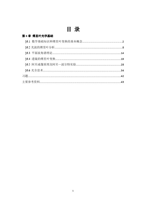
Double-helix Point Spread Function (DH-PSF) DH-PSF transfer function obtained from the iterative obtimization procedure, and its GL modal plane decomposition, which forms a cloud around the GL modal plane line. The DH-PSF transfer function does not have any amplitude component, and consequently is not absorptive.
- 1、下载文档前请自行甄别文档内容的完整性,平台不提供额外的编辑、内容补充、找答案等附加服务。
- 2、"仅部分预览"的文档,不可在线预览部分如存在完整性等问题,可反馈申请退款(可完整预览的文档不适用该条件!)。
- 3、如文档侵犯您的权益,请联系客服反馈,我们会尽快为您处理(人工客服工作时间:9:00-18:30)。
实验二傅立叶光学基本原理-2f和4f系统实验目的观测和了解2f系统中一个透镜对物平面的光场的傅立叶变换作用,计算光栅的栅格常数。
观测和了解4f系统中两个透镜对物平面的光场的傅立叶变换作用及光学滤波,测量小孔直径。
实验元件HeNe激光,平面镜,透镜,f=+100mm ,白屏,光栅1,光栅,衍射物1,衍射物2,物镜(objective),20x,支架,尺子,实验步骤下文括号中的数字表示的坐标仅适用于开始阶段的粗调。
――如图1摆放器件。
――初期的调整,不需要E20x扩束系统(1,6)和透镜L0(1,3)。
――使用M1(1,8)和M2(1,1)调整光路时,要让光线沿平台的x=1和y=1的直线走。
――放置E20x和透镜L0(F=+150mm)在光路中,调整器件的位置以保证从透镜发出的光是平行光线,即随距离增大,光点不会发散。
用尺子在透镜L0后0.5m范围内不同距离处测量光点的直径。
检验其平行度,应保证不同距离处的圆形光斑的直径基本保持不变。
――摆放另外的光学元件。
其中P1为物平面,屏幕SC放在透镜L1(F=+100mm)的后焦距处,即构成2f系统。
图1 2f系统a)实验的第一步观察平面波(光斑),此时物平面没有放置衍射物体。
依据理论,在透镜L1后的傅立叶面SC应该出现的一个光点。
也称焦点。
b)将可调狭峰在物平面P1上,调整高度和截面的方位,使光点通过狭峰。
在屏幕上可以看到狭峰的傅立叶变换,即典型的单峰衍射图样(与理论比较)。
c)将光栅1(diffraction grating)放在P1,透镜L1后的傅立叶面SC上即为衍射图(the slit separation can be madeusing the separation of the diffraction maxima in the Fourier planes SC behind the lens L1)。
计算该光栅的光栅常数。
将2f系统扩展为4f系统将提供的支架P2、透镜L2(f=+100mm)和白屏SC分别放置在距透镜L1一倍、二倍和三倍的焦距处,此时即构成4f系统。
(如右图)不带滤波器时的衍射图象1,将带有箭头的衍射物2放在P1,调整其位置,使得光照在图形的箭头处,记录下在屏上观测到的反置图形,并予理论解释;调整图象的位置,将其旋转90°,重复上述步骤。
2, 将箭头的图片换成国王的图片(衍射物3),让光束照亮脸部的轮廓,此时在屏上的图象是什么样的? 3, 将光栅2安装在P1,观测在P2、SC 的位置处的图象,(在SC 时,可将屏绕轴旋转(接近平行与光的传播方向,能否在屏上观测到光栅图象)? 滤波后的图象1, 将光栅2安装在P1,在P2放置带小孔的圆盘(直径1~2mm 的小孔),让中间的衍射最大通过。
观测小孔的直径渐小时,对SC 上光栅图象的影响。
当小孔直径小到某一值时,光栅像应基本消失。
2, 保持光路不变,将国王像(衍射物3)和光栅2(4lines/mm )的图片一起装在P1,在屏上能够观测到的合成图象和去掉小孔圆盘的图象相比有什么区别?3, 将激光直接照射到该小孔上,由其在墙上的衍射斑,计算出小孔的直径,该尺寸与光栅2的4lines/mm 的物理条件的关系如何?应用傅立叶变换的知识解释上述现象。
实验原理The Fourier transform plays a major role in the natural sciences . In the majority of cases , one deals with Fourier transforms in a time range ; they supply us with the spectral composition of a time signal . This concept can be extend - ed in two aspects :1 . In our case a spatial signal and not a temporal signal is transformed .2 . A two- dimensional transform is performed . From this , the following is obtained :[]dxdye y x E v v y x E v v E y v x v i y x y x y x ⎰⎰+∞∞-+∞∞-+-=ℑ=)(2,).()(),(),(~πWhere vxandvy: spatial frequencies . 标量衍射理论(scalar diffraction theory )In Fig . 2 we observe a plane wave which is diffracted in one plane . For this wave in the xy plane directly behind the planeZ = 0 with the following transmission distribution),(y x τ:),(),(),(y x E y x y x E e ∙=τwhere),(y x E e : electric field distribution of the incident wave.The 图 2further expansion can be described by the assumption that a spherical wave emanates from each point ( x , y , 0 ) behind the diffracting structure ( Huygens , principle ) . This leads to Kirchhoff ’s diffraction integral :dxdyr n r e y x E i z y x E ikr ),cos(),(1),,(⎰⎰∞+∞-∞+∞-=''λ (2)W ithλ= spherical wave length ; n= normal vector of the plane ( x , y ) ;k = wave number λπ/2Equation ( 2 ) corresponds to an accumulation of spherical waves , where the factor λi 1 is a phase and amplitudefactor and),cos(r n, a directional factor which results from the Maxwell field equations .The Fresnel approximation ( observations in a remote radiation field ) considers only rays which occupy a small angle to the optical axis ( 2 axis ) , i.e .zy x 〈〈, andzy x 〈〈'',. In this case , the directional factor can be neglectedand the 1/r dependence becomes : l/r =1/z . In the exponential function , this cannot be performed as easily since even small changes in r result in large phase changes . To achieve this , the roots in2222222)()(1)()(z y y z x x z z y y x x r -'+-'+∙=+-'+-'=are expanded into a series and one obtains :()()zy y z x x z r 2222-'+-'+=This results in the Fresnel approximation of the diffraction integral()()()()()dxdy e y x E i e z y x E y y x x z ikikz 222,,,-'+-'∞+∞-∞+∞-⎰⎰=''λ (3)For long distances from the diffracting plane with concurrent finite expansion of the diffracting structure , one obtains the FRAUNHOFER APPROXIMAT1ON :()()()dxdyey x E z y x C z y x E z z y x i ⎪⎪⎭⎫ ⎝⎛'+'-∞+∞-∞+∞-⎰⎰∙''=''λλπ2,,,,,(4)with()()22,,y x z i ikz ez i e z y x C '+'∙=''λπλwith the spatial frequencies as new coordinates : 图 3zx x λυ'=;zy y λυ'=Consequently the field distribution in the plane of observation ( x ' , y ' , z ) is shown by the following :()()()[]()()y x y x y x E y x E z z z C z y x E νννννλνλ,~,,,,,,=ℑ=''The electric field distribution in the plane (x ’,y ’) for z = const is thus established by a Fourier transform of the field strength disiribution in the diffracting plane after multiplication with a quadratic phase factorexp()()()22y x z i +π. The spatial frequencies are proportional to the corresponding diffraotion angles ( see Fig .3 ) , where :λλλν∂≈∂='=tan z x x ; λβλλν≈∂='=tan z y yThrough the making of a photographic recording or through observation of the diffraction image with one eye , the intensity formation disappears due to the phase information of the light in the plane (x ’,y ’z ). As a consequence , only the intensity distribution ( this corresponds to the power spectrum ) can be observed . As a consequence of the phase factor C , ( Equation6 ) drops out of the operation . Therefore , the following results :()()[]()222,,1,yx y x y x E z I ννλννℑ=一个透镜的傅立叶变换A biconvex lens exactly performs a two-dimensional Fourier transform from the front to the rear focal plane if the diffracting structure (entry field strength distribution ) lies in the front focal plane ( see Fig . 4 ) . In this process , the coordinates νand u correspond to the anglesβandαwith the following correlations :Bx f u z x λλαλν=='=; Byf uz y λλβλν=='=(8) This means that the lens projects the image of the remote radiation field in the rear focal plane :()()dxdyey x E f u A u E y f x f u B B B⎪⎪⎭⎫ ⎝⎛+-∞+∞-∞+∞-⎰⎰∙=λυλπνν2,,,),(~(9)The phase factor A becomes independent of u and v ,if the entry field distribution is positioned exactly in the front focal p lane . Thus , the complex amplitude spectrum results :()ν,~u E ~()[]()ν,,u y x E ℑAgain the power spectrum is recorded or observed :()()2,~,ννu E u I =~()[]2,y x E ℑ (10)It , too , is independent of the phase factor A and thus becomes independent of the position of the diffraction structure in the front focal plane . Additionally , equation ( 8 ) shows thatthe larger the图 4 focal length of the lens is , the more extensive the diffraction image in the (u,v )plane is .傅立叶谱的实例 a) 平面波A plane wave which propagates itself in the direction of the optical axis ( z axis ) ( Fig . 5 ) 15 distinguished in the object plane –( x , y ) plane- by a constant amplitude . Thus , the following results for the Fourier transform :()0,E y x E = (11)and()[]()()()y x yx i E dxdy eE y x E y x νδνδννπ∙==ℑ+-+∞∞-+∞∞-⎰⎰020,This is a point on the focal plane at (vx,vy )=(0,0) which shifts at slanted incidence by an angle αto the optical axison the rear focal plane(see Fig . 5 ) withλανsin =x ·图 5(b )有限宽度的无限长狭缝If the diffracting structure is an infinite slit which is transilluminated by a plane wave , this slit is mathematicallydescribed by a reotangular function " rect " perpendicular to the slit direction and having the same width a :(){210,a x for otherwiseEa x rect y x E 〈=⎪⎭⎫⎝⎛=In the rear focal plane the following spectrum then results :()[]()()()()()x y xx y a a yx i a c a E a E dxdy eE y x E yx ννδπννπνδννπsin sin ,002220∙=∙==ℑ⎰⎰∞+∞-+-+- (12)W ith the definition of the Slit function "sinc " :()()x x x c ∙∙=ππsin sinfor infinitely long extension of the slit , one obtains no extension in the slit direction in the spectrum . This changes for a finite length of the slit . The zero points of the " sinc " function are located at …-2/a,-1/a,1/a,2/a …(see Fig . 6 ) .图 6(c) 栅格A grid is a composite diffracting structure . It consists of a periodic sequence ( to be represented by a so-called comb function " comb " ) of individual identical slit functions " SinC " .The grid consists of M slits having a width a and a slit separation d ( > a ) in the x direction . As a result , the field strength distribution in the front focal plane can be represented as follows :()⎪⎭⎫⎝⎛*⎥⎦⎤⎢⎣⎡∙-=⎪⎭⎫ ⎝⎛∙-=∑∑==a x rect d m x E a d m a x rect E y x E M m Mm 1010(,δ where the Fourier transform of a convolution product (E1*E2)is given by :()()[]()()[]()[]()y x y x y x y x E y x E v y x E E ννννν,),(,,,,2121ℑ∙ℑ=*ℑUsing the calculation rules for Fourier transforms , the following spectrum results in the rear focal plane of the lens . :[]()()()()()()()x x M id x y Mm dv mi xx y d d M e a c a E e a E E x x νπνπννδπννπνδνπ∙∙∙∙∙∙=∙∙=ℑ+-=⋅-∑sin sin sin sin 10120 (13)As a consequence of the intensity formation , the phase factor cancels out :()()()()()x x x y y x d d M a c a E v I νπνπννδν∙∙∙=222220sin sin sin , (14)In Fig . 7 , a grid with its corresponding spectrum ( and the corresponding intensity distributions ) is presented . One sees from the spectrum that the envelope curve is formed by the spectrum of the individual slit which has a width a . The finer structure is produced by the periodicity , which is determined by the grid constant Md .图 7Coherent optical filtrationBy intervening in the Fourier spectrum,optical filtration can be performed; this can result in image improvement, etc . The appropriate operation for making the original image visible is again the inverse Fourier transform . Howeve it cannot be used here due to diffraction. The Fourier transform is again used; this leads to the 4f set- up ( see figure 3) Using the lst lens(L1), the spectrum with the appropriate spatial frequencies is generated in the Fourier plane from the original diffraction structure.In this plane,the spectrum can be altered by fading out specific spatial frequency fraction. A modifiec spectrum is created;it is again Fourier transformed by the 2nd lens(L2).If the spectrum is not altered,one obtains the original image in the inverse direction in the image plane (right focal plane of the 2nd lens,see also partial experiment(a) with the arrow diaphragm).This follows from the calculation of the twofold Fourier transformation:The simplest applications for optical fitration are the high and low-pass filtration .Low-pass raster eliminationIn the experiment,the photographic slide was provided with a grid by superimposing grid lines on it in one direction .The scanning theory states that a non-raster image(in this case :Emperor Maximilian) can be exactly reconstructed if the image is band-limited in its spectrum,i.e if it only contains spatial frequencies in the Fourier plane up to an upper limitingfrequencies.The raster image can be described mathematically as follows:This describes the grid lines and the non-raster image.The slit separation of the grid is b.The Fourier spectrum B(vx,vy) of the entire image becomes the following with the convolution law:Where G(vx,vy) is the Fourier transformation of the non-raster image. In addition we made use of the fact that the Fourier transformation of an comb function is also a comb function. This means that the Fourier spectrum is again a grid which is formed by the reiteration of the spectrum of the non-raster image. Each grid point with its immediate surrounding contains the total information of the non-raster image g(x,y).It is important, that the distance of the grid points in the Fourier plane is far enough, that the spectrum of the non-rastered picture (the slide) don’t overlap. However, only in this cases is it possible to filter out a single image point with a pinhole diaphragm. Fig,4(d) shows a situation, where the individual spectrums overlap too much, so that a filtering cannot be successful. This spatial frequency filtration can be considered as multiplication of the spectrum by an aperture function A(vx,vy)(pinhole diaphragm in the Fourier spectrum).In this case, an appropriate measuring dimension would be a diameter of ~1/b. Therefore, we obtain。