The Practice of Approximated Consistency for Knapsack Constraints

合集下载

Approximating and Intersecting Surfaces from Points

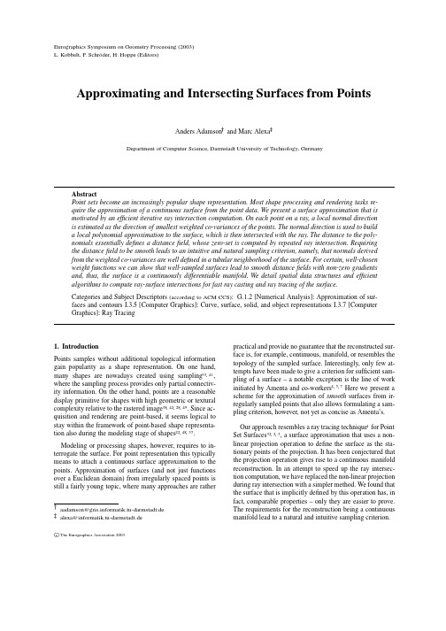
Eurographics Symposium on Geometry Processing(2003)L.Kobbelt,P.Schröder,H.Hoppe(Editors)Approximating and Intersecting Surfaces from PointsAnders Adamson and Marc AlexaDepartment of Computer Science,Darmstadt University of Technology,Germany AbstractPoint sets become an increasingly popular shape representation.Most shape processing and rendering tasks re-quire the approximation of a continuous surface from the point data.We present a surface approximation that is motivated by an efﬁcient iterative ray intersection computation.On each point on a ray,a local normal direction is estimated as the direction of smallest weighted co-variances of the points.The normal direction is used to builda local polynomial approximation to the surface,which is then intersected with the ray.The distance to the poly-nomials essentially deﬁnes a distanceﬁeld,whose zero-set is computed by repeated ray intersection.Requiring the distanceﬁeld to be smooth leads to an intuitive and natural sampling criterion,namely,that normals derived from the weighted co-variances are well deﬁned in a tubular neighborhood of the surface.For certain,well-chosen weight functions we can show that well-sampled surfaces lead to smooth distanceﬁelds with non-zero gradients and,thus,the surface is a continuously differentiable manifold.We detail spatial data structures and efﬁcient algorithms to compute ray-surface intersections for fast ray casting and ray tracing of the surface.Categories and Subject Descriptors(according to ACM CCS):G.1.2[Numerical Analysis]:Approximation of sur-faces and contours I.3.5[Computer Graphics]:Curve,surface,solid,and object representations I.3.7[Computer Graphics]:Ray Tracing1.IntroductionPoints samples without additional topological information gain popularity as a shape representation.On one hand, many shapes are nowadays created using sampling3341, where the sampling process provides only partial connectiv-ity information.On the other hand,points are a reasonable display primitive for shapes with high geometric or textural complexity relative to the rastered image38422849.Since ac-quisition and rendering are point-based,it seems logical to stay within the framework of point-based shape representa-tion also during the modeling stage of shapes224837. Modeling or processing shapes,however,requires to in-terrogate the surface.For point representation this typically means to attach a continuous surface approximation to the points.Approximation of surfaces(and not just functions over a Euclidean domain)from irregularly spaced points is still a fairly young topic,where many approaches are rather aadamson@rmatik.tu-darmstadt.dealexa@informatik.tu-darmstadt.de practical and provide no guarantee that the reconstructed sur-face is,for example,continuous,manifold,or resembles the topology of the sampled surface.Interestingly,only few at-tempts have been made to give a criterion for sufﬁcient sam-pling of a surface–a notable exception is the line of work initiated by Amenta and co-workers457Here we present a scheme for the approximation of smooth surfaces from ir-regularly sampled points that also allows formulating a sam-pling criterion,however,not yet as concise as Amenta’s. Our approach resembles a ray tracing technique1for Point Set Surfaces3223,a surface approximation that uses a non-linear projection operation to deﬁne the surface as the sta-tionary points of the projection.It has been conjectured that the projection operation gives rise to a continuous manifold reconstruction.In an attempt to speed up the ray intersec-tion computation,we have replaced the non-linear projection during ray intersection with a simpler method.We found that the surface that is implicitly deﬁned by this operation has,in fact,comparable properties–only they are easier to prove. The requirements for the reconstruction being a continuous manifold lead to a natural and intuitive sampling criterion.c The Eurographics Association2003.After establishing some context by brieﬂy discussing re-lated work(Section2),weﬁrst provide the theory using a slightly less general version of our surface deﬁnition(Sec-tion3)and then explain the iterative procedure(Section4) and spatial data structures(Section5).2.Related WorkWe concentrate on work that is directly related to our ap-proach,namely,the approximation of a surface from point samples and interrogating this surface by means of fast ray-surface intersections.Most approximation techniques deﬁne the surface implic-itly,either by deﬁning a scalar function of space or by certain constructive means.An interesting line of approximation algorithms deﬁne the surface as a subgraph of the Delaunay complex of the points1217.Many algorithms follow this spirit and differ mostly in how they identify triangles that belong to the sur-face.Crust457uses vertices of the V oronoi diagram as an approximation to the medial axis.The Delaunay triangula-tion including these vertices connects points on the surface either to the medial axis or to natural neighbors,which al-lows identifying surface triangles.The connection to the me-dial axis leads naturally to a minimal sampling density that is linear in the proximity of the surface to the medial axis. Sufﬁcient sampling guarantees a reconstruction of the origi-nal topology.Cocone61415has similar guarantees but elim-inates the step of adding V oronoi vertices to the point set. This makes the Delaunay-complex signiﬁcantly smaller and, thus,the reconstruction faster.Still,constructing the Delau-nay complex of millions of points is costly and some algo-rithm rather use local triangulations of the points1120 Hoppe et al.25deﬁnes an implicit function that is interest-ingly in a sense dual to Delaunay-type reconstruction:For each point a normal direction is estimated from neighboring points and all normals are oriented consistently.The signed distance to the surface is deﬁned as the normal component of the distance to the closest point.Thus,the surface consists of planes through the points bounded by the V oronoi cells of the points.In many practical cases one has multiple point samples for the same region.A way to consolidate this information is to build a distance function in a volumetric grid by properly weighting the points1347.Deﬁning the surface as a set of planar pieces results in C0 approximations.To achieve smoother approximations one could either build a smooth surface over the triangulation24 orﬁt smoother functions.A global and smooth interpolant for scattered data can be constructed using radial basis func-tions(RBF).For surface approximation an implicit function is computed using extra points away from the surface4345. The computation traditionally involves the solution of a large linear system,however,is nowadays tackled using com-pactly supported functions46,mulitpole expansions8109, thinning18192616,or hierachical clustering2736.Another approch is toﬁt globally smooth functions locally21,or to perform purely localﬁts3930and blend these local surface approximations together35.The moving least squares(MLS)31approximation takes this approach to the extreme by building a localﬁt for every point on the ing MLS allows deﬁning a projection operation that deﬁnes the surface implicitly as its stationary points32. The projection operation could be used for resampling the surface23.Our surface deﬁnition results from simplifying a ray intersection procedure1for this type of surface.For modeling and rendering a surface has to be interro-gated.While for rendering one could use the the existing points38422849,modeling typically requires operations such as ray-surface intersection,for example,to specify points on the surface by clicking.For a variety of deformation and CSG operations the MLS projection operator could be used37.Computing ray-surface intersections for an implicit sur-face is conceptually simple:The ray is substituted in the im-plicit surface deﬁputing the intersection is,thus, equivalent toﬁnding a root of a function in one unknown. To speed up the intersection computation one should ex-ploit properties of the implicit function.A common way is to compute a(local)Lipschitz constant,which yields a con-servative step width2923.Another approach is to use interval analysis34.Schauﬂer and Jensen deﬁne a ray-surface intersection for point sets directly,without an intermediate surface deﬁnition44.They collect points within a cylinder around the ray and compute a weighted average surface location.This is very fast,however,the geometry resulting from ray surface intersection depends on the particular rays used for intersect-ing the surface.3.Foundations–Simple Surface Deﬁnition andSampling CriterionWe assume that a set of points implicitly deﬁnes a smooth manifold surface.More speciﬁcally,let points p i3i 1N,be sampled from a surface S(possibly with ameasurement noise).The general idea of our surface def-inition is inspired by MLS approximation–the surface is approximated by building local polynomial approximations everywhere in space and a point s in space belongs to the surface if its local polynomial approximation contains s.For reasons of clarity weﬁrst describe a slightly simpliﬁed ver-sion of the deﬁnition.We feel this makes the connection to the sampling criterion and the resulting properties easier to establish.The more general surface deﬁnition is given later together with an algorithm that computes ray surface inter-sections.c The Eurographics Association2003.The main tools for the deﬁnition of the surface are weighted averages and weighted co-variances of the points in a tubular neighborhood around the surface.A weight func-tionθ:speciﬁes the inﬂuence of a point p i using the euclidean distance,i.e.θi xθp i x.Weight func-tions are assumed to be smooth,positive,and monotonicallydeacreasing(have positiveﬁrst derivative).The weighted average of points at a location s in space isa s ∑N1i0θi s p i∑N1i0θi s(1)and the weighted co-variance at s in direction n describes how well a plane n s x0ﬁts the weighted points:σ2n s ∑N1i0θi s n s p i2∑N1i0θi s(2)Letσs be the vector of weighted co-variances along the directions of the canonical baseσs σ100sσ010sσ001s(3)then the major axes(i.e.directions of smallest and largest weighted co-variance at a point s)are accesible as the eigen-vectors of the bilinear formΣsσsσs T(4) where an eigenvalue is the co-variance along the direction of the associated eigenvector.Our computation and deﬁnition of the surface mainly de-pends on local frames,which are built from locally estimated normals.Deﬁnition1The normal direction n x x3(or normal for short)is deﬁned as a direction of smallest weighted co-variance,i.e.min nσ2n x.If n is unique the normal is well-deﬁned.It is clear that the normal in x is given as the eigenvector of the co-variance matrixΣx corresponding to the smallest eigenvector.The normal is well-deﬁned exactly ifΣx has an eigenvalue that is strictly smaller than all other eigenval-ues.We deﬁne the surface implicitly based on normal direc-tions and weighted averages.The implicit function f:3 describes the distance of a point x to the weighted average a x projected along the normal direction n x:f x n x a x x(5)As always,the approximated surface is deﬁned as the zero-set of the implicit function,i.e.x:f x0(6) We know from differential geometry that is a smoothFigure1:The surface is deﬁned implicitly as the zero set of a function f x.In each point x a local normal direction n x is estimated as the direction of minimal weighted co-variance.The implicit function f x describes the distance of a weighted average a x of the points along normal direc-tion.differentiable manifold if f is a smooth function with non-zero gradient at least in anε-tubular neighborhood around the zero-set.Requiring f to be smooth leads to a surprisingly simple and natural sampling criterion:Deﬁnition2A surface S is well-sampled with points p i and approximated by if the normals are well-deﬁned in-side a tubular neighborhood around.We will show that this condition is sufﬁcient for f being smooth for points x inside the tubular neighborhood:First note that f is a smooth function in a and n.If all weight func-tions are smooth,the weighted average a and the weighted co-variance matrix are smooth functions in x.Furthermore, eigenvalues are smooth functions in the matrix coefﬁcients and eigenvectors are the solution of a linear system in the eigenvalues and the matrix.Since the normal direction is de-ﬁned as the eigenvector corresponding to the smallest eigen-value,n x is smooth in x as long as one eigenvector is always associated with the smallest eigenvalue.This has to be the case if the smallest eigenvalue is always strictly smaller than all other eigenvalues,i.e.,if all normals are well-deﬁned.The topology of the approximated surface depends on the particular choice of weight functionsθi.It is clear that certainθi could lead to non-manifold approximations and that even if is manifold it’s not necessarily homoemorphic to S.On the other hand,weights could be so chosen that is manifold and,with further restrictions,resembles the topology of S.To give an intuition for this,weﬁrst consider an inﬁnites-imal ball B around s.Inside the ball,weights are constant and so are a x and n x.Thus,for this region f describes a plane and if this plane passes the ball the approximation ofc The Eurographics Association2003.inside B is a disk.If,furthermore,the gradient of f inside such ball is non-zero,is manifold.We show in the Ap-pendix that using Gaussians as weight functions is sufﬁcient for non-zero gradient at f x0.For homeomorphic reconstruction the support of the weights should be so chosen that they separate differentsheets of the surface(note that sufﬁcient sampling is a pre-requisite for differentiation of sheets).As Gaussians have in-iﬁnite support we have no practical means to construct theo-retically correct weights yet,however,in practice Gaussians with approriate radius perform quite nicely(as is demon-strated in Section6).4.Ray-surface intersectionsThe surface deﬁnition given in the previous section implies a technique to efﬁciently compute ray-surface intersections. The idea is to evaluate function f,as it provides a rough approximation of the distanceﬁeld to for f x0.For ﬁxed n and a Equation5describes the planarﬁtl x n s a s x(7)to S with respect to the location s(depicted by the dashed line in Figure1).The smaller the distance f s is,the better S is approximated in q,which is the projection of x onto l along n.If f s0q s is a point on the surface.The approximation l is used to converge to S along a ray r, using an iterative scheme similar to the ray tracing approach for MLS-surfaces1.Once an approximation is determined, the equation r r o s t d is inserted in l x,and solving l r0provides t d for the intersection of ray and planarsurface approximation.The series of intersections r i ap-proaches the surface.In theory,once r i is close enough to the surface,the series f r i f r i1f r i2is strictly descreasing and an increase could be used to bail out off the iteration and start over.In practice,however,we have to accomodate imperfect weighting and use more tolerant it-eration conditions:We require that the closest point q on the approximated surface is close to the current position on the ray r i that has been used to compute q as well as close to the next intersection r i1of the ray and the plane l0through q.Speciﬁcally,a region of trust T around q has to contain r i and r i1.If not,the iteration is terminated and no ray surface intrsection in the proximity of r0could be reported.How to obtain an initial point r0is discussed later in Sec-tion5.The region T depends on the weighting-function for n x and a x,which affects the size of features in.How to make suitable choices for the weighting-function and T is also addressed in Section5.The procedure sketched above is easily generalized by taking the following point of view:In each point on r a local coordinate system is created using the approximation of a normal direction.In this coordinate system a weighted least square constant approximation to the surface is computedHFigure2:In an intermediate approximation of the ray sur-face intersection r i a local coordinate system H is estab-lished using the direction of minimal weighted co-variance as the normal n(the weighted average is a constant least squares approxima-tion).This local approximation is intersected with the ray and the procedure is repeated.In this setting it seems quite natural to use higher order least squares approximations to the surface in the local coordinate system in an attempt to increase the approximation order of the scheme.In retro-spect,we have used constant polynomials for the analysis because this allows explicitly solving the linear system that determines the polynomial.The following three steps are iterated until the sequence r0r1r2converges to the ray-surface intersection or the procedure is terminated,focussing on the next region to be examined:1.Support plane:The normal of a support plane H in r i isdetermined by minimizing the weighted distances of the points p j to H.The weights are computed from the dis-tances of the p j to r i using a smooth,positive,monotone decreasing functionθ(e.g.a gaussianθd e d2h2).This weighted least squares problem is solved by minimizingN∑j1n p j r i2θp j r i(8)The minimization of equation8can be rewritten in bilin-ear formminn1n T B n(9) where B b kl is the matrix of weighted co-variancesb lkN∑j1θj p jkr ikp jlr ilThe minimization problem in equation9is solved byc The Eurographics Association2003.HFigure3:The local coordinate system H is used to com-pute a local bivariate polynomial approximation to.This approximation is intersecte with r to yield the next approxi-mation to the ray surface intersection r i1.computing the eigenvector of B with the smallest eigen-value.The resulting H is approximately parallel to the Surface in the area around its nearest approach to r i.2.Polynomial approximation:The support plane in r i isused to compute a local bivariate polynomial approxima-tion a i of.To determine the coefﬁcients of a i,again a weighted least squares problem is solved by minimizing the equationN∑j1a i x j y j f j2θp j r i(10)where x j y j is the projection of p j onto H in normal direction and f j n p j r i is the height of p j overH.Equation10can be minimized by calculating its gra-dient over the unknown coefﬁcients of the polynomial.This leads to a system of linear equations,which is solved using standard numerical methods.The resulting polyno-mial is a local approximation of the surface.If r i is sufﬁciently close to,a i is expected be a good approxi-mation to around r i and the intersection r i1of the ray with a i could be used to converge to.3.Intersection:If the ray intersects a i,this point r i1serves as the starting point for the next iteration.If the ray misses a i the iteration is terminated.Only ray-polynomial intersections within T are considered.An intersection is detected,when the constant part c of a i is zero.In prac-tice a c being smaller then aεsufﬁces to accept r i(or the ray-intersection with a i)as an adequate ray-surface intersection.5.Spatial data structuresIn this Section we describe how to represent a tubular neigh-borhood around the surface.This neighborhood is needed to make sure that the intersection procedure described earlier starts from a suitable point r0.Moreover,using simple primi-tives for the representation of the neighborhood signiﬁcantly speeds-up ray surface intersection.In practice,the size of a tubular neighborhood around the surface that contains only well-deﬁned normals is unknown a-priori.Our best choice is to construct a spatial region that has a certain maximum dis-tance to the point set as we expect the distance of the points to the reconstructed surface to be bounded.Speciﬁcally,we construct a set of balls B i of radiusρi around the points p i.If the surface is contained in the union of the balls the balls are a bounding volume of that is easy to test for intersection.If a ray intersects,it also in-tersects at least one ball containing the intersection.Thus,an intersected ball indicates a potential ray surface intersection. The radius h has to be chosen,to ensure thatN∑i0B i(11)Unfortunately,is unknown a priori.The only a-priori knowledge are the points p i,which are expected to be very close to the surface.Therefore,we choose conservative radiiρi,so that each B i encloses the k-nearest neighbors of p i.In practice,we use k 6.The intersection of a ray with the set of balls can be com-puted efﬁciently.To quickly determine a subset of poten-tially intersected balls,the balls are arranged within an oc-tree(see Figure4),which is traversed along the ray using a parametric algorithm40.The current octree-voxel provides the candidate balls to be tested against the ray.Intersected balls are sorted along the ray to ensure that theﬁrst ray sur-face intersection is computed.Each ray ball intersection is handled as follows:The cen-ter p i of B i is used as initial point s for the construction of a local coordinate system and polynomial approximation a i. Using p i for this approximation instead of the ray ball in-tersection has two reasons:First,p i is expected to be close to and should provide a reasonable approximation of the surface around p i.Second,the coordinate system and poly-nomial approximation within B i are independent of the ray and can be stored for intersection with the next ray that in-tersects B i.Intersecting the ray with a i yields r0.Figure4 illustrates this idea.Then the procedure detailed in Section4is applied using B i as the region of trust T.Thus,if the ray intersects the polynomial approximation inside B i,the step is repeated un-til the desired accuracy is reached;otherwise no ray surface intersection is found within B i and the next intersected ball along the ray is inspected.Sometimes it is not important to determine theﬁrst in-tersection along a ray but only if there is any intersection with the object.A prominent example for rendering algo-rithms are shadow rays in ray tracing.Once a shadow-ray isc The Eurographics Association2003.Figure4:The spatial data structres used to represent a tubular neighborhood around is constructed as union of balls around the points.This region has the property that it contains all points with a certain maximum distance to the points and represents a best guess to the tubular neighbor-hood as points are expected to be close to the surface.For reducing the number of ray sphere intersections an octree is used.obstructed by an opaque object,it is not necessary to deter-mine at what position the rayﬁrst hits that object.Such a ray can be simply discarded from the illumination computa-tions.This speciﬁc ray intersection query can be optimized byﬁnding an intersection as quickly as possible anywhere on the ray.As spheres intersected close to their center are more likely to contain an intersection with the surface,they are sorted according to the distance d i from the ray to the center c i.The following equation determines the priorityγi of a sphere considering different radiiρi.γiρi d iρi(12)6.Applications&ResultsWe have used the ray surface intersection algorithm to com-pute renderings by means of ray tracing.In practice,we use Gaussian weights,i.e.θi x exp x p i2h2.The global parameter h allows specifying the locality of the ing smaller values for h results in a more lo-cal approximation,larger values could be used to smooth out small variations in the surface(e.g.noise).Since rendering is very fast,estimating useful values for h is done interac-tively.Note that for uneven sampling a localized Gaussian weighting has proven to be beneﬁcial for MLS projection operation37.We have found our surface to exhibit less arti-facts than the surface deﬁned from the MLS projection so that we have not yet experimented with varying values for h. To analyze the performance of the ray intersection algo-rithm we have computed several renderings of theCyber-Figure5:The point set for analysis of the ray surface inter-sections,rendered using different values for the smoothing parameter h:Rabbit Sculpture-Cyberware,67,038points, images rendered with200x400pixel;left:h375105, right:h1700105of the object’s diameterware Rabit Model consisting of67.037points.Connectiv-ity information available in the original data was discarded.The effect of using different values for h is shown in Fig-ure5:the left rabbit results from using h000375d and the right using h0017d,where d is the object’s diameter;as expected,larger values for h yield a smoother surface.The following timings have been acquired using h 0004d and an image raster of200x400pixel on a P4with 2GHz:In10.3seconds ray surface intersections for42,463 of the80,000rays were computed.In total the distance func-tion was evaluated238.715times(each evaluation requires estimating a normal and computing the polynomial approxi-mation).Roughly half of the evaluations lead to an intersec-tion of the surface,the other half leads to bailing out of the iteration.If the center polynmials are stored and reused only 83.922evaluations have to be calculated,where we compute and store the center polynomials on theﬂy.To estimate the overhead of computing the pixel intensi-ties and intersecting the rays with the spatial data structures we have substituted the ray surface intersection procedure with intersecting precomputed polynomials in the sphere centers.This simpliﬁcation needs1.3seconds to ray trace the same scene.Apparently,most of the time is spent calcu-lating and intersecting polynomial approximations.An average2.91iterations were sufﬁcient to satisfy a pre-deﬁned precision of p103h,which seems sufﬁcient as features are expected to be larger than h.Table1shows the in reminiscence of its ubiquitous chocolate version in some coun-tries these daysc The Eurographics Association2003.Precision(h)10110310710101011Avg.Iter. 1.99 2.91 4.98 6.5610.4Time(sec)7.911.518.924.642.7 Table1:Average number of iterations until convergence to a ray surface intersection and time needed to render an im-age at resolution of200x400pixels relative to the required precision.average number of iterations until convergence to ray surface intersection and the time to render the whole image relative to the required precision.Increasing the precision by an or-der of magnitude results in about1.5times iterations in aver-age.The maximum precision that could be achieved is about 1010h.Increased the required precision further leads to a numerical breakdown of the procedure,possibly due to the eigenvector computation.This explains the superlinear num-ber of iterations and computation time in the last column of the table.7.ConclusionsWe have presented a surface approximation technique that is based on an iterative ray-surface intersection algorithm. The deﬁnition of the surface allows deriving an intuitive cri-terion for sufﬁcient sampling given a weighting function for the points.As the surface is deﬁned by the ray intersection algorithm,ray tracing is a natural way to render the pared to ray tracing point set surfaces1our new approach is two orders of magnitude faster.It is comparable in speed to Schauﬂer&Jensen’s approach44,however,using a solid surface deﬁnition.We admit that our formulation of the sampling criterion has several loose ends and that we are far from having a solid theory,nevertheless,we felt the results are useful and interesting.Important next steps are the deﬁnition of weights from a given smooth surface and the minimal extent of the tubular neighborhood.This would make the sampling crite-rion sufﬁcient,yet still not very practical:One could only de-cide that a surface is not well-sampled byﬁnding a point in-side the neighborhood with undeﬁned normal,which is very unlikely.Rather,we need conditions that necessarily lead to sufﬁcient sampling(possibly accepting some oversampling). AcknowledgementsThe rabbit model depicted in Figure5is courtesy of Cyber-ware,the dragon model in the accompanying video is of the Stanford Computer Graphics Laboratory The early human models in Figure6were3d-digitized by Peter Neugebauer of Polygon Technology Ltd,Darmstadt,Germany using a structured light scanner and the QTSculptor system.References1. A.Adamson and M.Alexa.Ray tracing point setsurfaces.In Proceedings of Shape Modeling Interna-tional2003,May2003.in press,online available at http://www.igd.fhg.de/alexa/paper/raypss.pdf.2.M.Alexa,J.Behr,D.Cohen-Or,S.Fleishman,D.Levin,andC.T.Silva.Point set surfaces.In IEEE Visualization2001,pages21–28,October2001.ISBN0-7803-7200-x.3.M.Alexa,J.Behr,D.Cohen-Or,S.Fleishman,D.Levin,andputing and rendering point set surfaces.IEEE Transactions on Computer Graphics and Visualization, 9(1):3–15,2003.4.N.Amenta,M.Bern,and D.Eppstein.The crust and thebeta-skeleton:Combinatorial curve reconstruction.Graphical Models and Image Processing,60(2):125–135,March1998.5.N.Amenta,M.Bern,and M.Kamvysselis.A new voronoi-based surface reconstruction algorithm.Proceedings of SIG-GRAPH98,pages415–422,July1998.ISBN0-89791-999-8.Held in Orlando,Florida.6.N.Amenta,S.Choi,T.K.Dey,and N.Leekha.A simplealgorithm for homeomorphic surface reconstruction.In Pro-ceedings of the16th Symposium on Computational Geometry, pages213–222,2000.7.N.Amenta,S.Choi,and R.Kolluri.The power crust,unionsof balls,and the medial axis transform.CGTA:Computational Geometry:Theory and Applications,19(2–3):127–153,2001.8.R.K.Beatson and W.A.Light.Fast evaluation of radialbasis functions:methods for two-dimensional polyharmonic splines.IMA J.Numer.Anal.,17(3):343–372,1997.9.R.K.Beatson,W.A.Light,and S.Billings.Fast solutionof the radial basis function interpolation equations:domain decomposition methods.SIAM put.,22(5):1717–1740(electronic),2000.10.R.K.Beatson and G.N.Newsam.Fast evaluation of radial ba-sis functions:moment-based methods.SIAM put., 19(5):1428–1449(electronic),1998.11. F.Bernardini,J.Mittleman,H.Rushmeier, C.Silva,andG.Taubin.The ball-pivoting algorithm for surface recon-struction.IEEE Transactions on Visualization and Computer Graphics,5(4):349–359,October-December1999.ISSN 1077-2626.12.J.-D.Boissonnat.Geometric structues for three-dimensionalshape representation.ACM Transactions on Graphics, 3(4):266–286,October1984.13. B.Curless and M.Levoy.A volumetric method for build-ing complex models from range images.Proceedings of SIGGRAPH96,pages303–312,August1996.ISBN0-201-94800-1.Held in New Orleans,Louisiana.14.T.K.Dey,J.Giesen,and J.Hudson.Delaunay based shape re-construction from large data.In IEEE Symposium on Parallel and Large Data Visualization,pages19–27,2001.15.T.K.Dey and S.Goswami.Tight cocone:A water-tight sur-face reconstructor.In Proceedings of the8th ACM Symposium on Solid Modeling and Applications,2003.c The Eurographics Association2003.。

地质与岩土工程专业英语论文tb

岩土工程英语作业姓名：汤彪学号：013621814102班级：0133018141SHORT COMMUNICATIONS ANALYTICAL METHOD FOR ANALYSIS OFSLOPE STABILITYJINGGANG CAOs AND MUSHARRAF M. ZAMAN*tSchool of Civil Engineering and Environmental Science,University of Oklahoma, Norman, OK 73019, U.S.A.SUMMARYAn analytical method is presented for analysis of slopestability involving cohesive and non-cohesive soils.Earthquakeeffects are considered in an approximate manner in terms ofseismic coe$cient-dependent forces. Two kinds of failure surfaces areconsidered in this study: a planar failure surface, and acircular failure surface. The proposed method can be viewed asan extension of the method of slices, but it provides a moreaccurate etreatment of the forces because they are representedin an integral form. The factor of safety is obtained by usingthe minimization technique rather than by a trial and errorapproach used commonly.The factors of safety obtained by the analytical method arefound to be in good agreement with those determined by the localminimum factor-of-safety, Bishop's, and the method of slices. Theproposed method is straightforward, easy to use, and lesstime-consuming in locating the most critical slip surface andcalculating the minimum factor of safety for a given slope.Copyright ( 1999) John Wiley & Sons, Ltd.Key words: analytical method; slope stability; cohesive andnon-cohesive soils; dynamic effect; planar failure surface;circular failure surface; minimization technique;factor-of-safety.INTRODUCTIONOne of the earliest analyses which is still used in manyapplications involving earth pressure was proposed by Coulomb in1773. His solution approach for earth pressures against retainingwalls used plane sliding surfaces, which was extended to analysis of slopes in 1820 by Francais. By about 1840, experience with cuttings and embankments for railways and canals in England and France began to show that many failure surfaces in clay were not plane, but signi"cantly curved. In 1916, curved failure surfaces were again reported from the failure of quay structures in Sweden. In analyzing these failures, cylindrical surfaces were used and the sliding soil mass was divided into a number of vertical slices. The procedure is still sometimes referred to as the Swedish method of slices. By mid-1950s further attention was given to the methods of analysis usingcircular and non-circular sliding surfaces . In recent years, numerical methods have also been used in the slope stability analysis with the unprecedented development of computer hardware and software. Optimization techniques were used by Nguyen,10 and Chen and Shao. While finite element analyses have great potential for modelling field conditions realistically, they usually require signi"cant e!ort and cost that may not be justi"ed in some cases.The practice of dividing a sliding mass into a number of slices is still in use, and it forms the basis of many modern analyses.1,9 However, most of these methods use the sums of the terms for all slices which make the calculations involved in slope stability analysis a repetitive and laborious process.Locating the slip surface having the lowest factor of safety is an important part of analyzing a slope stability problem. A number of computer techniques have been developed to automate as much of this process as possible. Most computer programs use systematic changes in the position of the center of the circle and the length of the radius to find the critical circle.Unless there are geological controls that constrain the slip surface to a noncircular shape, it can be assumed with a reasonablecertainty that the slip surface is circular.9 Spencer (1969) found that consideration of circular slip surfaces was as critical as logarithmic spiral slip surfaces for all practical purposes. Celestino and Duncan (1981), and Spencer (1981) found that, in analyses where the slip surface was allowed to take any shape, the critical slip surface found by the search was essentially circular. Chen (1970), Baker and Garber (1977), and Chen and Liu maintained that the critical slip surface is actually a log spiral. Chen and Liu12 developed semi-analytical solutions using variational calculus, for slope stability analysis with a logspiral failure surface in the coordinate system. Earthquake e!ects were approximated in terms of inertiaforces (vertical and horizontal) defined by the corresponding seismic coe$cients. Although this is one of the comprehensive and useful methods, use of /-coordinate system makes the solution procedure attainable but very complicated. Also, the solutions are obtained via numerical means at the end. Chen and Liu12 have listed many constraints, stemming from physical considerations that need to be taken into account when using their approach in analyzing a slope stability problem.The circular slip surfaces are employed for analysis of clayey slopes, within the framework of an analytical approach, in this study. The proposed method is more straightforward and simpler than that developed by Chen and Liu. Earthquake effects are included in the analysis in an approximate manner within the general framework of static loading. It is acknowledged that earthquake effects might be better modeled by including accumulated displacements in the analysis. The planar slip surfaces are employed for analysis of sandy slopes. A closed-form expression for the factor of safety is developed, which is diferent from that developed by Das.STABILITY ANALYSIS CONDITIONS AND SOIL STRENGTHThere are two broad classes of soils. In coarse-grained cohesionless sands and gravels, the shear strength is directly proportional to the stress level:''tan f τσθ= （1）where fτ is the shear stress at failure, /σ the effectivenormal stress at failure, and /θ the effective angle of shearing resistance of soil.In fine-grained clays and silty clays, the strength depends on changes in pore water pressures or pore water volumes which take place during shearing. Under undrained conditions, the shear strength cu is largely independent of pressure, that is u θ=0. When drainage is permitted, however, both &cohesive' and &frictional' components ''(,)c θ are observed. In this case the shear strength is given by(2)Consideration of the shear strengths of soils under drained and undrained conditions, and of the conditions that will control drainage in the field are important to include in analysis of slopes. Drained conditions are analyzed in terms of effective stresses, using values of ''(,)c θ determined from drained tests, or from undrained tests with pore pressure measurement. Performing drained triaxial tests on clays is frequently impractical because the required testing time can be too long. Direct shear tests or CU tests with pore pressure measurement are often used because the testing time is relatively shorter.Stability analysis involves solution of a problem involving force and/or moment equilibrium.The equilibrium problem can be formulated in terms of (1) total unit weights and boundary water pressure; or (2) buoyant unit weights and seepage forces. The first alternative is a better choice, because it is morestraightforward. Although it is possible, in principle, to usebuoyant unit weights and seepage forces, that procedure is fraught with conceptual diffculties.PLANAR FAILURE SURFACEFailure surfaces in homogeneous or layered non-homogeneous sandy slopes are essentially planar. In some important applications, planar slides may develop. This may happen in slope, where permeable soils such as sandy soil and gravel or some permeable soils with some cohesion yet whose shear strength is principally provided by friction exist. For cohesionless sandy soils, the planar failure surface may happen in slopes where strong planar discontinuities develop, for example in the soil beneath the ground surface in natural hillsides or in man-made cuttings.ααβ图平面破坏Figure 1 shows a typical planar failure slope. From an equilibrium consideration of the slide body ABC by a vertical resolution of forces, the vertical forces across the base of the slide body must equal to weight w. Earthquake effects may be approximated by including a horizontal acceleration kg which produces a horizontal force k= acting through the centroid of the body and neglecting vertical inertia.1 For a slice of unit thickness in the strike direction, the resolved forces of normaland tangential components N and ¹ can be written as(cos sin )N W k αα=-（3）(sin cos )T W k αα=+（4） where is the inclination of the failure surface and w is given by02(tan tan )(tan )(cot cot )2LW x x dx H x dx H γβαγαγαβ=-+-=-⎰⎰ （5） where γ is the unit weight of soil, H the height of slope, cot ,cot ,L H l H βαβ== is the inclination of the slope. Since the length of the slide surface AB is /sin cH α, the resisting force produced by cohesion is cH /sin a. The friction force produced by N is (cos sin )tan W k ααφ-. The total resisting or anti-sliding force is thus given by(cos sin )tan /sin R W k cH ααφα=-+（6）For stability, the downslope slide force ¹ must not exceed the resisting force R of the body. The factor of safety, F s , in the slope can be defined in terms of effective force by ratio R /T, that is1tan 2tan tan (sin cos )sin()s k c F k H k αφαγααβα-=+++- （7） It can be observed from equation (7) that F s is a function of a. Thus the minimum value of F s can be found using Powell's minimization technique18 from equation (7). Das reported a similar expression for F s with k =0, developed directly from equation (2) by assuming that /s f d F ττ=, where f τ is the averageshear strength of the soil, and d τ the average shear stressdeveloped along the potential failure surface.For cohesionless soils where c =0, the safety factor can bereadily written from equation (7) as 1tan tan tan s k F k αφα-=+ （8） It is obvious that the minimum value of F s occurs when a=b, and the failure becomes independent of slope height. For such cases (c=0 and k=0), the factors of safety obtainedfrom the proposed method and from Das are identical.CIRCULAR FAILURE SURFACESlides in medium-stif clays are often deep-seated, and failure takes place along curved surfaces which can be closely approximated in two dimensions by circular surfaces. Figure 2 shows a potential circular sliding surface AB in two dimensions with centre O and radius r . The first step in the analysis is to evaluate the sliding' or disturbing moment M s about the centre of thecircle O . This should include the self-weight w of the sliding mass, and other terms such as crest loadings from stockpiles or railways, and water pressures acting externally to the slope.Earthquake effects is approximated by including a horizontal acceleration kg which produces a horiazontal force k d=acting through the centroid of each slice and neglecting vertical inertia. When the soil above AB is just on the point of sliding, the average shearing resistance which is required along AB for limiting equilibrium is given by equation (2). The slide mass is divided into vertical slices, and a typical slice DEFG is shown. The self-weight of the slice is dW hdx γ=. The method assumes that the resultant forces Xl and Xr on DE and FG , respectively, are equal and opposite, and parallel to the base of the slice EF . It is realized that these assumptions are necessary to keep theanalytical solution of the slope stability problem addressed in this paper achievable and some of these assumptions would lead to restrictions in terms of applications (e.g.earth pressure on retaining walls). However, analytical solutions have a special usefulness in engineering practice, particularly in terms of obtaining approximate solutions. More rigorous methods, e.g. finite element technique, can then be used to pursue a detail solution. Bishop's rigorous method5 introduces a furthernumerical procedure to permit specialcation of interslice shear forces Xl and Xr . Since Xl and Xr are internal forces, ()l r X X -∑ must be zero for the whole section. Resolving prerpendicularly and parallel to EF , one getssin cos T hdx k hdx γαγα=+（9）cos csin N hdx k hdx γαγα=-（10）22arcsin ,x a r a b rα-==+ （11）The force N can produce a maximum shearing resistance when failure occurs:sec (cos sin )tan R cdx hdx k αγααφ=+-（12）The equations of lines AC , CB , and AB Y are given by y22123tan ,,()y x y h y b r x a β===---（13）The sums of the disturbing and resisting moments for all slices can be written as013230(sin cos )()(sin cos )()(sin cos )()ls l lL s c M r h k dx r y y k dx r y y k dx r I kI γααγααγααγ=+=-++-+=+⎰⎰⎰ (14) []02300232sec (cos sin )tan sec ()(cos sin )tan ()(cos sin )tan tan ()lr l l lL c s M r c h k dx r c dx r y y k dx r y y k dx r c r I kI αγααφαγααφγααφϕγφ=+-=+--+--=+-⎰⎰⎰⎰ (15)22cot ,()L H l a r b H β==+-- （16）arcsinarcsin l a a r r ϕ-=+ （17） 1323022()sin ()sin 1(cot )sec 23Ll s L I y y dx y y dxH a b H rααββ=-+-⎡⎤=+-⎢⎥⎣⎦⎰⎰ （18） 13230222222222()cos ()cos tan tan 2()()()623(tan )arcsin (tan )arcsin 221()arcsin()4()()26L l s L I y y dx y y dxb r b r L a r L a r r r L a r a a H a b r r r l a b H r l ab l a H a r r ααββββ=-+-⎡⎤=-+---++⎣⎦-⎛⎫⎛⎫+-+- ⎪ ⎪⎝⎭⎝⎭-⎡⎤--+-+--⎣⎦⎰⎰ （19） The safety factor for this case is usually expressed as the ratio of the maximum available resisting moment to the disturbing moment, that istan ()()c s r s s s c c r I kI M F M I kI ϕγφγ+-==+ (20) When the slope inclination exceeds 543, all failures emerge at the toe of the slope, which is called t oe failure , as shown in Figure 2. However, when the slope height H is relatively large compared with the undrained shear strength or when a hard stratum is under the top of the slope of clayey soil with 03φ<, the slide emerges from the face of the slope, which is called Face failure , as shown in Figure 3. For Face failure , the safety factor F s is the same as ¹oe failure 1s using 0()Hh - instead of H .For flatter slopes, failure is deep-seated and extends to the hard stratum forming the base of the clay layer, which is called Base failure , as shown in Figure 4.1,3 Following the sameprocedure as that for ¹oe failure , one can get the safety factor for Base failure :()''''tan ()c s s s c c r I kI F I kI ϕγφγ+-=+ （21） where t is given by equation (17), and 's I and 'c I are given by()()()0100'0313230322201sin sin sin cot ()()(2)(33)12223l l l s l l I y y xdx y y xdx y y xdx H H bl H l l l l l a b bH H r r r β=-+-+-=+----+-+⎰⎰⎰ (22)()()()()()()[]22222203231030c 4612cot arcsin 2tan arcsin 21arcsin 2cot 412cos cos cos 1100a H a l ab l r r r H H a r r a rb r a H b r H r r Hl d y y d y y d y y I x l l x l l x l --+-+⎪⎭⎫ ⎝⎛⎪⎭⎫ ⎝⎛-+⎪⎭⎫ ⎝⎛-⎪⎭⎫ ⎝⎛----=⎰-+⎰-+⎰-='βββααα（23）其中，()221230,tan ,,y y x y H y b r x a β====---（24） ()220111cot ,cot ,22l a H l a H l a r b H ββ=-=+=+--(25)It can be observed from equations (21)~(25) that the factor of safety F s for a given slope is a function of the parameters a and b. Thus, the minimum value of F s can be found using the Powell's minimization technique.For a given single function f which depends on two independent variables, such as the problem under consideration here, minimization techniques are needed to find the value of these variables where f takes on a minimum value, and then to calculate the corresponding value of f. If one starts at a point P in an N-dimensional space, and proceed from there in some vector direction n, then any function of N variables f (P) can be minimized along the line n by one-dimensional methods. Different methods will difer only by how, at each stage, they choose the next direction n. Powell "rst discovered a direction set method which produces N mutually conjugate directions.Unfortunately, a problem of linear dependence was observed in Powell's algorithm. The modiffed Powell's method avoids a buildup of linear dependence.The closed-form slope stability equation (21) allows the application of an optimization technique to locate the center of the sliding circle (a, b). The minimum factor of safety Fs min then obtained by substituting the values of these parameters into equations (22)~(25) and the results into equation (21), for a base failure problem (Figure 4). While using the Powell's method, the key is to specify some initial values of a and b. Well-assumed initial values of a and b can result in a quick convergence. If the values of a and b are given inappropriately, it may result in a delayed convergence and certain values would not produce a convergent solution. Generally, a should be assumed within$¸, while b should be equal to or greater than H (Figure 4). Similarly, equations(16)~(20) could be used to compute the F s .min for toe failure (Figure 2) and face failure (Figure 3),except ()0H h - is usedinstead of H in the case of face failure .Besides the Powell method, other available minimization methods were also tried in this study such as downhill simplex method, conjugate gradient methods, and variable metric methods. These methods need more rigorous or closer initial values of a and b to the target values than the Powell method. A short computer program was developed using the Powell method to locate the center of the sliding circle (a , b ) and to find the minimum value of F s . This approach of slope stability analysis is straightforward and simple.RESULTS AND COMMENTSThe validity of the analytical method presented in the preceding sections was evaluated using two well-established methods of slope stability analysis. The local minimumfactor-of-safety (1993) method, with the state of the effective stresses in a slope determined by the finite element method with the Drucker-Prager non-linear stress-strain relationship, and Bishop's (1952) method were used to compare the overall factors of safety with respect to the slip surface determined by the proposed analytical method. Assuming k =0 for comparison with the results obtained from the local minimum factor-of-safety and Bishop's method, the results obtained from each of those three methods are listed in Table I.The cases are chosen from the toe failure in a hypothetical homogeneous dry soil slope having a unit weight of 18.5 kN/m3. Two slope configurations were analysed, one 1 : 1 slope and one 2 : 1 slope. Each slope height H was arbitrarily chosen as 8 m. To evaluate the sensitivity of strength parameters on slope stability, cohesion ranging from 5 to 30 kPa and friction angles ranging from 103 to 203 were used in the analyses (Table I). Anumber of critical combinations of c and were found to be unstable for the model slopes studied. The factors of safety obtained by the proposed method are in good agreement with those determined by the local minimum factor-of-safety and Bishop's methods, as shown in Table I.To examine the e!ect of dynamic forces, the analytical method is chosen to analyse a toe failure in a homogeneous clayey slope (Figure 2). The height of the slope H is 13.5 m; the slope inclination b is arctan 1/2; the unit weight of the soil c is 17.3 kN/m3; the friction angle is 17.3KN/m; and the cohesion c is 57.5 kPa. Using the conventional method of slices, Liu obtained theminimum safety factormin 2.09sF= Using the proposed method, one can get the minimum value of safety factor from equation (20) asmin 2.08sF= for k=0, which is very close to the value obtained from the slice method. When k"0)1, 0)15, or 0)2, one cangetmin 1.55,1.37sF=, and 1)23, respectively,which shows the dynamic e!ect on the slope stability to be significant.CONCLUDING REMARKSAn analytical method is presented for analysis of slope stability involving cohesive and noncohesive soils. Earthquake e!ects are considered in an approximate manner in terms of seismic coe$cient-dependent forces. Two kinds of failure surfaces are considered in this study: a planar failure surface, and a circular failure surface. Three failure conditions for circular failure surfacesnamely toe failure, face failure, and base failure are considered for clayey slopes resting on a hard stratum.The proposed method can be viewed as an extension of the method of slices, but it provides a more accurate treatment of the forces because they are represented in an integral form. The factor of safety is obtained by using theminimization technique rather than by a trial and error approach used commonly.The factors of safety obtained from the proposed method are in good agreement with those determined by the local minimum factor-of-safety method (finite element method-based approach), the Bishop method, and the method of slices. A comparison of these methods shows that the proposed analytical approach is more straightforward, less time-consuming, and simple to use. The analytical solutions presented here may be found useful for (a)validating results obtained from other approaches, (b) providinginitial estimates for slope stability, and (c) conducting parametric sensitivity analyses for various geometric and soil conditions.REFERENCES1. D. Brunsden and D. B. Prior. Slope Instability, Wiley, New York, 1984.2. B. F. Walker and R. Fell. Soil Slope Instability and Stabilization, Rotterdam, Sydney, 1987.3. C. Y. Liu. Soil Mechanics, China Railway Press, Beijing, P. R. China, 1990.448 SHORT COMMUNICATIONSCopyright ( 1999 John Wiley & Sons, Ltd. Int. J. Numer. Anal. Meth. Geomech., 23, 439}449 (1999)4. L. W. Abramson. Slope Stability and Stabilization Methods, Wiley, New York, 1996.5. A. W. Bishop. &The use of the slip circle in the stability analysis of slopes', Geotechnique, 5, 7}17 (1955).6. K. E. Petterson. &The early history of circular sliding surfaces', Geotechnique, 5, 275}296 (1956).7. G. Lefebvre, J. M. Duncan and E. L. Wilson.&Three-dimensional "nite element analysis of dams,' J. Soil Mech. Found,ASCE, 99(7), 495}507 (1973).8. Y. Kohgo and T. Yamashita, &Finite element analysis of "ll type dams*stability during construction by using the e!ective stress concept', Proc. Conf. Numer. Meth. in Geomech., ASCE, Vol. 98(7), 1998, pp. 653}665.9. J. M. Duncan. &State of the art: limit equilibrium and "nite-element analysis of slopes', J. Geotech. Engng. ASCE, 122(7), 577}596 (1996).10. V. U. Nguyen. &Determination of critical slope failuresurface', J. Geotech. Engng. ASCE, 111(2), 238}250 (1985).11. Z. Chen and C. Shao. &Evaluation of minimum factor of safety in slope stability analysis,' Can. Geotech. J., 20(1), 104}119 (1988).12. W. F. Chen and X. L. Liu. ¸imit Analysis in Soil Mechanics, Elsevier, New York, 1990.简要的分析斜坡稳定性的方法JINGGANG CAOs 和 MUSHARRAF M. ZAMAN诺曼底的俄克拉荷马大学土木环境工程学院摘要本文给出了解析法对边坡的稳定性分析,包括粘性和混凝土支撑。

英语单词练习题讲解

英语单词练习题讲解### English Vocabulary Practice: Strategies for MasteryIntroduction:Mastering English vocabulary is a journey that requires consistent practice and strategic learning. This article aims to provide a set of practice exercises that can help learners expand their vocabulary and improve their language proficiency.1. Contextual Learning:One of the most effective ways to learn new words is through context. Here's an exercise:- Exercise: Read a short passage and underline unfamiliar words. Try to guess their meanings from the context. Afterward, look up the words to confirm your understanding.2. Word Roots and Affixes:Understanding the roots, prefixes, and suffixes can help in deducing the meanings of new words.- Exercise: List common roots and affixes, and match them with their meanings. For example, "tele-" means "far off," and "auto-" means "self."3. Synonyms and Antonyms:Enhance your vocabulary by learning synonyms (words withsimilar meanings) and antonyms (opposite meanings).- Exercise: Provide a word and list five synonyms and five antonyms. For example, the word "happy" could have synonymslike joyful, elated, content, delighted, and cheerful, and antonyms like sad, unhappy, miserable, sorrowful, and depressed.4. Thesaurus Use:A thesaurus is a valuable tool for discovering new words with the same meaning.- Exercise: Choose a common word and use a thesaurus to find ten alternatives. Practice using these alternatives in sentences.5. Word of the Day:Make it a habit to learn a new word every day.- Exercise: Subscribe to a "Word of the Day" service orchoose a word from a dictionary. Use that word in a sentenceto reinforce its meaning.6. Flashcards:Flashcards are a classic method for memorizing new vocabulary.- Exercise: Create flashcards with a new word on one side and its definition and an example sentence on the other. Reviewthe flashcards regularly.7. Reading and Listening Comprehension:Exposure to English through reading and listening can introduce you to new words in context.- Exercise: Read a book or listen to a podcast in English, and note down new words. Use these words in conversation or writing to practice.8. Writing Practice:Writing helps to solidify your understanding of new vocabulary.- Exercise: Write a short essay or story using at least ten new words you've learned recently.9. Conversation Practice:Using new words in conversation can help you remember them better.- Exercise: Engage in conversations with friends or language partners, and try to incorporate new vocabulary into your speech.10. Online Resources and Apps:Take advantage of technology to aid your vocabulary learning.- Exercise: Use apps and online resources that offer vocabulary quizzes, games, and challenges to keep learning fun and interactive.Conclusion:Vocabulary acquisition is an ongoing process that requirespatience and persistence. By incorporating these exercisesinto your routine, you can gradually expand your English vocabulary and enhance your overall language skills. Remember, practice makes perfect. Happy learning!。

雅思最实用词组搭配

雅思最实用词组搭配之马矢奏春创作1. 经济的快速发展 the rapid development of economy2. 人民生活水平的显著提高/ 稳步增长the remarkable improvement/ steady growth of people’s living standard3. 先进的科学技术 advanced science and technology4. 面临新的机遇和挑战 be faced with new opportunities and challenges5. 人们普遍认为 It is commonly believed/ recognized that…6. 社会发展的肯定结果 the inevitable result of social development7. 引起了广泛的公众关注 arouse wide public concern/ draw public attention8. 不成否认 It is undeniable that…/ There is no denying that…9. 热烈的讨论/ 争论 a heated discussion/ debate10. 有争议性的问题 a controversial issue11. 完全分歧的观点 a totally different argument12. 一些人…而另外一些人… Some people… while others…13. 就我而言/ 就个人而言 As far as I am concerned, / Personally,14. 就…到达绝对的一致 reach an absolute consensus on…15. 有充沛的理由支持 be supported by sound reasons16. 双方的论点 argument on both sides17. 发挥着日益重要的作用 play an increasingly important role in…18. 对…必不成少 be indispensable to …19. 正如谚语所说 As the proverb goes:20.…也不例外…be no exception21. 对…发生有利/晦气的影响 exert positive/ negative effects on…22. 利远远年夜于弊 the advantages far outweigh the disadvantages.23. 招致, 引起 lead to/ give rise to/ contribute to/ result in24. 复杂的社会现象 a complicated social phenomenon25. 责任感 / 成绩感 sense of responsibility/ sense of achievement26. 竞争与合作精神 sense of competition and cooperation27. 开阔眼界 widen one’s horizon/ broaden one’svision28. 学习知识和技能 acquire knowledge and skills29. 经济/心理负担 financial burden / psychological burden30. 考虑到诸多因素 take many factors into account/ consideration31. 从另一个角度 from another perspective32. 做出共同努力 make joint efforts33. 对…有益 be beneficial / conducive to…34. 为社会做贡献 make contributions to the society35. 打下坚实的基础 lay a solid foundation for…36. 综合素质 comprehensive quality37. 无可非议 blameless / beyond reproach39. 致力于/ 投身于 be committed / devoted to…40. 应当供认 Admittedly,41. 不成推卸的义务 unshakable duty42. 满足需求 satisfy/ meet the needs of…43. 可靠的信息源 a reliable source of information44. 贵重的自然资源 valuable natural resources45. 因特网 the Internet (一定要由冠词, 字母I 年夜写)46. 方便快捷 convenient and efficient47. 在人类生活的方方面面 in all aspects of human life48. 环保(的) environmental protection / environmentally friendly49. 社会进步的体现 a symbol of society progress50. 科技的飞速更新 the ever-accelerated updating of science and technology51. 对这一问题持有分歧态度 hold different attitudes towards this issue52. 支持前/后种观点的人 people / those in favor of the former/ latter opinion53. 有/ 提供如下理由/ 证据 have/ provide the following reasons/ evidence54. 在一定水平上 to some extent/ degree / in some way55. 理论和实践相结合 integrate theory with practice56. …肯定趋势 an irresistible trend of…57. 日益激烈的社会竞争 the increasingly fierce social competition58. 眼前利益 immediate interest/ short-term interest59. 长远利益. interest in the long run60.…有其自身的优缺点… has its merits and demerits/ advantages and disadvantages61. 扬长避短 Exploit to the full one’s favorable conditions and avoid unfavorable ones62. 取其精髓, 取其糟粕 Take the essence and discard the dregs.63. 对…有害 do harm to / be harmful to/ be detrimental to64. 交流思想/ 情感/ 信息 exchange ideas/ emotions/ information65. 跟上…的最新发展 keep pace with / catch up with/ keep abreast with the latest development of …66. 采用有效办法来… take effective measures to do sth.67.…的健康发展 the healthy development of …68. 有利有弊 Every coin has its two sides. No garden without weeds.69. 对…观点因人而异 Views on …vary from person to person.70. 重视 attach great importance to…71. 社会位置 social status72. 把时间和精力放在…上 focus time and energy on…73. 扩年夜知识面 expand one’s scope of knowledge74. 身心两方面 both physically and mentally75. 有直接/间接关系 be directly / indirectly related to…76. 提出折中提议 set forth a compromise proposal77. 可以取代“think”的词 believe, claim, maintain, argue, insist, hold the opinion/ belief that\78. 缓解压力/ 减轻负担 relieve stress/ burden79. 优先考虑/发展… give (top) priority to sth.80. 与…比力 compared with…/ in comparison with81. 相反 in contrast / on the contrary.82. 取代 WordStr/ substitute / take the place of83. 经不起推敲 cannot bear closer analysis / cannot hold water84. 提供就业机会 offer job opportunities85. 社会进步的反映 mirror of social progress86. 毫无疑问 Undoubtedly, / There is no doubt that…87. 增进相互了解 enhance/ promote mutual understanding。

屈服准则、失效准则、硬化准则、速率

屈服准则、失效准则、硬化准则、速率0)为什么讨论这些基本问题有限元技术发展到今天，其算法基本上已经成熟。

对从事有限元软件开发的⼈员⽽⾔，主要的⼯作就是根据新材料的发展不断补充各种材料模型，不断完善材料库，同时也不断完善单元库；⽽对有限元使⽤⼈员来说，主要的⼯作就是建⽴⼏何模型，选择合适的材料及单元，设置求解参数。

选择单元及设置求解参数主要牵涉到有限元基本算法，通过集中的学习可以较快的掌握；⽽材料模型种类繁杂，有时候并不容易选择，有必要群策群⼒，共同学习。

我先抛砖引⽟，真诚希望⼤家能把这些⼯作做起来。

为容易理解计，尽量避免使⽤特别专业的词汇。

(1)屈服对许多延展性较好的材料（如⼤多数⾦属）⽽⾔，其弹性和⾮弹性⾏为⼀般⽤屈服强度（yield strength)这个标量来区分、界定。

在ANSYS⾥，屈服点（yield point)和⽐例极限(proportional limit)被假定为是⼀致的。

应⼒分量的组合千变万化，不可能对每个应⼒状态都指定屈服强度，屈服准则的作⽤就是将林林总总的多向应⼒转化为单向应⼒（屈服强度⼀般通过单向拉伸试验来测定，因为这个实验最简单。

），然后将转化后的等效应⼒和屈服强度进⾏⽐较。

在ANSYS⾥，主要有von Mises 和 Hilll（可以通过TB,HILL指定Hill Potential)两类准则。

当然⼀些塑性模型有⾃⼰特殊的屈服准则，如Drucker-Prager 。

失效指材料失去承载能⼒或者不能满⾜规定的使⽤要求（如过⼤的变形等），对脆性材料，失效⼀般表现为断裂，对延展性材料，失效的表现形式可以是最后的断裂，或者是产⽣永久变形，或过⼤的变形等等。

ANSYS6.0以后，FC系列命令可以⽤来为所有的单元指定失效准则，如最⼤主应⼒，最⼤主应变，蔡-吴准则等等，和TB,FAIL命令有些类似。

对复合材料单元（如SHELL91/99，SOLID46/191)也可以⽤TB,FAIL指定失效；对混凝⼟（SOLID65)，可以使⽤TB,CONCR指定裂纹的产⽣条件。

英语教学法unit7-teaching-grammar

It is generally believed that
Grammar teaching is less important for children than for adults;
Grammar teaching is less important in listening and reading than in writing.
Pennington(2002) (p.107) proposes a synthesis approach to grammar pedagogy .
Grammar teaching should be “collocational, constructive, contextual and contrastive”, which can serve as useful guidelines for teaching grammar. (PP.107-108)
In the inductive method, the teacher induces the learners to realise grammar rules without any form of explicit explanation.
It is believed that the rules will become evident if the students are given enough appropriate examples.
Grammar teaching can be seen in most formal classroom language teaching.
7.2 Grammar presentation methods
The deductive method The inductive method The guided discovery method Teaching grammar using listening

英文实验油膜法测阿伏伽德罗常数

ESTIMATION OF AVOGADRO’S NUMBER This experiment is designed to extend your measurement capabilities and to determine the value of the constant Avogadro’s number. In many situations where quantitative measurements are needed, direct measurement such as laying a ruler next to the object is not possible when the object is too large or too small. In such situations a common procedure is to use some method of indirect measurement. The determination of Avogadro’s number is an example where this indirect metho d is needed because its magnitude is much too large to determine by direct counting or other methods available in an introductory level laboratory.If one considers the units for Avogadro’s number, mole-1 , it is the number of any item per mole. One possible item is molecules per mole which gives the units “molecules mole-1”for this constant. These units may also be expressed in the format "molecules/mole". It is possible to determine the value of Avogadro’s number from a property such as the mass or volume of a system which may be experimentally determined for one molecule as well as one mole of the molecules. When this is possible, the value of Avogadro’s number is calculated by obtaining the ratio of this property on a mole basis to that same property on a molecule basis. For example, if the mass of one molecule of substance A is m A and the mass of a mole of A is M A the value of the ratio (N o) is calculated by the expression:N o = M A/m A = (grams/mole)/ (grams/ molecule)= molecules/mole = 6.02 x 10 23 molecules/moleIn this experiment, the property measured is the volume instead of the mass and the substance that will be used is Oleic Acid (C18H34O2 ). The value of Avogadro’s number is to be determined by obtaining the ratio of the volume per mole of Oleic Acid (V A) to the volume per molecule of the acid (v A ) as shown below.N o = V A/v A = (cm3/mole) / (cm3/molecule)= molecules/mole = Avogadro’s numberThe volume of one mole of oleic acid, V A, is determined by dividing the molar mass by the density which is 0.873 g/cm3 (V A = M A/ρ). The molar mass of Oleic Acid is obtained from the molecular formula given above and the atomic weights of the elements in grams.The use of indirect measurement comes into use in determining the volume of one molecule of oleic acid. When Oleic Acid is placed on the surface of water the acid spreads out on the surface in a film one molecule thick. The acid end of the molecule, –CO2H, is soluble in water but the rest of the molecule is not. This causethe molecules to orient themselves vertically with respect to the water surface forming a mono-molecular film with a thickness equal to the length of one molecule. From a general idea of the shape of the molecule, long and narrow, it is possible to estimate the volume of the molecule as the size of a cylinder or rectangular box that this molecule would just fit into. Thus, the molecular volume is approximated as the volume of the container required to hold one molecule. The value of Avogadro’s number obtained will depend on how well the volume is modeled by the shape of the container chosen and how well one can determine the thickness of the Oleic Acid film on the surface of the water.Since the thickness of the film will be determined by the area and the volume of acid used, it is necessary to know the volume of acid that is place on the surface. However, if pure Oleic Acid was used the film would be too big to measure in the laboratory. The acid is dissolved in methyl alcohol and this solution is dropped on the surface of the water from an eyedropper. The alcohol is soluble in the water and goes into solution leaving the Oleic Acid on the surface. The concentration of the acid is 0.50% by volume in methyl alcohol. The volume of the acid used in each trial is therefore 0.0050 * V drop used. The acid will form a circular film on the surface and its area may be determine by measuring the diameter of the circle (D) and using the standard equation for the area of a circle A = πR2 where R is the radius of the surface film (R=D/2). The thickness of the film is obtained by dividing the volume of acid in one drop by the area calculated for the circular film this drop makes on the water [t = V A/A = V A/πR2 ] since the shape of the layer of acid is approximately an extremely short cylinder. V is the volume of the Oleic acid in one drop and R is the radius of the surface film of Oleic Acid.The volume of the molecule may be reasonably approximated by two models, a cylinder and a rectangular box, as shown below:The value of the length of the molecule is the thickness of the film t for both models. The radius, r, is calculated as t/12 for the cylinder and the edge is t/6 for the rectangular box model.You will calculate Avogad ro’s number with both models and compare the calculated values with the accepted value of 6.02 x10 23 molecules/mole.It is also possible to obtain an approximate value for the radius of a carbon atom from the length of the molecule. Oleic acid is eighteen carbon atoms long and this length is, therefore, approximately 18 times the diameter of the carbon atom. This gives the radius of the carbon atom as t/36 since the diameter is twice the radius.PROCEDURECalibration of the eyedropper:Since you will be placing the Oleic Acid solution on the water drop wise it is necessary to know the volume of a single drop. The solution is mostly methanol so the best liquid to use to calibrate the dropper is the solvent methanol. To do this, count the number of drops of methanol necessary to fill a 10 ml graduated cylinder to between 4 and 5 ml and read the volume transferred. The volume measured is divided by the number of drops counted to give the volume per drop. The calibration count should be done three time or until you obtain three calibration values that agree to within 5 %. Different volume amounts should be used for each trial but at least 4 ml should be used. Be sure to hold the dropper as nearly vertical as possible when squeezing out the drops to ensure the drops are of consistent size.Formation of the Oleic Acid film:Obtain a meter stick and tray. Fill the tray about ½ inch deep with water from the tap and allow the surface to become calm. Dust the surface of the water lightly with chalk dust by rubbing a piece of chalk on your wire gauze while holding it about 20 to 25 cm above the surface. Try to spread the dust as evenly as possible and only use enough to make the surface visible. Too much dust will cause the Oleic Acid to spread unevenly over the surface and make it difficult or impossible to measure the area of the film. Obtain 6-7 ml of the Oleic Acid solution in your clean dry 10 ml graduated cylinder and place a piece of Parafilm wax over the top to prevent evaporation. It is important that the solution be kept covered except when you are withdrawing samples to prevent the concentration from changing due to the evaporation of the methanol. With a clean, dry dropper obtain a small sample of this solution and place a single drop on the surface. Hold the dropper vertically and within 3-5 cm of the water surface when squeezing out a drop. Be sure the dropper has sufficient liquid that the dropper tip does not contain any air bubbles which will affect the volume delivered. When you are successful, the Oleic Acid will spread evenly over the surface and make a circle that becomes visible as the chalk dust is pushed back. If the film area is not very nearly circular, start over with clean water, clean tray and new dust. Be sure to discard any Oleic Acid remaining in your dropper from the previous trial and obtain a fresh sample from your graduated cylinder for each trial. When you obtain a successful film area, use your meter stick to measure the diameter of your circle four ways: Once perpendicular to each of the pan edges and once each along the two pan diagonals. Lay the meter stick down on the tray sides for support to hold it still and read the right and left hand sides of the locations of the circle. Be sure to record each of the two measurements needed for each diameter value to the nearest millimeter. Measure the diameters of at least three circles.Data:Calibration of dropperT# of drops Volume, T# of drops Volume,rial cm3rial cm31 ______________________________4______________________________2 ______________________________5______________________________3 ______________________________6______________________________Measurements for the diameter of circle 1 (cm)Low High Diameter Radius___________ ____________________________________________________________ ____________________________________________________________ ____________________________________________________________ _________________________________________________Measurements for the diameter of circle 2 (cm)Low High Diameter Radius___________ ____________________________________________________________ ____________________________________________________________ ____________________________________________________________ _________________________________________________Measurements for the diameter of circle 3 (cm)Low High Diameter Radius___________ ____________________________________________________________ ____________________________________________________________ ____________________________________________________________ _________________________________________________Measurements for the diameter of circle 4 (cm)Low High Diameter Radius___________ ____________________________________________________________ ____________________________________________________________ ____________________________________________________________ _________________________________________________Calculations:Before you leave the laboratory you should do the calculations for the calibration of the eyedropper and the average volume Oleic Acid per drop. Then take the data for one circle and complete the following calculations by hand. The entire calculation for all circles is to be repeated with Excel tm. Set up the spread sheet with the data first and then go through and do the calculations for circle 1 and then copy the necessary formulas across the page to make the spread sheet repeat the calculations for each trial. Do the calculations for the first or cylinder model and below that calculation repeat the calculations necessary for the rectangular box model. Only repeat the part for the rectangular box that is different because of the shape of the model for the molecular volume.1.Calculate the average volume of one drop for your eye dropper.2.The Oleic Acid is dissolved in Methanol. Only 0.50 % of thesolution by volume is the acid; therefore, when you take a drop of the solutionthere is only 0.0050 cm3 of acid per cm3 of liquid. Determine the actualvolume of Oleic Acid in each drop of solution.3.Determine the average diameter for one of your three best circles.(cm)4.Determine the average radius of the above circle. (cm)5.Calculate the area of the above circle. ( cm2 )6.From the volume of the Oleic Acid in the film determined in step 2and the area determined above in step 5, calculate the thickness of the film incm. Since it is assumed that the film is one molecule thick, this thickness is the length of one molecule. Convert this thickness to pm.7.From the length of the molecule calculate the radius of one carbonatom in pm and compare this value to the accepted radius from the text book.8.Calculate the volume of one mole of Oleic Acid from the densityand the molar mass. Give your value in cm3 /mole.9.Calculate the volume occupied by one molecule by using thecylinder model given above and the thickness of the film determined in part 6.10.From the results obtained in steps 8 and 9, calculate the value ofAvogadro’s number based on your experimental data.11.Recalculate the molecular volume by using the rectangular boxmodel and the thickness of the film measured in part 6.12.Calculate the value of Avogadro’s number for the rectanglar modelas you did for the cylinder model above.Results and Conclusions:Determine the average value of Avogadro’s number for each molecular model and tabulate the results along with the accepted value.Mod el Estimated Value of Avogadro'sNumberCylinder______________________________ Rectangle______________________________ Accepted______________________________Return to the Principles of Chemistry 1- FTP Page.edwardsp@Last modification: 9/28/01。

14摩根索

14. Morgenthau汉斯·摩根索（Hans J. Morgenthau,1904-1980），芝加哥大学教授，经典现实主义学派最重要的代表人物。

《国际纵横策论——争强权，求和平》（Politics among Nations: The Struggle for Power and Peace）是他的传世之作，被视为西方国际关系理论的最重要的经典。

该书初版于1948年，生前再版过4次，摩根索谢世后，他的学生兼助手肯尼思·汤普森根据他生前的重要论述修订增补，在1984年出版了第6版。

该书全面系统地论述了古希腊以来国际关系的事态发展和理论演绎，揭示了国际体系的权力结构以及权力与国家利益的关系，强调国际政治就是权力之争，应以权力来界定国家利益。

摩根索在书中提出了著名的现实主义六原则：（1）政治受根源于人性的客观规律的支配；（2）以强权来界定利益这个概念是理解国际政治的核心框架；（3）强权概念的内涵不是一成不变的；（4）政治行动的道德意义在于它的后果；（5）国际政治中没有普遍的道德标准；（6）政治是一个独立的领域。

因此，摩根索把现实主义的权力政治理论推向一个新的高度，从而确立了经典现实主义学派在西方国际关系学领域里的统治地位以及他本人作为经典现实主义学派的旗手的地位。

摩根索的思想影响了美国的一大批国际关系理论家，如乔治·凯南、享利·基辛格和兹比格纽·布热津斯基（Zbigniew Brzezinski）等，从而使得现实主义对美国对外政策有着长期而深刻的影响。

除《国际纵横策论》外，摩根索还著有《科学人与强权政治》（Scientific Man versus Power Politics）、《捍卫国家利益》（In Defense of the National Interest）、《美国政治的目标》（The Purpose of American Politics）、《为美国设计的新对外政策》（A New Foreign Policy for the United States）等。

超声引导下的躯干和中枢神经阻滞技术说明书

péridural, sont la rigidité tissulaire et le manque de flexibilité au niveau de la colonne.Conclusion : La pratique sur des cadavres pourrait constituer une option de formation viable pour exercer l’échographie et l’échoguidage de l’aiguille pour les blocs nerveux pratiqués au niveau du tronc et dans l’espace péridural. La formation peut se faire dans un environnement pré-clinique sans stress, sans con-trainte de temps ni inconfort possible pour le patient. C ADAVERIC ultrasound imaging has beenconsidered previously in the Journal.1,2Ultrasound (US) imaging in cadavers canhelp the novice to acquire an in-depth knowledge of the relevant regional anatomy (includ-ing the specific sonoanatomy) in order to facilitate successful identification of nerve structures, and to acquire expertise and confidence in performing these blocks.3 The main benefit from using cadavers is that the training can be performed in a stress-free pre-clini-cal environment without the time constraints and the potential for patient discomfort. Dissections can be performed to confirm the identity of a nerve or ves-sel, which is particularly relevant for small peripheral nerves or tips of the transverse processes during para-vertebral or lumbar plexus blocks. Finally, the greater time afforded in the laboratory setting is perhaps most beneficial for training in block procedures of the trunk and epidural space, since imaging at these locations can be challenging, and more practice may be neces-sary than for nerve blocks in the extremities.The superficial location of many upper, and indeed lower extremity structures ultimately enables real-time US visualization of the nerve structures, the needle trajectory, the structures to be avoided (e.g., pleura, vessels) and the spread of local anesthetic solution. In contrast, visibility in the trunk and spine is more challenging since lower frequency probes are required for deeper US beam penetration, leading to reduced resolution. One exception is the higher resolution which is appropriate at the more superficial location of the intercostal nerves, especially in thin subjects. In addition, the bony composition of the spinal col-umn generally leads to poor beam penetration when identifying the neuraxial structures. Consequently, US guidance (or “support”) for blocks involving the trunk (with the exception of many intercostal nerves) and epidural space is often limited to pre-procedural identification of important landmarks. Learning how to identify the relevant anatomical structures in the trunk and spinal region in cadavers will, therefore, probably be more beneficial than learning the intrica-cies of needle-probe alignment, probe manipulation and needle tracking.The objective of this report is to demonstrate that US imaging in cadavers, for the purpose of facilitat-ing peripheral blocks of the trunk [paravertebral, intercostal, and lumbar plexus (psoas compartment)], is similar to that in live humans. A secondary objec-tive was to consider the variations between subjects (particularly for epidural blocks) when practicing US-guided blocks, or supported selective trunk and neuraxial techniques.Technical featuresUltrasound images using a portable machine (MicroMaxx, SonoSite Inc., Bothel, WA, USA; C60 5-2 MHz curved array probe or HFL38 13-6 MHz linear array probe) were obtained from scanning the trunk of a male adult cadaver (embalmed previously according to standard procedures1at the authors’ institution) and were compared with the US and magnetic resonance imaging (MRI) of a volunteer adult male. The cadaver was in the legal custody of the Division of Anatomy of the authors’ institu-tion. Permission to undertake these procedures was obtained from the Division of Anatomy, in compliance with the institutional ethical standards for the use of human material in medical education. Ethics approval was obtained from the Institutional Research Ethics Board for US and MRI scanning on the volunteer (one of the authors).Several technical issues are important to consider when viewing the images. The portable US system does not allow selection of a specific frequency. Instead, it automatically adjusts the frequency depending on the depth of scanning. Considering the depth of the anatomical structures, the US images of the trunk in this report have lower resolution as compared to many other images in descriptions of superficially-located nerve blocks shown in the current US-guided anes-thesia literature. We used a portable US system from our clinical practice, which we find suitable for most nerve block procedures. For each US image, the depth of beam penetration is shown by a number appearing in the lower right corner. Accompanying pictures of a model skeleton are enhanced with a schematic overlay representing the plane of the probe beams. Images from MRI of the same living subject are also includedfor reference when studying the images.FIGURE 1 Ultrasound imaging at the lumbar spine. Scanning at the midline in the (a) transverse/coronal plane provided an overview, while scanning in a medial-to-lateral direction using the longitudinal/sagittal plane sequentially localized the (b) spinous, (c) articular and (d) transverse processes. The ultrasound scanning window is depicted by the rectangular sche-matic overlay in the picture of the skeleton model.ObservationsLumbar plexus (psoas compartment) blocks (generally L3–5)An US-guided lumbar plexus block is an advanced level deep block and thus best practiced by anesthe-siologists experienced with this technique. The most consistently recognized structures of these “US-sup-ported” blocks are the deep bony landmarks; identify-ing these landmarks will help guide the probe to the appropriate block location and facilitate identification of an optimal needle insertion site. The spinal level can be approximated recognizing that the L4 spinous process is around 1 cm cephalad to the upper border of the iliac crests4 (the iliac crests appear lateral to the spine as highly echoic lines with dorsal shadowing). Alternatively, the transverse process echoes can be counted from the sacrum upward.5 Fascicular-appear-ing muscular landmarks will be useful particularly if the psoas major muscle is adequately viewed with the help of higher resolution systems; the plexus consistently lies at the junction of the posterior third and anterior two-thirds of this muscle (this location is often used as a surrogate marker for the unidentified plexus).6,7 In addition to reducing the risks of complications, ultra-sonographic visualization of the kidneys and related vessels may allow a more cephalad needle insertion (e.g., L3–4) than that at the more traditional level of L4–5,7 which may provide more consistent blockade of the iliohypogastric and ilioinguinal nerves.An overview of the relevant anatomy can be cap-tured by placing the probe at the midline in a trans-verse plane (Figure 1a). Imaging quality in the cadaver for this block will partly depend on the age and body composition, but especially on the embalming process and the length of time the specimen has been supine. The vertebral body elements (spinous, articular and transverse processes, and often the lamina) can be appreciated with their hyperechoic borders and dorsal shadowing. Ultimately, the location of the kidneys (inferior edge at L2/3, the right kidney generally being 1 cm lower than the left) and their related ves-sels should be marked. It should be noted that the kid-neys are often best appreciated in real-time scanning on live subjects due to their caudad movement upon inspiration (not shown here). To verify the location of the transverse processes, the main landmarks for this block, the probe can be rotated at the midline to the longitudinal axis and a survey can be performed in the medial-to-lateral direction to identify consecutively the spinous, articular and transverse processes (Figure 1b–d). To differentiate between articular (Figure 1c) and transverse processes (Figure 1d), the operator needs to use a progressive scan and identify the most lateral nodular-appearing structure. The transverse processes are typically located 3 cm lateral to the tips of the spinous processes;5the initial transverse scan will help identify the relative location of the bony structures. The point at which the transverse processes end is immediately beyond the ideal block location. The depth and lateral displacement of the transverse process tips should then be marked. More relevant in the living subject due to tissue compressibility, con-sistency in measurements between the pre-procedural scan and actual block will depend on pressure from the probe which can reduce the measured skin-transverse process distance.If attempting to practice a real-time needle inser-tion technique during lumbar plexus or paravertebral blocks, in-plane (longitudinal) needle alignment to a longitudinally/sagittally placed probe, or out-of-plane (perpendicular) needle alignment to a transversely/ coronally placed probe (but not alternatives such as out-of-plane alignment to a longitudinally placed probe) will likely provide the safest needle insertion. The sagittally-directed needle trajectory will not have as much potential risk for injury as would a medial (spinal column) or lateral (retroperitoneal) angle of insertion.Paravertebral and intercostal blocksUltrasound guidance for these blocks uses an approach similar to that for the lumbar plexus block, but there is some variation in the appearance of structures at the thoracic as compared to lumbar spine (e.g., the erec-tor spinae musculature is much more prominent and visible on longitudinal scanning) (Figure 2). Of note, intercostal nerve blockade is usually amenable to real-time visualization of the needle path and bony struc-tures, especially in the mid-thoracic region where the structures are quite superficial. A drawback of cadaver imaging is the absence of dynamic “lung sliding” with respiration. One feature of imaging at the mid- to high-thoracic region is the ability to obtain higher image resolution from higher-frequency linear array US probes in slim individuals (or likewise in the cadaver, where supine placement often pushes the bulk of the erector spinae musculature laterally). Using this probe selection would be beneficial especially for paraverte-bral blocks, since the spinous processes are essentially touching each other, and limited delineation occurs. The skin-to-paravertebral space depth is greater at the mid-thoracic as compared to the high and low-thoracic regions.8 Moving the probe from the initial transverse, midline placement to the sagittal plane, and surveying in a medial-to-lateral direction will sequentially iden-tify the spinous process, laminae and tips of the trans-FIGURE 2 Ultrasound imaging at the thoracic spine. Placing the probe (a) transversely at the midline captured the verte-bral and costal structures, and scanning longitudinally in a medial-to-lateral direction sequentially captured the (b) spinous processes, (c) the laminae, (d) the transverse processes with the deeper paravertebral space, and (e) the ribs. The erector spi-nae musculature was well-demarcated in the longitudinal images taken lateral to the spinous processes. The ultrasound scan-FIGURE 3 Ultrasound imaging in the paramedian longitudinal plane at the (a) thoracic and (b) lumbar spine in order to capture the optimal ultrasound window of the epidural space.2a). The majority of the beam is reflected by the lami-nae and facet joints (Figures 1a and 2a), and similar to the epidural space depth, these landmarks can be used for estimating the best needle puncture point and insertion angle. The transverse views were similar in both models, although the degree of similarity will likely be age-dependent.ConclusionsCadavers may provide a viable training option for practicing US imaging for peripheral blocks at the trunk, and for estimating the epidural space depth. Limitations associated with cadaver studies include muscle rigidity, and limited flexibility of the spine. However, the ability to gain an advanced knowledge of the relevant regional anatomy and sonoanatomy, in addition to learning US-guidance techniques where appropriate, can be very useful in the clinical setting. The clinical applicability of this indirect (i.e., ‘offline’ or ‘supported’) US survey of the trunk should not be underestimated. Accurate determination of optimal needle insertion placement and needle angle may improve needle localization in order to provide more accurate and successful local anesthetic applica-tion. Aberrations in spinal and costal anatomy (e.g., scoliosis, vertebral fusion) may be identified10and the practitioner can plan for modified techniques. Additionally, since there is a positive correlation between weight, or body mass index, and skin-to-lum-bar plexus distance,4,5 US guidance has the potential to improve the block success rate in individuals with excess subcutaneous tissue. As technology advances, visibility to the depth of the paravertebral and inter-vertebral structures may improve to the point where needle alignment can be more consistently directed, dynamically, towards the target nerve structures. References1 Tsui BC, Dillane D, and Walji A. Cadaveric ultrasoundimaging for training in ultrasound-guided peripheralnerve blocks: upper extremity. Can J Anesth 2007; 54: 392–6.2 Tsui BC, Dillane D, Pillay J, Ramji AK, Walji AH.Cadaveric ultrasound imaging for training in ultra-sound-guided peripheral nerve blocks: lower extremity.Can J Anesth 2007; 54: 475–80.3 Broking K, Waurick R. How to teach regional anesthe-sia. Curr Opin Anaesthesiol 2006; 19: 526–30.4 Capdevila X, Macaire P, Dadure C, et al. Continuouspsoas compartment block for postoperative analgesiaafter total hip arthroplasty: new landmarks, technicalguidelines, and clinical evaluation. Anesth Analg 2002;94: 1606–13.5 Kirchmair L, Entner T, Wissel J, Moriggl B, Kapral S,Mitterschiffthaler G. A study of the paravertebral ana-tomy for ultrasound-guided posterior lumbar plexusblock. Anesth Analg 2001; 93: 477–81.6 Farny J, Drolet P, Girard M. Anatomy of the posteriorapproach to the lumbar plexus block. Can J Anaesth1994; 41: 480–5.7 Kirchmair L, Entner T, Kapral S, Mitterschiffthaler G.Ultrasound guidance for the psoas compartment block: an imaging study. Anesth Analg 2002; 94: 706–10.8 Naja MZ, Gustafsson AC, Ziade MF, et al. Distancebetween the skin and the thoracic paravertebral space.Anaesthesia 2005; 60: 680–4.9 Grau T, Leipold R W, Horter J, Conradi R, MartinEO, Motsch J. Paramedian access to the epidural space: the optimum window for ultrasound imaging. J ClinAnesth 2001; 13: 213–7.10 McLeod A, Roche A, Fennelly M. Case series:Ultrasonography may assist epidural insertion in scolio-sis patients. Can J Anesth 2005; 52: 717–20.。

规律和技巧结合的英语作文

规律和技巧结合的英语作文英文回答：In the vast tapestry of life, where countless threads intertwine, patterns and techniques emerge as indispensable tools for navigating its intricate complexities. By harmonizing the tapestry's intrinsic order with theskillful application of strategies, we can unravel its mysteries and unveil its hidden beauty.One such pattern is the cyclical nature of events. From the celestial dance of the planets to the rhythmic rise and fall of the tides, nature whispers the secret of repetition. By discerning these cycles, we can anticipate future trends and optimize our actions accordingly. For instance, afarmer who sows seeds in the spring knows that the harvest will come in autumn. By aligning their efforts with this natural rhythm, they increase their chances of success.Another pattern lies in the interconnectedness of allthings. Like a vast web, every element of the world islinked to countless others, forming a complex ecosystem. Understanding these connections allows us to make informed decisions that consider their far-reaching implications.For example, an environmentalist who recognizes the impactof plastic pollution on marine life can advocate for sustainable practices that minimize harm to the entire ecosystem.Techniques, on the other hand, provide practical tools for harnessing the patterns we observe. They arm us with specific strategies for achieving our goals and overcoming challenges. One such technique is goal-setting. By setting clear and achievable goals, we create a roadmap for our actions and stay focused on what matters most. For instance, a student who wants to improve their grades might set agoal of studying for two hours each evening. By following this technique, they increase their chances of academic success.Another technique is problem-solving. Life inevitably presents us with obstacles, but by breaking problems downinto smaller steps and applying logical reasoning, we can find creative solutions. For instance, a business owner who faces a sales decline might analyze their marketing strategies, identify areas for improvement, and implement new initiatives to address the issue. By employing this technique, they increase their chances of overcoming the challenge and achieving their business objectives.By combining the wisdom of patterns with thepracticality of techniques, we can unlock the fullpotential of our endeavors. The patterns reveal the underlying order of the world, while the techniques provide the means to harness this order for our benefit. Like a skilled navigator who uses both the stars and a compass, we can chart a course through the complexities of life, guided by the rhythms of nature and empowered by the tools of our ingenuity.中文回答：规律：规律是指事物发展或变化中所呈现出的某种重复性和系统性。

1、下载文档前请自行甄别文档内容的完整性，平台不提供额外的编辑、内容补充、找答案等附加服务。
2、"仅部分预览"的文档,不可在线预览部分如存在完整性等问题,可反馈申请退款(可完整预览的文档不适用该条件!)。
3、如文档侵犯您的权益，请联系客服反馈,我们会尽快为您处理(人工客服工作时间：9:00-18:30)。

The Practice of Approximated Consistency for Knapsack ConstraintsMeinolf SellmannCornell University,Department of Computer Science4130Upson Hall,Ithaca,NY14853,U.S.A.sello@AbstractKnapsack constraints are a key modeling structure in dis-crete optimization and form the core of many real-life prob-lem formulations.Only recently,a cost-basedﬁltering algo-rithm for Knapsack constraints was published that is based onsome previously developed approximation algorithms for theKnapsack problem.In this paper,we provide an empiricalevaluation of approximated consistency for Knapsack con-straints by applying it to the Market Split Problem and theAutomatic Recording Problem.IntroductionKnapsack constraints are a key modeling structure in dis-crete optimization and form the core of many real-life prob-lem formulations.Especially in integer programming,alarge number of models can be viewed as a conjunction ofKnapsack constraints only.However,despite its huge practi-cal importance,it has been given rather little attention by theArtiﬁcial Intelligence community,especially when compar-ing it to the vast amount of research that was conducted inthe Operations Research and the Algorithms communities.One of the few attempts that were made was publishedin(Sellmann2003).In this paper,we introduced the theo-retical concept of approximated consistency.The core ideaof this contribution consists in using bounds of guaranteedaccuracy for cost-basedﬁltering of optimization constraints.As theﬁrst example,the paper introduced a cost-basedﬁl-tering algorithm for Knapsack constraints that is based onsome previously developed approximation algorithms forthe Knapsack problem.It was shown theoretically that our algorithm achieves ap-proximated consistency in amortized linear time for boundswith arbitrary but constant accuracy.However,no practi-cal evaluation was provided,and until today it is an openquestion whether approximated consistency is just a beau-tiful theoretical concept,or whether it can actually yield toperformant cost-basedﬁltering algorithms.In this paper,we provide an empirical evaluation of ap-proximated consistency for Knapsack constraints.Afterbrieﬂy reviewing theﬁltering algorithm presented in(Sell-mann2003),we discuss practical enhancements of theﬁlter-ing algorithm.We then use our implementation and apply itall non-proﬁtable assignments be found and introduced the notion of approximated consistency:Deﬁnition2Denote with-a KC where the variables are currently allowed to take values in.Then,given some,we say that is-consistent,iff for all andthere exist for all such thatwhereby. Therefore,to achieve a state of-consistency for a KC,we must ensure that1.all items are deleted that cannot be part of any solu-tion that obeys the capacity constraint and that achievesa proﬁt of at least,and2.all items have to be permanently inserted into the knap-sack that are included in all solutions that obey the capac-ity constraint and that have a proﬁt of at least. That is,we do not enforce that all variable assignments are ﬁltered that do not yield to any improving solution,but at least we want to remove all assignments for which the per-formance is forced to drop too far below the critical objective value.It is this property ofﬁltering against a bound of guar-anteed accuracy(controlled by the parameter)that distin-guishes theﬁltering algorithms in(Sellmann2003)from ear-lier cost-basedﬁltering algorithms for KCs that were based on linear programming bounds(Fahle and Sellmann2002).Now,to achieve a state of-consistency for a KC,we modiﬁed an approximation algorithm for Knapsacks devel-oped in(Lawler1977).This algorithm works in two steps: First,the items are partitioned into two sets of large() and small()items,whereby contains all items with proﬁt larger than some threshold value.The proﬁts of the items in are scaled and rounded down by some factor :is maximized.If and are chosen carefully,the scaling of the proﬁts of items in and the additional constraint that a solution can only include items in with highest efﬁciency make it pos-sible to solve this problem in polynomial time.Moreover, it can be shown that the solution obtained has an objective value within a factor of from the optimal solution of the Knapsack that we denote with(Lawler1977).The cost-basedﬁltering algorithm makes use of the per-formance guarantee given by the algorithm.Clearly,if the solution quality of the approximation under some variable assignment drops below,then this assignment can-not be completed to an improving,feasible solution,and it can be eliminated.We refer the reader to(Sellmann2003) for further details on how this elimination process can be performed efﬁciently.Practical Enhancements of theFiltering AlgorithmThe observation that theﬁltering algorithm is based on the bound provided by the approximation algorithm is crucial.It means that,in contrast to the approximation algorithm itself, we hope toﬁnd rather bad solutions by the approximation, since they provide more accurate bounds on the objective function.The important task when implementing theﬁlter-ing algorithm is to estimate the accuracy achieved by the approximated solution as precisely as possible.For this pur-pose,in the following we investigate three different aspects:•the computation of a2-approximation that is used to de-termine and theﬁltering bound,•the choice of the scaling factor,and•the computation of theﬁltering bound.Computation of a2-ApproximationA2-approximation on the given Knapsack is used in the ap-proximation algorithm for several purposes.Most impor-tantly,it is used to set the actualﬁltering boundcan be set to.However,we cannot afford to compute since this would require to solve the Knapsack problem ﬁrst.Therefore,we showed that it is still correct toﬁlter an assignment if the performance drops below only, whereby denotes the value of a2-approximation of the original Knapsack problem.The standard procedure for computing a2-approximation is to include items with respect to decreasing efﬁciency. If an itemﬁts,we insert it,otherwise we leave it out and consider the following items.After all items have been con-sidered,we compare the solution obtained in that way with the Knapsack that is obtained when we follow the same pro-cedure but by now considering the items with respect to decreasing proﬁt(whereby we assume that). Then,we choose as the solution that has the larger objec-tive function value.Lemma1The procedure sketched in the previous section yields a2-approximation.Proof:Denote with()the solution quality of the Knapsack by inserting items according to decreasing efﬁ-ciency(proﬁt).Since we assume that all items have no weight greater than the Knapsack capacity,clearly it holds that.Moreover,we can obtain an upper bound by allowing that items can be inserted fractionally and solv-ing the relaxed problem as a linear problem.It is a well known fact that the continuous relaxation solution inserts items according to decreasing efﬁciency and that there existsat most one fractional item in the relaxed solution.Conse-quently,it holds that.And thus:denotes the so-lution found by our approximation algorithm.We proposed to set,where denotes an upper bound on the large item Knapsack problem.Then,it holds that:, and the small item problem contributes.When set-ting.With respect to the brief discussion above,we can already enhance on this by setting.Like that,if the small item prob-lem is actually empty,we are able to half the absolute error made!Similarly,if the large item problem is empty,or if ,this problem does not contribute to the error made. Then we can even set.Approximated Knapsack Filtering forMarket Split ProblemsWe implemented the approximatedﬁltering algorithm in-cluding the enhancements discussed in the previous sec-tion.To evaluate the practical usefulness of the algorithm,weﬁrst apply it in the context of Market Split Problems (MSPs),a benchmark that was suggested for Knapsack con-straints in(Trick2001).The original deﬁnition goes backto(Cornu´e jols and Dawande1998;Williams1978):A large company has two divisions and.The company sup-plies retailers with several products.The goal is to allocateeach retailer to either division or so that controls A%of the company’s market for each product and the remaining(100-A)%.Formulated as an integer program,theproblem reads:In(Trick2001)it was conjectured that,if was chosen large enough,the summed-up constraint contained the same set of solutions as the conjunction of Knapsack constraints.Thisis true for Knapsack constraints as they evolve in the con-text of the MSP where the weight and the proﬁt of each item are the same and capacity and proﬁt bound are matching.However,the example in combina-tion with,,shows that this is not true in general:The conjunction of both Knap-sack constraints is clearly infeasible,yet no matter how we set,no summed-up constraint alone is able to reveal this fact.Note that,when setting to a very large value in the summed-up constraint,the proﬁt becomes very large,too. Consequently,the absolute error made by the approximation algorithm becomes larger,too,and thereby renders theﬁlter-ing algorithm less effective.In accordance to Trick’s report, we found that yields to very goodﬁltering results for the Cornu´e jols-Dawande MSP instances that we consider in our experimentation.Using the model as discussed above,our algorithm for solving the MSP carries out a tree-search.In every choice point,the Knapsack constraints perform cost-basedﬁlter-ing,exchanging information about removed and included items.On top of that,we perform cost-basedﬁltering by changing the capacity constraints within the Knapsack con-straints.As Trick had noted in his paper already,the weights3/20–8%5/40–34%Time CPs Time1.26--5%0.37--0.06--max23412.8-5.4780.66-min1 1.33-0.072427-1%0.04116.5-0.014-max7 1.5362911.930.993533min10.6780.071514.5K2‰0.04 5.86200.30.01224.89max- 1.71241-0.9857.91min-0.565--102.1 0.5‰--57.74--22.2Table1:Numerical results for our3benchmark sets.Each set contains100Cornu´e jols-Dawande instances,and the per-centage of feasible solutions in each set is given.We ap-ply our MSP algorithm varying the approximation guaran-tee for the Knapsackﬁltering algorithm between5%and 0.5‰.For each benchmark set,we report the maximum,av-erage,and minimum number of choice points and computa-tion time in seconds.of the items and the capacity of the Knapsack can easily be modiﬁed once a Knapsack constraint is initialized.The new weight constraints considered are the capacity and proﬁt constraints of the other Knapsack constraints as well as ad-ditional weighted sums of the original capacity constraints, whereby we use as weights powers of again while considering the original constraints in random order.After the cost-basedﬁltering phase,we branch by choosing a ran-dom item that is still undecided yet and continue our search in a depth-ﬁrst manner.Numerical Results for the MSPAll experiments in this paper were conducted on an AMD Athlon 1.2GHz Processor with500MByte RAM running Linux2.4.10,and we used the gnu C++compiler version g++2.91.(Cornu´e jols and Dawande1998)generated computation-ally very hard random MSP instances by setting,choosing the randomly from the interval,and setting.We use their method to generate3benchmark sets containing3products(con-straints)and20retailers(variables),4constraints and30 variables,and5constraints and40variables.Each set con-tains100random instances.In Table1we report our numer-ical results.As the numerical results show,the choice of has a se-vere impact on the performance of our algorithm.We see that for the benchmark set(3,20)it is completely sufﬁcient to set.However,even for these very small problem instances,setting to2%almost triples the average number of choice points and computation time.On the other hand, choosing a better approximation guarantee does not improve on the performance of the algorithm anymore.We get a sim-ilar picture when looking at the other benchmark sets,but shifted to a different scale:For the set(4,30),the best per-formance can be achieved when setting‰,for the set (5,40)this value even decreases to1‰.When looking at the column for the(5,40)benchmark set, we see that,when decreasing from5‰to1‰,while the average number of choice points decreases as expected the maximal number of choice points visited actually increases. This counter intuitive effect is explained by the fact that the approximatedﬁltering algorithm is not monotone in the sense that demanding higher accuracy does not automati-cally result in better bounds.It may happen occasionally that for a demanded accuracy of5‰the approximation al-gorithm does a rather poor job which results in very tight bound on the objective function.Now,when demanding an accuracy of1‰,the approximation algorithm may actually compute the optimal solution,thus yielding a bound that can be up to1‰away from the correct value.Consequently,by demanding higher accuracy we may actually get a lower one in practice.When comparing the absolute running times with other results on the Cornu´e jols-Dawande instances reported in the literature,weﬁnd that approximated consistency is doing a remarkably good job:Comparing the results with those re-ported in(Trick2001),weﬁnd that approximated Knapsack ﬁltering even outperforms the generate-and-test method on the(4,30)benchmark.Note that this method is probably not suitable for tackling larger problem instances,while ap-proximated consistency allows us to scale this limit up to5 constraints and40variables.When comparing our MSP algorithm with the best algo-rithm that exists for this problem(Aardal et al.1999),we ﬁnd that,for the(4,30)and the(5,40)benchmark sets,we achieve competitive running times.This is a very remark-able result,since really approximated Knapsackﬁltering is in no way limited or special to Market Split Problems.It could for example also be used to tackle slightly different and more realistic problems in which a splitting range is speciﬁed rather than an exact percentage on how the mar-ket is to be partitioned.And of course,it can also be used when the proﬁt of the items does not match their weight and in any context where Knapsack constraints occur.We also tried to apply our algorithm to another bench-mark set with6constraints and50variables.We were not able to generate solutions for this set in a reasonable amount of time,though.While setting to‰might have yielded to affordable computation times,we were not able to experi-ment with approximation guarantees lower than5‰since then the memory requirements of theﬁltering algorithm started exceeding the available RAM.We therefore note thatthe comparably high memory requirements present a clear limitation of the practical use of the approximatedﬁltering routine.It remains to note that our experimentation also conﬁrms a result from(Aardal et al.1999)regarding the probability of generating infeasible solutions by the Cornu´e jols-Dawande method.Clearly,the number of feasible instances increases the more constraints and variables are considered by their generator.For a detailed study on where the actual phase-transition for Market Split Problems is probably located,we refer the reader to the Aardal paper.Approximated Knapsack Filtering for the Automatic Recording Problem Encouraged by the surprisingly good numerical results on the MSP,we want to evaluate the use of approximated con-sistency in the context of a very different application prob-lem that incorporates a Knapsack constraint in combination with other constraints.We consider the Automatic Record-ing Problem(ARP)that was introduced in(Sellmann and Fahle2003):The technology of digital television offers to hide meta-data in the content stream.For example,an electronic pro-gram guide with broadcasting times and program annotation can be transmitted.An intelligent video recorder like the TIVO system(TIVO)can exploit this information and au-tomatically record TV content that matches the proﬁle of the system’s user.Given a proﬁt value for each program within a predeﬁned planning horizon,the system has to make the choice which programs shall be recorded,whereby two re-strictions have to be met:•The disk capacity of the recorder must not be exceeded.•Only one program can be recorded at a time.CP-based Lagrangian Relaxation for the ARPLike in(Sellmann and Fahle2003),we use an approach featuring CP-based Lagrangian relaxation:The algorithm performs a tree search,ﬁltering out assignments,in every choice point,with respect to a Knapsack constraint(captur-ing the limited disk space requirement)and a weighted sta-ble set constraint on an interval graph(that ensures that only temporally non-overlapping programs are recorded).For the experiments,we compare two variants of this al-gorithm:Theﬁrst uses approximated Knapsackﬁltering, the second a cost-basedﬁltering method for Knapsack con-straints that is based on linear relaxation bounds(Fahle and Sellmann2002).While CP-based Lagrangian relaxation leaves the weight constraint unmodiﬁed but calls to theﬁlter-ing routine with ever changing proﬁt constraints,we replace, in the Knapsack constraint,each variable by. Thereby,proﬁt and weight constraint change roles and we can apply the technique in(Trick2001)again by calling the approximated Knapsackﬁltering routine with different ca-pacity constraints.Numerical Results for the ARPFor our experiments,we use a benchmark set that we made accessible to the research community in(ARP2004).This benchmark was generated using the same generator that was used for the experimentation in(Sellmann and Fahle2003): Each set of instances is generated by specifying the time horizon(half a day or a full day)and the number of chan-nels(20or50).The generator sequentiallyﬁlls the channels by starting each new program one minute after the last.For each new program,a class is being chosen randomly.That class then determines the interval from which the length is chosen randomly.The generator considers5different classes.The lengths of programs in the classes vary from 52minutes to15050minutes.The disk space necessary to store each program equals its length,and the storage ca-pacity is randomly chosen as45%–55%of the entire time horizon.To achieve a complete instance,it remains to choose the associated proﬁts of programs.Four different strategies for the computation of an objective function are available:•For the class usefulness(CU)instances,the associated proﬁt values are determined with respect to the chosen class,where the associated proﬁt values of a class can vary between zero and600200.•In the time strongly correlated(TSC)instances,each15 minute time interval is assigned a random value between 0and10.Then the proﬁt of a program is determined as the sum of all intervals that program has a non-empty in-tersection with.•For the time weakly correlated(TWC)instances,that value is perturbed by a noise of20%.•Finally,in the strongly correlated(SC)data,the proﬁt of a program simply equals its length.Table2shows our numerical results.We apply our ARP algorithm using approximated consistency for cost-basedﬁl-tering and vary between5%and5‰.We compare the number of choice points and the time needed by this method with a variant of our ARP algorithm that uses Knapsackﬁl-tering based on linear relaxation bounds instead of approx-imated consistency.The numbers reported are the average and(in brackets)the median relative performance for each set containing10randomly generated instances. Consider as an example the set containing instances with 50channels and a planning horizon of1440minutes where the proﬁt values have been generated according to method TWC.According to Table2,the variant of our algorithm us-ing approximated consistency with accuracy visits 72.79%of the number of choice points that the variant incor-porating linear programming bounds is exploring.However, when comparing the time needed,we see that approximated consistency actually takes178.80%of the time,clearly be-cause the time per choice point is higher compared to the linear programming variant.Looking at the table as a whole,this observation holds for the entire benchmark set:even when approximated consis-tency is able to reduce the number of choice points signif-icantly(as it is the case for the TWC and TSC instances), the effort is never(!)taken worthwhile.On the contrary,the approximation variant is,on average,30%up to almost5 times slower than the algorithm using linear bounds forﬁl-tering.In this context it is also remarkable that,in general,aobj.Time‰#progs(sec)CPs CPs CPs20/720163.6(153.6)99.7(104.6)291.9(280.0) CU771.358.7101.5(100.3)169.6(170.9)101.5(100.3) 20/1440193.3(195.5)97.2(99.0)359.7(358.9) 14402426118.1(110.3)165.2(140.9)112.2(105.4)317.5 4.3138.8(122.5)157.1(541.9)138.8(122.5) 50/720250.1(242.3)137.3(128.9)171.9(732.9) 609.9 4.1124.8(114.2)132.7(595.2)124.8(114.2) 50/1440278.2(365.7)108.9(108.3)302.7(405.2)20/720212.9(249.5)92.5(94.1)420.7(388.0) TWC771.360.872.8(76.7)181.5(184.3)72.8(76.7) 20/1440189.4(189.5)83.4(83.7)217.4(538.8) 144071.277.5(80.2)177.9(181.9)77.5(80.2)307.235.571.2(71.4)286.4(268.9)69.4(71.4) 50/720144.5(133.1)84.7(87.3)192.0(182.5) 609.8239.582.6(85.2)267.0(248.8)82.6(85.2) 50/1440134.6(128.0)91.9(98.4)140.6(134.5) Table2:Numerical results for the ARP benchmark.We apply our algorithm varying the approximation guarantee of the Knap-sackﬁltering algorithm between5%and5‰.Theﬁrst two columns specify the settings of the random benchmark generator: theﬁrst value denotes the objective variant taken,and it is followed by the number of TV channels and the planning time horizon in minutes.Each set identiﬁed by these parameters contains10instances,the average number of programs per set is given in the third column.We report the average(median)factor(in%)that the approximation variant needs relative to the variant using Knapsackﬁltering based on linear relaxation bounds.The average absolute time(in seconds)of the last algorithm is given in the fourth column.variation of the approximation guarantee had no signiﬁcant effect on the number of choice points visited.This effect is of course caused by the fact that an improvement on the Knapsack side need not necessarily improve the global La-grangian bound.It clearly depends on the application when a more accurateﬁltering of the Knapsack constraint pays off for the overall problem.ConclusionsOur rigorous numerical evaluation shows that approximated consistency for Knapsack constraints can lead to massive improvements for critically constrained problems.Approx-imated consistency is theﬁrst generic constraint program-ming approach that can efﬁciently tackle the Market Split Problem(MSP),and is even competitive when compared with specialized state-of-the-art approaches for this prob-lem.Note that,for the Knapsack constraints as they evolve from the MSP where proﬁt and weight of each item are the same,linear relaxation bounds are in most cases mean-ingless,thus rendering Knapsackﬁltering based on these bounds without effect.On the other hand,the application to the Automatic Recording Problem showed that,for combined problems, the effectiveness of a more accurate Knapsackﬁltering can be limited by the strength of the global bound that is achieved.The practical use of approximatedﬁltering is fur-ther limited by high memory requirements for very tight ap-proximation guarantees.And for lower accuracies,Knap-sackﬁltering based on linear relaxation bounds may be al-most as effective and overall faster.ReferencesK.Aardal,R.E.Bixby, C.A.J.Hurkens, A.K.Lenstra, J.W.Smeltink.Market Split and Basis Reduction:Towards a Solution of the Cornu´e jols-Dawande Instances.IPCO, Springer LNCS1610:1–16,1999.ARP:A Benchmark Set for the Automatic Record-ing Problem,maintained by M.Sellmann, /sello/-arp。