KISSsoft全实例中文教程
kisssoft Load_spectrum载荷谱实例应用教程
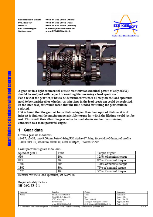
Customer Supplier ProjectDocument Public EES KISSsoft GmbH Weid 10, P.O. Box 121 6313 Menzingen Switzerland www.EES-KISSsoft.ch Title: -No.: -Date: 16.4.08Manager: Hanspeter Dinner@: h.dinner@EES-KISSsoft.chVersion: 0 Autor: HD Date: 16.4.08 Approved: HD Date: 16.4.08 EES KISSsoft GmbH ++41 41 755 09 54 (Phone)P.O. Box 121 ++41 41 755 09 48 (Fax)Weid 10 ++41 79 821 25 41 (Mobile)6313 Menzingen h.dinner@EES-KISSsoft.chSwitzerland www.EES-KISSsoft.chA gear set in a light commercial vehicle transmission (nominal power of only 35kW) should be analysed with respect to resulting lifetime using a load spectrum. For a test of the gear set, it has to be determined whether all steps in the load spectrum need to be considered or whether certain steps in the load spectrum could be neglected. In the later case, this would mean that the time needed for testing the gear could be reduced. If it is found that the gear set has a lifetime higher than the required lifetime, it is of interest to find out the maximum permissible torque for which the lifetime would just be met. This would then allow the gear set to be used also in another transmission, connected to a more powerful engine. 1 Gear data Given a gear set as follows: z1=17, z2=33, mn=3.00mm, beta=14deg RH, alpha=17.5deg, facewidth=20mm, ref profile1.40/0.30/1.10, a=78mm, x1=0.30, n1=1300RpM, Tnom=275NmLoad spectrum is given as follows:Speed of gear 1 Time Torque of gear 1650 10h 125% of nominal torque 975 20h 80% of nominal torque 1300 30h 100% of nominal torque 1300 30h 75% of nominal torque 1625 10h50% of nominal torque Because we use a load spectrum, set KA=1.00Required safety factorsSH=0.90, SF=1.1G e a r l i f e t i m e c a l c u l a t i o n w i t h l o a d s p e c t r u m2 Questions1)What is the resulting lifetime?2)What is determining the lifetime of the gear set (flank or root? gear 1 or gear 2?)3)Which load step contributes most to the damage of the gear4)If the gear set has to operate for only 1000h, what is the maximum nominal torque thatcan be transmitted instead of the 275Nm above?3 Solution3.1 Basic gear data input, definition of load spectrumStart with an empty file for all other settings not mentioned above.Enter basic gear data as follows:Enter the reference profile as follows:Go to database tool and open a new load spectrum definitionEnter the load spectrum as follows, then save the load spectrum:to select the load spectrum as shown below:The fact that a load spectrum is used can now be seen by the symbol as shown below:Now, define the required safety factors in the module specific settings:3.2 Answer to question 1)Finally, you can calculate the resulting life time by pressing next to the required lifetimeto find the resulting lifetime of 3223h3.3 Answer to question 2)We can now, based on the above lifetime, calculate the safety factors. Of course, the lowestsafety factor is now as specified in the module specific settings, required safety factors:In this example, the flank safety factor of gear 1 is equal to the required safety factor of 0.90.All other safety factors are higher than the required safety factors. This means the that flank ofgear 1 is the determining the lifetime of the gear set.3.4 Answer to question 3)Check in the report “Lifetime”There, you will find the partial damages for each load step in the load spectrum:The first step in the load spectrum contributes most, the third step is also important. The other steps contribute nothing to the total damage! This means that for example to test the gears, these load levels need not be tested at all!3.5 Answer to question 4)If the gear set has to run for only 1000h, it obviously can take more torque that the 275Nm specified above. You can calculate the nominal torque that can be transmitted (still considering the load spectrum) by entering the 1000h as a lifetime and then pressing the button next to the field for torque. Then, the nominal torque transmittable (considering the load spectrum), for a required lifetime of 1000h and for the required safety factors, will be returned, here with 311Nm:This means that the gear set could also be used in a transmission rated for slightly higher power rating than 40kW.。
Simtrix.simplis中文教程
Simetrix/Simplis仿真基础近4年开发电源的过程,在使用仿真软件的过程中,对仿真渐渐有了个了解,仿真不能代替实验。
仿真软件显示电路不能工作,而实际确能工作,仿真不收敛,而实际电路永远不会不收敛。
但是仿真软件可以测试未知电路,可以验证自己的想法,甚至大大缩短开发过程,在你仿真的过程中,也可以更深入的理解开关电源的拓扑结构,控制模式等,假如你要实验一个电路,发现库里没有现成的IC,在自己搭建IC之后,你对整个IC具体是如何运作的必定了解的非常清楚。
如果你的模型足够精确,你可以得到和实验室非常接近的结果。
如果你的电路是错误的,你也不用担心“炸机”的危险。
Simetrix/Simplis是我个人比较喜欢用的一款仿真软件,相对与功能强大的SABER, Simetrix/Simplis具有操作简单,容易上手,速度快等特点,用来实验开关电源的各个功能电路非常不错,精通之后,也能进行更复杂的仿真实验,比如开关电源的损耗分析,环路分析,大信号分析,IC设计等。
“只要你能想到的,你就可以用电路实现!”虽然这几年一直在接触这款软件,但离“精通”还相差很远,但我想利用它简单易学的特点,让更多的人了解使用它,对实际开发有所帮助。
并希望引出玉来,使大家共同提高。
我打算先说一下软件操作过程,再举几个简单的实例,供大家参考。
由于水平有些,只能说这些基础的东西。
先说一下目录1.基础操作:放置元件2.导入PSPICE模型3.瞬态分析,DC分析,AC分析,参数扫描4.自建子电路,元件库5.用SIMETRIX仿真开环BUCK。
6.用SIMPLIS 仿真BUCK电路:POP分析,AC分析。
7.两个简单的实例:桥式整流带恒功率负载—表达式的应用填谷PFC PF值计算-波形的分析和处理更深入一点的实例如电流模式反激电路。
准谐振反激电路。
单极反激PFC电路。
LLC电路等。
做好后会和大家分享。
1.放置元件。
先打开程序,点击File——New Schematic,建立新电路图点这两处地方可以放置元件基本的元件如DC电源,波形发生器电源,分段源,受控源,电阻,电容,电感,变压器,MOS管,三极管,二级管,稳压管,压控开关,地,电压探头,电流探头,运放等都能找的到,如上图,也可以从Place——From Model Library菜单中找到更多的元件,如3842,TL431等。
PS实例教程精品PPT课件

照片美容之去红眼
操作步骤:
(3)Ctrl D取消选区即可
照片美容之去明暗度调整
实例七:我们在拍摄照片的过程中,经常会
出现照片过亮,或者照片过暗的情况,我们通 常叫做曝光过度,或者曝光不足,利用ps也可 以轻松的完成照片的调整。
照片美容之去明暗度调整
操作步骤:
(1)打开需要调整的图片,该图片有些偏暗, 我们可以按住键盘的ctrl+J键复制背景图层。
选择编辑菜单下方的定义图案命令,将其定义为 图案
底图制作
操作步骤:
(5)新建一个文件,大小为210*297毫米,选择 编辑菜单下的填充命令,设置如下。
当尺寸设定完毕后,裁切后可以直接生成设定尺寸的图像。
倾斜照片校正
实例二:我们先看一张图片
整张照片因为拍摄的原因将大楼排成了倾斜的,不符合我们的正常的 是观看范围,如何利用ps软件将该建筑变成正常的呢?
倾斜照片校正
实例二:完成后的效果是
倾斜照片校正
操作步骤:
(1)利用ps工具的裁切命令 ,利用该工具将 整个照片进行裁切框选,勾选工具属性栏中的 透视命令复选框 然后将右上角的角点进行左移与楼的右侧边线 平行。
照片美容之去明暗度调整
操作步骤:
(4)ctrl+shift+s键, 保存成jpg格式的文 件。
汽车调色
实例八:利用ps的强大功能,可以快速的为
单色的物体进行颜色调整,我们先看下面的例 子。
汽车调色
操作步骤:
(1)打开汽车图片,选择 图像菜单下面的调整命令 中的替换颜色命令,利用 吸管工具在车上点击,并 在替换中更换为你需要更 改的汽车颜色。
将自己的证件照片设定成一个固定的尺寸和小 于多少k的尺寸,怎么用ps去实现呢?比如下 面一张图片,需要将其调整为:30K以内,宽 是114像素,高156像素。
kisssys入门实例教程3
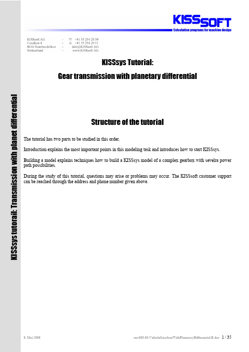
KISSsys Tutorial:Gear transmission with planetary differentialStructure of the tutorial The tutorial has two parts to be studied in this order. Introduction explains the most important points in this modeling task and introduces how to start KISSsys. Building a model explains techniques how to build a KISSsys model of a complex gearbox with sevelra power path possibilities. During the study of this tutorial, questions may arise or problems may occur. The KISSsoft customer support can be reached through the address and phone number given above.K I S S s y s t u t o r a i l : T r a n s m i s s i o n w i t h p l a n e t d i f f e r e n t i a l1Table of contents1 Table of contents (2)2 Introduction (4)2.1 Summary of the most important points (4)2.2 Systematicprocedure (4)2.3 Errata and remarks (4)task (4)2.4 ModellingKISSsys (5)2.5 Starting2.6 Selection of the project directory (5)2.7 Opening an empty KISSsys model (6)templates (6)the2.8 Loadingmodel (7)3 Buildingastructure (7)3.1 Treeelements (7)3.1.1 Machine3.1.2 Loads due to overlaid shafts (7)3.1.3 Connections (9)flow (12)3.1.4 Power3.1.5 Adding KISSsoft analysis modules (14)3.2 Input of Gear-, shaft- and bearing data (15)data (15)3.2.1 Gear3.2.2 Shafts and bearings (16)View (19)4 3D4.1 Adding 3D view in the tree structure (19)4.2 Location of the shafts (19)4.2.1 Positioning of the shafts s1a and s1b (19)4.2.2 Positioning of the shaft s2 (19)4.2.3 Positioning of the shaft s6 (20)4.2.4 Positioning of the shaft s3 (20)4.2.5 Positioning of the shaft s4 (20)4.2.6 Positioning of the shaft s5 (21)4.2.7 Positioning of the planet spindle (21)4.3 Work with the 3D Viewer (21)4.3.1 Inside diameters of the gear wheels (21)4.3.2 Color and transparency (22)4.3.3 Visualizing bearings in a shaft bore (22)4.4 Insert data from CAD system (23)5 Changing of gears (24)5.1 Background Information about clutch elements (24)5.2 Applied in the current example (24)5.3 Start of the function (26)Interface (27)6 User6.1 Input of the power (27)6.2 Execute buttons for function in the User Interface (28)model (29)the7 Completing7.1 Calculation of the bearing speed in system with overlaid shafts (29)7.2 Input of the speed ratio for front and rear drive (30)7.3 Input of efficiency (31)7.4 Settings to calculation methodology (32)tooth contact of a gear wheel (32)multiple8 Calculationof8.1 Remarks (32)8.2 Calculation on-road and off-road gear selection (32)8.3 Functionality (33)9 Annex A, ...Set Speed“ (35)9.1 Code (line numbers are not part of the code) (35)9.2 Clarification (35)2Introduction2.1Summary of the most important points1)Where two or more shafts overlap, the bearing load from the around shaft must be transferred by a forceelement to the shaft which is under it. (see chapter 3.1.2)2)For this transfer of bearing loads from one coaxial shaft to the other, …call ‘OnCalcTorque’ duringcalculation of torque” has to be activated. (see chapter 7.4)3)Further, the relative speed of the bearings between overlaid shafts must be calculated as the differencein speed between bearing outer ring and bearing inner ring. (section 7.1)4)The speed at the two output shafts (front and rear axle) are placed with one to another in reference.Therefore the speed at one output shaft has to be set as "Constraint=Yes" and an expression is set to compute one speed (those of the front axle) from the other (the rear axle). In addition, an iteration is necessary for the calculation of the relative speed) ( section 3.1.2 and 7.1)5)"Iteration for torques” and “speed with damping" must be set to execute the iteration. (Section 7.4).2.2Systematic procedureThe following steps are involved when building a KISSsys model:1.Planning: Naming, range and goals of the model2.Insert mechanical component in the tree structure (red Icons)3.Connect mechanical component to each other (grey Icons)4.Define sources of power flow5.Add KISSsoft calculation to the mechanical components (blue Icons)6.Add 3D graphic, and position elements in the graphic7.Add tables / User Interfaces8.Program own functions9.Tests, debugging2.3Errata and remarks1)If questions or difficulties arise during the tutorial, KISSsoft Hotline can be used for assistance (e-mailaddress, tel. no. etc. see front of document).2)The planetary differential used for this example in practice would be a double planet planetary wherethe sun and the planet carrier have the same sense of rotation. However, to prevent the example becoming too complex, a simple planetary train is used. Therefore both outputs rotate contrary to each other.3)The original idea for this tutorial had planned a differential lock between the annulus and the planetcarrier. This clutch is called c3. In reality it will be not used although in the tutorial it is described. It is recommended to proceed exactly according to the tutorial instructions (i.e. the clutch c3 is to be modeled although this is not used).4)An error occurs with the nomination of the forces on s2 due the overlap of shaft s6.2.4Modelling taskA transfer gearbox for a 4x4 off-highway vehicle is to be modeled. The transmission possesses an on- and off -road gear as well as a lockable epicyclic differential acting as a longitudinal differential. A part of the power is continually taken off over a PTO. The bevel gear differentials in the axles are not modeled. The unlocked gears z1 and z2 on the input shaft clutches can be switched on or off.Figure2.4-1 Sketch of the gear train to be modeledFollowing names and characters are useds = shaft; z = gear; c = clutch/couplings; b = bearing (b1: left side bearing, b2: right side bearing) red arrow is power input respective power outputred arc is power transmitted through virtual coupling c32.5Starting KISSsysFirst, a project folder has to be created. Then, KISSsys 03/2008 is to be started and the intended folder is chosen as project folder.Using “Options”, activate the administrator mode. Then, the templates should be opened using “File/Open templates…”.Make sure the latest Patch version is installed on your computer. (Download from www.KISSsoft.ch)2.6Selection of the project directoryKISSsys works with so called ‘projects’ to manage the files. These are listed directory names, in which the KISSsys model and pertinent KISSsoft files are stored. Before a model can be opened in KISSsys, a directory must be defined in which the KISSsys model is to be stored. Therefore a new appropriate directory name has to be created in the main directory KISSsys before starting to model.Through the button in the red marked circle the new directory can be selected. Please notice, the appropriate directory shows up only if you have created the directory as described in the sentence above. In our case: C:\Programme\KISSsoft 03-2008\KISSsys\tutorial-003. After the selection of the directory in the Windowsdialogue with "opening" is to be confirmed, press “open” and KISSsys is launched.Figure2.6-1 Selection of the project directory2.7Opening an empty KISSsys modelKISSsys starts now with an empty model. As a first step, the "administrator" mode must be activated under themain menu "Options".Figure2.7-1 Activate the administrator mode under “Estras” in the main menuIf the option "administrator" can not be selected, then the KISSsys license is missing. In this case contactKISSsoft AG.2.8Loading the templatesAs a first step when creating a new KISSsys model, the templates are to be imported through the menu “File”,“Open templates…”, “templates.ks”. In the templates, all elements are now listed which can be used inKISSsys:Figure2.8-1 Element library … Templates“.After having imported the templates, the model can now start to be built.3Building a model3.1Tree structureIn a first step all existing mechanical components must be defined in a tree structure. It is highly recommended to name gears, shafts, bearings and couplings in such a way as shown in the illustration down. User can define first shaft (e.g. “s1” with bearings “b1 and “b2”) and then copy it to avoid adding all bearings one by one.3.1.1Machine elementsFigure3.1-1 Shafts, Shafts with bearings, shafts with bearings /couplings, elements for modeling epicyclic gear trains The same names can be used several times for different mechanical components, as long as the mechanical components are in a different path of the tree. Please note all bearings are called "b". The left hand bearing is "b1"; the right hand bearing is "b2".The following is important when modeling an epicyclic gear train:1)The planet is supported only by one bearing. I.e. on the shaft …sp“ there is only one bearing…b1“(…kSysRollerBearing“ from the templates) placed.2)The planet carrier needs a special coupling: ”kSysPlanetCarrierCoupling“. Do not mix up this elementwith …kSysCoupling“. This special coupling should be named as …cc“ and will be positioned on the shaft s5. This element is necessary to rotate the planet in the world coordinate system.After these two elements are added, the tree structure looks like in illustration 3.1-1 (above right).All spur gears must be arranged on the respective shafts, the tree structure looks as follows in Figure3.1-53.1.2Loads due to overlaid shaftsForce elements on the shafts “s1” and “s2” have to be added. These force elements are to lead the bearing loads of “s1a” and “s1b” as well as “s6“ in each case on those under it lying shaft (s1 and s2). From the templates the element "kSysCentricalLoad" is used. Four forces are used in total on “s1”, on “s2” two forces are applied. The names of these forces should identify the origin of the force.The names of the forces expose themselves together:For example …f_s1ab1“:…f“ for force…s1a“ marks the shaft that the force is taken over…b1“ marks the bearing that the load is taken overFigure 3.1-2 Forces due to the overlaid shafts on s1 and s2The force components of the inserted forces must be connected with the components of the bearing loads. To do this the right mouse button must be clicked on a force (e.g. f_s1ab1), whereupon the "characteristics" (Properties) appear and must be selected, and after selecting “Fx” under “expression” the following text has to be inserting: GB.s1.s1a.b1.Fx.The expression makes sure the load on the shaftaffecting the load on the other shaft (respectivelytheir x-component) equals the x-component of thebearing load b1 on s1a.The appropriate expressions must be registered alsofor Fy, Fz, Tx and TzFor Fy: GB.s1.s1a.b1.FyFor Fz: GB.s1.s1a.b1.FzFor Tx: GB.s1.s1a.b1.MxFor Tz: GB.s1.s1a.b1.MzThese linkages of the forces must be done for allforces provided:f_s1ab1, f_s1ab2, f_s1bb1, f_s1bb2, f_s6b1, f_s6b2.Figure 3.1-3 Linking force componentAdd as well automatic positioning for the forces on the shaft according to the positions of the bearings. For thisuse functions l_p() to set positions.The expression makes sure the load position on the shaft isequal to the position of the mating bearing (respectively theiry-component).This function looks for reference element and point on parentelement and converts coordinates. Finally only y-direction istaken (*{01,0})l_p(GB.s1.s1a.b1,{0,0,0})*{0,1,0}The appropriate expressions must be registered also for allother forces.Figure 3.1-4 Linking force positionsFinally add gear components to the model.Figure3.1-5 Tree structure and KISSsys sketch with mechanical components3.1.3ConnectionsIn the next step the following connections are defined:1)Connections of the shift clutches for the road gear (c1, c1): It uses "kSysCouplingConstraint" from thetemplates.Action:First copy from the templates "kSysCouplingConstraint" and paste it to the tree structure within the group "GB". The name will be specified with "C1", thus it is clear which clutches are connected (namely c1 on s1 with c1 on s1a). In a second step the clutches which can be connected are to be selected. In addition it must be defined whether the clutch is closed (activated) or open (not activated).Figure3.1-6 Definition of a clutch connection, here for road course2)Connect the shift clutches for the off road gear (c2, c2). This clutch will be open.(…Activated=No“)because both gears can not be closed at the same time:Figure3.1-7 Definition of the clutch for off road course3)Connect both clutches c3, differential lock. The clutch will be open (…Activated=No“):Figure3.1-8 Connection between clutches c3After all clutches are connected within the transmission, the individual gears must be connecting together. For the spur gears, the type "kSysGearPairConstraint" is necessary. The planets need the type “kSysPlanetaryGearPairConstraint " two times. One where the sun wheel connects the planet, the other the planet connects the annulus. The connections are copied from the templates into the tree structure, below the group of "GB":Gear pair gp1 Gear pair gp2Gear pair gp3 Gear pair gp4Figure3.1-9 Definition of gear pairs.Gear pair sun zs between Planet zp “sp”Gear pair planet zp between annulus zr “pr”Figure3.1-10 Definition of a planet gear connection in the systemThe tree structure with the connections defined in the KISSsys sketch should look now as follows:Black line connections: active / close connectionsGrey line connections: inactive / open connectionsFigure3.1-11 Tree structure and KISSsys sketch with connections3.1.4 Power flowThe definition of the power flow in the gearbox is through the element …kSysSpeedOrForce“. This element is to be copied from the templates and pasted four times directly into the tree structure (not under …GB“)During the power input "Input" speed and the torque are given. Both values are signed sizes. If the product of the two signs is positive, then the power is positive, i.e. it concerns a positive input power.Figure3.1-12 Definition of Input power …Input“(Motor)The PTO torque is set to 10Nm (acceptance for this example). The direction of rotation is counter clockwise. The number of revolutions is therefore negative. The torque has to be entered positively thereby the power output becomes negative.Figure3.1-13 Definition of the power take off (PTO)Rear-wheel drive RWD (OutR)As a consequence, number of revs and torque follows by the input data and the type of transmission. No values are given.Figure3.1-14 Definition of the RWDFront wheel drive FWD (OutF)The condition for the front wheel drive is defined as follows:Front axle and rear axle turn with the same speed, but contrary. This condition will be still specified in section 7,2.Thus the number of revolutions at this output (the front axle) is the same as from the number of revolutions of the output “OutR", therefore "speed of constrained=yes" must be set.With the right mouse-click on the power output "OutF" and the choice in "Properties" of "speed", an expression for the speed can be defined at this output. Enter in the field "Expression":"-OutR.speed". This guarantees that the speed at the output is equal the speed of the shaft s5, but in opposite direction of rotation.Figure3.1-15 Definition of the FWDNow the kinetic calculations can be started using right mouse-clicks on menu, selection of "Calculate Kinematics". (Section 7.4 must also be considered). After a Refresh, the sketch looks as follows:Figure3.1-16 KISSsys model with power flow after execution of kinematics analysis3.1.5Adding KISSsoft analysis modulesNext step is to introduce the KISSsoft analysis modules. These are copied from the templates. KISSsoft analysis modules for shafts, bearings and gears are needed. The gear pair and planetary gear analysis are arranged directly below the appropriate connection with the same name. The shaft and bearing calculations are inserted within the appropriate shaft computation.The bearing calculation "Bearing2" is copied from the templates. The index "2" means that altogether two antifriction bearings are computed. Note: for the planet “Bearing1" must be used from the templates since the planet is stored on the spindle only through an antifriction bearing. Bearing calculations can be also done directly in shaft module, but in cases when bearings are between two shafts separate calculation modules should be used to set speed for bearing correctly (relative speed between two shafts).Figure3.1-17 Tree structure with computations (left), and templates used (right)3.2Input of Gear-, shaft- and bearing data3.2.1Gear dataThe following teeth data in Figure 3.2 is used in this example. In addition double-click on the computations (blue Icons) in the tree structure. After entering the design data, the input in each case has to be confirmed with"calculation F5". Afterwards, close the KISSsoft window with "exit" (cross in the right upper corner).Figure3.2-1 Input data gear pair gp1 Figure3.2-2 Input data gear pair gp2Figure3.2-3 Input data gear pair gp3 Figure3.2-4 Input data gear pair gp4Figure3.2-5 Input data for epicyclic drive train3.2.2Shafts and bearingsPosition of elements cIn: y = 5 mm c1: y = 70 mm c2: y = 140 mmPosition of bearings: y = 15 mm y = 170 mmPosition of gear z6: y = 190 mmFigure3.2-6 Input data shaft s1Position of gears: z2 y = 50 mm z4 y = 120 mmPosition of bearings: y = 15 mm y = 195 mmFigure3.2-7 Input data shaft s2Position of the clutches: y=28 mm for s1a, s1b and s6Position of the gear 15 mm Position of bearings 5 mm and 25 mmFigure3.2-8 Input data s1a, s1b, s6Coupling: cc y = 5mmcrOut: y = 190 mm c3: y = 70 mmBearings 90 mm and 170 mmFigure3.2-9 Input data s5coupling cfOut: y=10mm, zs: y=190Bearings 30 mm and 150 mmFigure3.2-10 Input data s4Figure3.2-11 Input Planet pin (sp)To calculate shaft with only one support it may be necessary to activate calculation with bearing internal geometry.z5: y =10mm zr: y = 20mmclutch c3: y=65 mm b1: y = 30 mm b2: y = 58 mmFigure3.2-12 Input data s343D View4.1Adding 3D view in the tree structureFrom the templates, the 3D view "kSys3Dview" is inserted into the highest level of the tree structure. Select “show" using right mouse button by touching the insert function. All mechanical components are still in the same position because their position in the working sheet is not defined. Therefore, the next step will be to arrange the positions of the shafts in the coordinate system.Figure4.1-1 3D view of the gear train model4.2Location of the shafts4.2.1Positioning of the shafts s1a and s1bThe shafts “s1a” and “s1b” are positioned in reference to shaft “s1”. The shafts have a radial distance of zero, and axial length of 35mm and 105mm for “s1a” and “s1b” respectively on shaft “s1”.Figure4.2-1 Positioning of the shafts s1a and s1b to s14.2.2Positioning of the shaft s2The shaft s2 is positioned relative to shaft s1. Both shafts s1 and s2 end at the same horizontal X-position. The distance between the two shafts is equal to the centre distance (a) of the gear pair gp1. (or gp2; or gp4)Figure4.2-2 Positioning of the shaft s24.2.3Positioning of the shaft s6The shaft s6 is positioned relative to shaft 2 (s2). The radial distance is zero. The relative Y-position to the shaft s2 is delta y=180mm.Figure4.2-3 Positioning of the shaft s64.2.4Positioning of the shaft s3This shaft must be placed such that both gears “z5” and “z4” are touching each other through both centre lines of the facewidth. Shaft “s3” has to be placed relative to “s2”. The distance is exactly the centre distance between gear pair “gp3”. The y-position is defined by the position of both gears. The location of the gears on the shaft itself is stored in the variable …position“. Furthermore, the shaft “s3” is located vertically below the shaft “s2”. (phi = -90 deg)Figure4.2-4 Positioning of the shaft s34.2.5Positioning of the shaft s4The shaft “s4” is positioned in reference to shaft “s3”. Both are concentric to each other. The relative Y-position must be chosen in a way that the centre-line of both the gear “zr” on the shaft “s3” and gear “zs” on the shaft “s4” have the same absolute Y-value.Figure4.2-5 Positioning of the shaft s44.2.6Positioning of the shaft s5The shaft “s5” is positioned in reference to the shaft “s3”. They have the same centre line. The relative y position must be selected in such a way that “zp” gear (planet) and “zr” gear (annulus) are on the same absolute y position. The right shaft end of the planet spindle is in the same position as the left shaft end of “s5”. The distance from the centre of the planet to the end of planet spindle is 5mm.Figure4.2-6 Positioning of the shaft s54.2.7Positioning of the planet spindleThe planet spindle is positioned in reference to the shaft “s3”. The planet and the annulus have the same Y-position. The centre distance is given through the KISSsoft gear calculation of the gear stage.Figure4.2-7 Positioning of the planet spindlePress “Refresh” button on menu to see all components places correctly in the space.4.3Work with the 3D Viewer4.3.1Inside diameters of the gear wheelsThe inside diameters of the gear wheels should be set equal to the outside diameter of the respective shaft. For all gear wheels, except the internal gear, the variable “di” should have the following text inserted in the field “expression”:Figure4.3-1 Expression for (i)This supplies the outside diameter of the shaft at the place where the gear part is located.For the internal gear zr, the value for "di" must be inserted manually (in the field "value") equal to the inside diameter of the shaft, but negative:Figure4.3-2 Insert of …di“ by the internal gear zr4.3.2Color and transparencyA variable “kSys_3DColor” and “kSys_3Dtransparency” can be affixed to the mechanical components (gear wheels "z", bearings ”b”, shafts "s" and clutches "c"). This will change the colour and transparency of the selected element. Numerical values 0-255 change the colors, while for transparency between select obscure (0) to transparent (1). User can also use setting functionality from the menu to set colors and appearance for the components.Figure 4.3-3 3D graphic settings4.3.3Visualizing bearings in a shaft boreThe following trick must be used to set correct visualization for the bearings defined according to internal geometry. For both bearings on the shafts “s1a”, “s1b” and “s6” from the variable "d" under “Properties” expression must be deleted for each case.The expression from “d”need to be deletedFigure4.3-4 Necessary …Trick“ for visualizing bearings in a shaft boreAfter a refresh command, the 3D view looks like the following:Bearing: green.Shaft with the non-locater bearing: grey, obscure.Underlying shaft: grey, transparentAlso shown: The local coordinate system from thesame shaft.Figure4.3-5 Correct view of the bearing4.4Insert data from CAD systemDepending upon version of KISSsys *.sat, *.iges or *.step data from any CAD system can be imported. In addition, "kSysCasing" has to be copied from the templates into the tree structure. In this example, four individual CAD data records are read in, and four KISSsys elements of type "kSysCasing" are created. They are called in this example "Wheel1" to "Wheel4": The file attached in this example is called “tut-003-CAD-data.igs”Figure4.4-1 Tree structure with inserted elements for the integration of the CAD data (left), dialogue to “kSysCasing” elements (right)If the dialogue window is open by the right mouse button, then under “Type”” Read file” must be selected. In the field "file name" the complete file name inclusive path is to be indicated if file is not in located in the project folder. Positioning of the Wheels can be done manually entering in the Properties and changing position values.After a refresh the 3D view can look as follows:Figure4.4-2 3D view of the transmission gearbox with imported geometry5 Changing of gears5.1 Background Information about clutch elementsFor the clutch connection the function:setConfig(Activation,Torque constrain)There are the following usual cases:• Clutch is closed, no slip, torque is calculated: setConfig([TRUE, 0], FALSE)• Clutch is closed, slip and torque is given: setConfig([TRUE, slip], [TRUE, moment]) • Clutch is open, no torque: setConfig(FALSE, FALSE)• Clutch is open, torque is given: setConfig(FALSE, [TRUE, moment])For a transmission with two gears, with a given torque at the output in the first gear and given torque at the input by the second gear, a changing gear function can look as follows: (Note! This is only example code)IF gear=1 THEN Coupling1.setConfig([TRUE, 0], FALSE); Coupling2.setConfig(FALSE, FALSE); Input.setConfig(TRUE, FALSE); Output.setConfig(FALSE, TRUE); ELSIF gear=2 THEN Coupling1.setConfig(FALSE, FALSE);Coupling2.setConfig([TRUE,0], FALSE);Input.setConfig(FALSE, FALSE);Output.setConfig(TRUE, TRUE);ENDIFCheck if gear 1 is connected. Set clutches according to the gear selection Set boundary conditions If gear 2 selected do settings according to that 5.2 Applied in the current exampleThe function for changing gears should be contained in a table "Settings". First from the templates the table "user interface" must be copied into the highest level of the tree structure. The table has to be named "Settings". Using the right mouse button, the size of the table can be defined under "dialogue". The table can be visualized by selecting "show". Using the right mouse-click under "Settings" in the tree structure, on selection of "new variable" a further variable with the name "SetSpeed" of the type "function" can be insert.By the right mouse-click on "Settings" and the selection of …Properties", the following window opens. Now the function editor can be called by the right mouse-clicks on "set speed" and the selection by "Edit".Further, a variable "OnOffRoad" of the type "real" is to be added. This will describe the momentarily selected gear. If it is 0, then the on-road gear is active, and if 1 then the off-road gear is engaged.Figure5.2-1 Properties (different variables) under …Settings“. NOTE: the new variables OnOffRoad, Set Speed appeared.Figure5.2-2 Function …Set Speed“ (NOTE:more details about this in Annex A)The function "CADH_VarDialog" generates a dialogue in which can be defined whether the on- or off- road gear is selected. The dialogue supplies an array of "res" as result. Zero elements into "res" is 1 (or TRUE) if the dialogue is confirmed using "OK", 0 (or FALSE) if the dialogue is closed with "CANCEL". The first element of the array corresponds to the selection made. If "on-Road" is selected then 0 is returned, otherwise "off Road" is selected and 1 is set.The first “IF” condition examines if the dialogue was closed with "OK". After this the selection is put into the variable “Settings.OnOffRoad”. If "on-Road" was selected, the clutch “C1” is closed, “C2” is open. If "off Road" was selected, the clutch “C2” is closed, and “C1” is open. Next, the kinematics calculation is called to calculate new power flow. The function can still be extended so that the open clutch in the 3D diagram is translucently represented, the closed clutch obscurely:Figure5.2-3 Function …SetSpeed“。
2024年kisssoft齿轮培训

kisssoft齿轮培训KISSsoft齿轮培训:掌握现代齿轮设计分析技术的关键引言随着工业技术的不断发展,齿轮作为机械传动系统中的核心部件,其设计、制造和分析的精度和效率显得尤为重要。
KISSsoft是一款专业的齿轮设计和分析软件,它为工程师们提供了一套完整的工具,用于精确计算和模拟齿轮传动的各种性能。
本文旨在介绍KISSsoft齿轮培训的重要性,以及如何通过培训掌握这一现代齿轮设计分析技术。
第一部分:KISSsoft齿轮培训的重要性1.1齿轮设计分析的挑战齿轮设计分析是一个复杂的过程,涉及到多种学科的交叉应用,包括力学、材料科学、热处理技术等。
随着工业产品对性能和可靠性的要求越来越高,传统的齿轮设计方法已经无法满足现代工业的需求。
1.2KISSsoft软件的优势KISSsoft软件以其强大的计算引擎和用户友好的界面,在齿轮设计分析领域得到了广泛的应用。
它能够帮助工程师快速、准确地完成齿轮的几何设计、强度校核、接触和弯曲疲劳寿命预测等工作,大大提高了齿轮设计的效率和质量。
1.3培训的必要性虽然KISSsoft软件功能强大,但要充分发挥其作用,需要用户具备一定的专业知识和操作技能。
因此,参加KISSsoft齿轮培训,系统学习软件的使用方法和齿轮设计分析的理论知识,对于提高工程师的专业能力,提升企业产品的竞争力具有重要意义。
第二部分:KISSsoft齿轮培训内容2.1软件基本操作KISSsoft齿轮培训会教授软件的基本操作,包括软件的安装、界面布局、菜单功能等。
通过这部分的学习,学员能够熟悉软件的操作环境,为后续的学习打下基础。
2.2齿轮设计原理培训将详细介绍齿轮设计的基本原理,包括齿轮的几何参数、啮合原理、齿面接触分析等。
这部分内容是理解和使用KISSsoft软件进行齿轮设计的基础。
2.3齿轮强度计算强度计算是齿轮设计中的关键环节。
培训将教授如何使用KISSsoft软件进行齿轮的接触强度和弯曲强度计算,以及如何根据计算结果优化齿轮设计。
KISSsoft软件基础培训

04
轴承设计基础
轴承类型及特点
滚动轴承
包括球轴承、滚子轴承等, 具有高转速、低摩擦、长 寿命等特点。
滑动轴承
包括整体式滑动轴承、剖 分式滑动轴承等,具有承 载能力强、刚度高、耐冲 击等特点。
特殊轴承
如磁悬浮轴承、气浮轴承 等,适用于特殊场合,具 有高精度、高稳定性等特 点。
轴承的选用与校核
选用原则
轴的结构设计与优化
01
便于加工和装配。
02
结构优化方法
合理选择截面形状和尺寸,以减小应力集中。
03
轴的结构设计与优化
01
采用空心轴、改变材料等方法减轻 重量。
02
优化轴承和键槽设计,提高轴的承 载能力和传动效率。
轴的强度校核与疲劳寿命分析
强度校核方法
1
计算轴上的载荷和弯矩。
2
3
根据轴的材质和截面尺寸计算许用应力。
半圆键连接
适用于轻载连接,常用于锥形轴端与 轮毂的连接。
楔键连接
适用于定心精度要求不高、载荷平稳 和低速的场合。
花键连接的类型及特点
矩形花键
齿数多,承载能力强,对中性好,导向性好,但 加工成本高。
渐开线花键
齿数少,齿根厚,承载能力强,易加工,但导向 性较差。
三角形花键
齿数适中,承载能力较强,加工方便,但导向性 一般。
齿轮参数计算与选择
模数选择
根据齿轮所受载荷和转速选择合 适的模数。
压力角选择
一般选择20°或15°压力角,也可 根据特殊需求选择其他角度。
齿数选择
避免根切和齿顶变尖,同时考虑 传动比和中心距要求。
其他参数
如螺旋角、变位系数等,根据具 体需求进行计算和选择。
kisssoft-tut-001-C-安装试用和初始步骤
KISSsoft 03/2014 –教程1 安装试用和初始步骤KISSsoft AGRosengartenstrasse 48608 BubikonSwitzerlandPhone: +41 55 254 20 50Fax: +41 55 254 20 51info@KISSsoft.AGwww.KISSsoft.AG目录1.安装 (3)1.1.使用须知 (3)1.2.安装 (3)1.3.激活试用版本 (3)1.3.1情况1:通过许可证代码在线激活 (3)1.3.2情况2:用激活码激活软件 (4)2.启动 KISSsoft (5)2.1.启动软件 (5)2.2.启动计算模块 (5)2.3.打开现成案例 (6)3.如何使用KISSsoft (7)3.1.按钮 (7)3.2.帮助 (7)3.3.教程 (8)4.附带信息 (9)4.1.激活或者关闭单独的模块 (9)1. 安装1.1. 使用须知KISSsoft的演示版本虽然没有使用期限的限制,但是操作者却不能用它存储数据,及从下拉菜单中选择数据等,同时涉及到轴计算及圆柱齿轮计算流程的一些参数也已经被限制了。
尽管如此,,演示版本仍给关注者以“视觉和感官”的深刻印象。
然而遗憾的是,演示版不能被激活和安装任何补丁。
当然,试用版本是从演示版本开始激活。
为确保用户可以使用所有功能,首先必须在名为“Activating the test version”标签栏中(询问激活代码)激活软件,用户就可以有30天的时间来详细了解软件的所有功能并对软件进行评估。
在此期间,软件中所有的功能模块都开放使用,30天后,试用版本会自动变回演示版。
如果用户有任何问题都可联系KISSsoft公司的热线电话+41 55 254 20 53或者邮箱info@KISSsoft.AG,我们工作人员将热忱解答客户的任何疑问。
用户也可以登陆www.KISSsoft.AG官方网站了解KISSsoft软件的最新发展动向及操作详情等。
Surfer11最新版中文教程_图文
Surfer11 最新版中文教程_图文一、Surfer11 教程.................. . (1)第一课预览及创建数据 (3)第二课创建网格文件 (9)第三课创建等值线图 (14)第四课修改数轴 (27)第五课散点图数据点和图形图层的使用 (32)第六课创建一个剖面图 (48)第七课保存图形 (50)第九课增加透明度,色阶和标题 (58)第十课从不同的坐标系中创建图形 (63)第十一课自定义工具栏和键盘命令 (68)第十二课叠加图形层 (71)第十三课白化一个网格文件 (75)第十四课在工作表中更改投影 (79)二、汉化历程 (82)三、答疑解惑 ......................................................................... 89 CUPB第八课创建一个3D 曲面图 (52)一、Surfer 11教程程贤辅翻译 2012.10.20Surfer11版的帮助里面有一套非常好的教程,我希望能将它介绍给大家。
对于某些高手,可以也应该绕开,以免浪费您的宝贵时间。
其他朋友,如果您看了以下的教程,对您有帮助,那我就很高兴,也算我为我国的气象事业间接作了一点贡献。
该套教程共有14课,1到10 是初级教程,11到14是高级教程:1、预览及创建数据;2、创建网格文件;3、创建等值线图;4、修改坐标;5、散点图数据点和图形图层的使用;6、创建剖面图;7、保存图形;8、创建3D曲面图形;9、添加透明度、比色刻度尺和标题;10、从不同的坐标系统创建各类图形;11、自定义工具栏和键盘命令;12、覆盖图形层;13、白化一个网格文件;14、更改工作表中的投影。
我不知道我能不能完成所有的教程翻译工作,因为各种不可预计的因素会影响工作的进展。
尽量做吧。
想起40年前我为了制作一张等值图,要花费3天时间,用掉多少草稿纸和橡皮擦,要画出平滑的等值线还真不容易。
SIWSHMAX教程
SIWSHMAX教程第一章:快速入门篇A01 swishmax操作界面介绍A02 建立第一个文字特效影片文件(movie):点击输入文字(修改大小、颜色等)——选添加效果(效果可选取多个)——保存A03 swishmax软件应用的观念A04 停格的手法A05 更替文字(演员)的用途(不同层上文字输入效果)A06 文字基本设定A07 阴影效果的制作(在2个层上输入相同文字,选用不同颜色)A08 影片超链接的设定A09 汇入位图形(插入图片)A10 对象上下顺序的调整A11 效果复制,多个对象同时套用同一效果A12 五项基本工作流程:字体——修改颜色大小——文字效果——保存——导出A13 Movie(影片)、Scenes、Timeline & frame (多个场景、时间轴、影片)A14 Templates(范本)(模板,预设好的尺寸)第二章:新功能介绍一.scripting(程序撰写)B01 进阶scripting编辑接口:2个效果,第一个效果后有停顿,并继续播放后一个效果)在第一层输入文字——添加效果(2个)——在第二层(如第10帧)增加脚本(事件——帧(onFrame从第10帧开始,然后事件——影片控制stop)——回到第一层选中文字在第增加脚本(事件——按纽on press,事件——影片控制play)B02 除错debug功能:在第一帧添加脚本,事件——帧onlad(进来做什么),然后选调试trace追踪)此时显示红色,说明有误;选专家,在trace()括号中输入文字,切记要加双引号即trace(“文学”),输入后文字变成兰色,点播放影片,在右侧出现文学二.effects(特效)B03 超过230个内建特效:特效功能强大,有230个特效B04 可以自订特效并予以储存:即自己可以添加一些喜欢常用的文字效果点击T输入文字——添加效果(如墨西哥飘动),然后双击(在时间轴特效)处,出现对话框,可调整里面的设置及颜色,然后保存,它就会自动添加到文字特效中,以便下次使用B05 特效一次可以套用给多个对象三.drawing(绘图)B06 输入文字和动态文字功能:文字有三种即静态、动态、输入文字文字——文字静态——主要用来做特效文字——输入文字——名称可随意写(如第一层),可以修改格式、颜色等,主要是对输入文字的内容能直接修改,一般选格式——进阶文字——动态文字——名称(如歌词层)——脚本,事件——帧(如在第10帧)onfrane10——点专家在onfrane10后面的大括号中输入:歌词层=“变换”,既当影片播放到第10帧时原来的文字就会变为变换;如要在第1帧改变文字,则脚本,事件——点专家,将上一步内容,即onfrane10歌词层=“变换”复制,放到最前面,改为onfrane1歌词层=“开始”,然后点影片播放,在第1帧、第10帧文字会发生变化。
Surfer11最新版中文教程_图文
Surfer11 最新版中文教程_图文一、Surfer11 教程.................. . (1)第一课预览及创建数据 (3)第二课创建网格文件 (9)第三课创建等值线图 (14)第四课修改数轴 (27)第五课散点图数据点和图形图层的使用 (32)第六课创建一个剖面图 (48)第七课保存图形 (50)第九课增加透明度,色阶和标题 (58)第十课从不同的坐标系中创建图形 (63)第十一课自定义工具栏和键盘命令 (68)第十二课叠加图形层 (71)第十三课白化一个网格文件 (75)第十四课在工作表中更改投影 (79)二、汉化历程 (82)三、答疑解惑 ......................................................................... 89 CUPB第八课创建一个3D 曲面图 (52)一、Surfer 11教程程贤辅翻译 2012.10.20Surfer11版的帮助里面有一套非常好的教程,我希望能将它介绍给大家。
对于某些高手,可以也应该绕开,以免浪费您的宝贵时间。
其他朋友,如果您看了以下的教程,对您有帮助,那我就很高兴,也算我为我国的气象事业间接作了一点贡献。
该套教程共有14课,1到10 是初级教程,11到14是高级教程:1、预览及创建数据;2、创建网格文件;3、创建等值线图;4、修改坐标;5、散点图数据点和图形图层的使用;6、创建剖面图;7、保存图形;8、创建3D曲面图形;9、添加透明度、比色刻度尺和标题;10、从不同的坐标系统创建各类图形;11、自定义工具栏和键盘命令;12、覆盖图形层;13、白化一个网格文件;14、更改工作表中的投影。
我不知道我能不能完成所有的教程翻译工作,因为各种不可预计的因素会影响工作的进展。
尽量做吧。
想起40年前我为了制作一张等值图,要花费3天时间,用掉多少草稿纸和橡皮擦,要画出平滑的等值线还真不容易。
- 1、下载文档前请自行甄别文档内容的完整性,平台不提供额外的编辑、内容补充、找答案等附加服务。
- 2、"仅部分预览"的文档,不可在线预览部分如存在完整性等问题,可反馈申请退款(可完整预览的文档不适用该条件!)。
- 3、如文档侵犯您的权益,请联系客服反馈,我们会尽快为您处理(人工客服工作时间:9:00-18:30)。
许用材料的屈服强度(刚度)与各种应力的关系一 拉伸钢材的屈服强度与许用拉伸应力的关系[δ ]= δu/n n为安全系数轧、锻件 n=1.2—2.2 起重机械 n=1.7人力钢丝绳 n=4.5 土建工程 n=1.5载人用的钢丝绳 n=9 螺纹连 N=1.2-1.7铸件 n=1.6—2.5 一般钢材 n=1.6—2.5二 剪切许用剪应力与许用拉应力的关系1 对于塑性材料 [τ]=0.6—0.8[δ]2 对于脆性材料 [τ]=0.8--1.0[δ]三 挤压许用挤压应力与许用拉应力的关系1 对于塑性材料 [δj]=1.5—2.5[δ]2 对于脆性材料 [δj]=0.9—1.5[δ]四 扭转许用扭转应力与许用拉应力的关系:1 对于塑性材料 [δn]=0.5—0.6[δ]2 对于脆性材料 [δn]=0.8—1.0[δ]kisssoft销连接分为四个类型的计算,取决于使用它的地方。
与其它连接相比(花键、平键)可以做到零侧隙传动。
The bolt/pin connections are divided into four types of calculation depending on where they are used:这个螺栓/销连接分为四个类型的计算取决于使用它的地方。
2.2 横向销轴与轴套之间径向穿销连接。
横穿销结构加工方便,不受轴与轴套材料硬度不同的影响。
注意它不适合轴与轴套间大的间隙配合,以免销承受剪切以外的其他类型的外力。
例:交替作用扭矩20Nm,轻微冲击,轴与轴套配合半径30mm,轴套直径50mm,求配销最小配销直径?解:T=20Nm,载荷类型=alternating,KA=1.25,dw=30,S=(50-30)/2=10。
使用GB119.2圆柱销,材料为45#钢。
打开KISSSFOFT界面,进入圆柱销单元。
如图2.2所示输入参数。
图2.2单击自动调整按钮,软件会根据载荷大小自动给出销的最小直径,取整数4。
求解,单击工具条求解按钮,如图2.3所示。
图2.3单击生成报告按钮,软件给出计算结果如下:Results/结果:Pin/销:Shear stress /剪切应力(N/mm²) [tau] 70.000 Shaft/轴:Pressure /压力(N/mm²) [pw] 42.809 Hub/孔:Pressure (N/mm²) [pn] 16.053 Safeties/安全:Safety shearing (pin): [SSpin] 1.000Safety pressure (Shaft): [SPsh] 2.862Safety pressure (Hub): [SPhub] 7.631结果:最小直径为4圆柱销可以满足最小要求。
3.3 纵向销轴与轴套之间轴向穿销连接(齐缝销)如图2.4所示。
轴向穿销要求轴与轴套材料硬度一致,否则会钻偏。
轴向穿销类似与平键连接,结构紧凑、无间隙、数量不受限制,但它必须配做,主要用于不可拆卸的场合。
图2.4例:电机驱动,负载平稳作用扭矩190Nm,轴与轴套配合直径100mm,材料均为40Cr,配合长度25求配销最小配销直径?解:T=100Nm,载荷类型=static,KA=1,dw=50,Ls=25。
使用GB119.2圆柱销,材料为45#钢。
按图2.1输入参数。
打开KISSSFOFT界面,进入圆柱销单元。
如图2.5所示输入参数。
图2.5单击自动调整按钮,软件会根据载荷大小自动给出销的最小直径,取整数4。
求解,单击工具条求解按钮,如图2.6所示。
图2.6单击生成报告按钮,软件给出计算结果如下:Results:Pin:Shearing stress (N/mm²) [tau] 126.667Shaft:Pressure (N/mm²) [pw] 253.333Hub:Pressure (N/mm²) [pn] 253.333 Safeties:Safety shearing (pin): [SSpin] 1.105Safety pressure (Shaft): [SPsh] 1.382Safety pressure (Hub): [SPhub] 1.382结果:直径为3圆柱销可以满足最小要求。
2.4 单剪销计算销的一部分嵌入轴套孔连接,销受力呈单剪状态。
使用时销根部承受很大的弯曲应力,因此材料强度要足够,一般销与孔需要紧配。
例:某减速机输出扭矩30Nm,主要结构见图2.7行星架一共是3个行星轮,不均布系数Kc=1.15,kA=1,行星板材料为40Cr,销轴为GCr15,求配销最小配销直径?图2.7解:F=T/(n*r)*Kc=30/(3*0.035)*1.15=328.57N,载荷类型=alternating,KA=1,Lb=6,S=5。
打开KISSSFOFT界面,进入圆柱销单元。
如图2.8所示输入参数。
图 2.8单击自动调整按钮,软件会根据载荷大小自动给出销的最小直径,取整数5。
求解,单击工具条求解按钮。
单击生成报告按钮,软件给出计算结果如下:Pin销:Moment of resistance /抗弯截面系数(mm³) [W] 12.272 Surface pressure resulting from bending moment/ 弯矩产生的表面压应力 (N/mm²)[pmb] 134.057 Surface pressure resulting from force F /F产生的表面压应力(N/mm²) [pd] 13.143 Surface pressure/表面压力(N/mm²) [pb] 147.199 Shearing stress/剪切应力(N/mm²) [tau] 16.734 Bending Stress/弯曲应力(N/mm²) [sigma] 160.646 Part零件:Surface pressure (N/mm²) [pw] 147.199Safeties:Safety pressure (pin): [SPpin] 1.308Safety shearing (pin): [SSpin] 6.573Safety bending (pin): [SBpin] 1.027Safety against pressure (component): [SPp] 1.308结果:直径为5圆柱销可以满足最小要求。
2.5 双剪切计算销穿于杆、叉双剪切力连接。
在这个设计中销受力弯曲、剪切应力和接触压力。
根据销与杆、叉的不同配合间隙安装,可以使用不同的计算类型。
经验表明破坏因素在非滑动表面是弯曲应力,滑动表面是接触压力。
安装类型叉杆 松-安装/ 拉杆 松-安装叉杆 紧-安装/ 拉杆 松-安装叉杆 松-安装/ 拉杆紧-安装图 2.9解:F=15000N,载荷类型=static,KA=1,d=20,ts=12,t G=8。
使用材料为C45(1)钢。
安装类型Installation Case=。
打开KISSSFOFT界面,进入圆柱销单元。
如图2.10所示输入参数。
图2.10求解,单击工具条求解按钮。
单击生成报告按钮,软件给出计算结果如下:Pin/销:Moment of resistance/抗弯截面系数(mm³) [W] 785.398Bending moment /弯矩(Nm) [Mb] 75.000Shearing stress /(N/mm²) 剪切应力[tau] 23.873Bending Stress (N/mm²) 弯曲应力[sigma] 95.493Rod/杆:Pressure (N/mm²) [pw] 62.500Fork/叉:Pressure (N/mm²) [pn] 46.875 Safeties:Safety shearing (pin): [SSpin] 5.864Safety bending (pin): [SBpin] 2.199Safety pressure (rod): [SProd] 3.920Safety pressure (fork): [SPfork] 5.227结果:剪应力23.87Mpa,小于30 Mpa,可以满足要求。
2.6 多销圆周单剪切计算两法兰之间使用圆柱销链接,圆柱销最少数量是2个。
多销圆周单剪切计算主要用于法兰之间的扭矩传递,由于销的数量比较多,一般实心销需要配做。
例:某减速机输出扭矩45000Nm,轻微冲击,法兰材料均为QT400-15,最薄厚度30,销的分布直径450,配销直径20。
求配实心销的最少个数,如果采用不配做方式、采用重型直槽弹性销,它的最少个数?解:载荷类型=Static,KA=1.25,d=20,dcirs=450,nb=4。
T1/t2=30。
打开KISSSFOFT界面,进入圆柱销单元。
如图2.11所示输入参数。
图2.11求解,单击工具条求解按钮。
单击生成报告按钮,软件给出计算结果如下:Pin:销Moment of resistance (mm³) [W] 785.398 Shearing stress (N/mm²) 剪切应力[tau] 198.944 Component 1:法兰1Pressure (N/mm²) 压力[pw] 104.167 Component 2: 法兰2Pressure (N/mm²) 压力[pn] 104.167 Safeties:Safety shearing (pin): [SSpin] 1.106Safety against pressure (component 1): [SPp1] 1.344Safety against pressure (component 2): [SPp2] 1.344 销的使用数量为4根,销的使用材料42CrMo4,热处理表面淬火,安全系数=1.106可以满足最小要求。
如果采用重型直槽弹性销,更改销的类型为。
如图2.12所示输入参数。
图2.11求解,单击工具条求解按钮。
单击生成报告按钮,软件给出计算结果如下:Pin:Moment of resistance (mm³) [W] 803.840 Shearing stress (N/mm²) [tau] 248.67 Component 1:Pressure (N/mm²) [pw] 83.33 Component 2:Pressure (N/mm²) [pn] 83.33Safeties:Safety shearing (pin): [SSpin] 5.61Safety against pressure (component 1): [SPp1] 2.94Safety against pressure (component 2): [SPp2] 2.94 使用5根重型直槽弹性销(直径20销的最小双面剪切力280.6KN),剪切安全系数=5.61,法兰挤压安全系数2.94,可以满足最要求。