Multimedia Toolbox Guide 1

合集下载

robotic+toolbox+使用说明

robotic toolbox for matlab工具箱1. PUMA560的MATLAB仿真要建立PUMA560的机器人对象，首先我们要了解PUMA560的D-H参数，之后我们可以利用Robotics Toolbox工具箱中的link和robot函数来建立PUMA560的机器人对象。

其中link函数的调用格式：L = LINK([alpha A theta D])L =LINK([alpha A theta D sigma])L =LINK([alpha A theta D sigma offset])L =LINK([alpha A theta D], CONVENTION)L =LINK([alpha A theta D sigma], CONVENTION)L =LINK([alpha A theta D sigma offset], CONVENTION)参数CONVENTION可以取‘standard’和‘modified’，其中‘standard’代表采用标准的D-H参数，‘modified’代表采用改进的D-H参数。

参数‘alpha’代表扭转角，参数‘A’代表杆件长度，参数‘theta’代表关节角，参数‘D’代表横距，参数‘sigma’代表关节类型：0代表旋转关节，非0代表移动关节。

另外LINK还有一些数据域：LINK.alpha %返回扭转角LINK.A %返回杆件长度LINK.theta %返回关节角LINK.D %返回横距LINK.sigma %返回关节类型LINK.RP %返回‘R’(旋转)或‘P’(移动)LINK.mdh %若为标准D-H参数返回0，否则返回1LINK.offset %返回关节变量偏移LINK.qlim %返回关节变量的上下限[min max]LINK.islimit(q) %如果关节变量超限，返回-1, 0, +1LINK.I %返回一个3×3 对称惯性矩阵LINK.m %返回关节质量LINK.r %返回3×1的关节齿轮向量LINK.G %返回齿轮的传动比LINK.Jm %返回电机惯性LINK.B %返回粘性摩擦LINK.Tc %返回库仑摩擦LINK.dh return legacy DH rowLINK.dyn return legacy DYN row其中robot函数的调用格式：ROBOT %创建一个空的机器人对象ROBOT(robot) %创建robot的一个副本ROBOT(robot, LINK) %用LINK来创建新机器人对象来代替robotROBOT(LINK, ...) %用LINK来创建一个机器人对象ROBOT(DH, ...) %用D-H矩阵来创建一个机器人对象ROBOT(DYN, ...) %用DYN矩阵来创建一个机器人对象2．变换矩阵利用MATLAB中Robotics Toolbox工具箱中的transl、rotx、roty和rotz可以实现用齐次变换矩阵表示平移变换和旋转变换。

MATLAB Antenna Toolbox (1and2)

MATLAB Antenna Toolbox. A draftThe final report to the NSF DUE grant 0231312 “MATLAB Antenna Toolbox”/mom/Sergey N. MakarovECE D EPARTMENT,W ORCESTER P OLYTECHNIC I NSTITUTE100I NSTITUTE R OAD,W ORCESTER,MA01609-2280Leo C. KempelE LECTRICAL E NGINEERING,C OLLEGE OF E NGINEERINGM ICHIGAN S TATE U NIVERSITY2120E NGINEERING B UILDING ,E AST L ANSING,MI48824-1226Developers:Shashank D. KulkarniAndrew G. MarutStacey UyAnuja ApteMark LiffitonIsaac J. WaldronJuly 31st 2005Table of ContentsChapter 1 IntroductionChapter II Half Wavelength Patch AntennaChapter III Printed Slot AntennaChapter IV Quarter-Wavelength AntennaChapter V MoM Approach to a Metal AntennaChapter VI MoM VIE Approach to a Dielectric MaterialChapter VII MoM VIE Approach to a Metal-Dielectric Antenna Chapter VIII Effect of Numerical Cubature on the MoM Solution Chapter IX Effect of Boundary Conditions on the MoM VIE SolutionAppendix A Master CodeAppendix B Antenna Optimization LoopAppendix C Dielectric ResonatorChapter I Introduction Contents1.1. MATLAB Antenna Toolbox1.2. Organization of the text and MAT software1.3. How to download the solver and examples1.4. Software/hardware requirements1.5. Quick execution flowchart1.6. Mesh generator1.7. Basis function generator1.8. MoM solution1.9. Antenna mesh refinement1.10. Probe feed model1.11. Mesh generator capability1.12. Antenna optimization1.1. MATLAB Antenna ToolboxThis text describes the Method of Moments based software – called the MATLAB Antenna Toolbox (MAT) – for the modeling of basic metal-dielectric antennas and resonators. The MAT uses the Method of Moments, the LAPACK matrix solvers compiled in the MATLAB environment, and the built-in MATLAB 3D mesh generators. The MAT is limited to about 7,000 unknowns (metal plus dielectric). Driven solution with a voltage gap feed, scattering solution, and eigenmode solution are currently included.The present software is reasonably accurate for the simple patch antennas and cavity resonators. At the same time, it cannot compete with existing commercial FEM/FDTD codes such as Ansoft HFSS or others. The software is applicable to basic antenna configurations when a fast and reasonably accurate solution is required. The MAT is mostly intended for educational purposes and is supported by the NSF CCLI:EMD grant 0231312.The MAT software and this manual are subject to change and extension. The most recent version can be found at /mom/.1.2. Organization of the text and MAT softwareThe text includesi.ten basic antenna application examples (Chapters 1-4) ii.full software description (Chapters 1-7, 9, Appendix A) iii.underlying MoM theory (Chapters 5-9) including the convergence tests.The application examples make up about 70% of the manual. The individual MATLAB codes are documented in the help text at the beginning of every code file. Almost every example is accompanied by a related Ansoft HFSS FEM solution, is compared to the corresponding experimental data, or is compared to another solution. The related Ansoft HFSS projects are also included in the downloadable codes. The list of examples is given below in Table 1. Every example uses the same MATLAB code, but with a different geometry and different frequency/far-field conditions.Table 1. Application examples.Example name Ch.MATLAB project Ansoft project/other data Half-wave antennaLP patch antenna (1.0% bandwidth, 33.2=r ε)2 example21.zip example21a.zip LP patch antenna (2.0% bandwidth, 55.2=r ε)2 example22zip example22a.zip LP patch antenna (0.6% bandwidth, 29.9=r ε)2 example23.zip example23a.zip RHCP patch antenna (5% bandwidth, 38.3=r ε)2 example24.zip example24a.zip Microstrip-fed printed slot antenna (21%bandwidth, 4.4=r ε)3 example31.zip Comparison with experiment Crossed-slot cavity-backed circularly polarizedantenna (4.3% bandwidth, 2.2=r ε)3 example32.zip Comparison with experimentQuarter-wave antennaUHF metal monopole at 400 MHz 4 example41.zip example41a.zipTop-hat dielectric-loaded monopole (0.10=r ε) 4 example42.zipexample42a.zip Baseline planar-inverted F-antenna – PIFA (10% bandwidth)4 example43.zip example43a.zip Reduced-size PIFA (3% bandwidth)4 example44.zip example44a.zip Antenna optimization loop Top-hat loaded monopoleApp.B Example1b.zip none Dielectric resonator Sphere DR, disk DRApp.C example1c.zip noneEvery antenna example includes a frequency sweep for the input impedance/return loss and far/near field calculations.1.3. How to download the solver and examplesTo download the MAT05 codes please refer to /mom/ and follow the links. There is only one version of the code which is applied to a number of different examples. The downloaded MATLAB codes are executed following the flowchart given in the next subsection. In the text that follows, we also provide a more detailed step-by-step explanation, based on the example of an isolated cylindrical dielectric resonator.requirements1.4. Software/hardwareSoftware: Microsoft Windows XP, MATLAB R14 or higher, MATLAB PDE Toolbox R14 or higher. Hardware: minimum 0.5 gigabyte of RAM, PIV or higher.The mesh generator requires that the MATLAB Partial Differential Equations (PDE) Toolbox be included into MATLAB installation. A trial (one month trial) version of the toolbox is available from the MathWorks website.1.5. Quick execution flowchartThe quick code flowchart is shown in Fig. 1.1 below. A typical project includes three folders: 1_mesh, 2_basis, and 3_mom. First, the scripts struct2d.m and struct3d.m from the folder 1_mesh are executed in order to create antenna geometry, identify material parameters and create the antenna feed. Next, the script wrapper.m from the folder 2_basis is executed in order to create the MoM basis functions. Then, one executes the script impedance.m, which performs a frequency sweep; finds the input impedance, return loss, and VSWR at every frequency step; and saves the complete MoM solution at every frequency step. This operation is similar to a “Discrete frequency sweep” in Ansoft HFSS. The radiation patterns (co/cross-polarization or right/left-handed CP) are found after executing the script radpattern.m. Finally, the near fields within the antenna or on the antenna surface are found using the script nearfield.m.For the eigenmode solution, one uses the scripts eigenfreq.m and mode.m. For the scattering solution, the script scatterfield.m should be used.Fig. 1.1. Quick execution flowchart.generator1.6. Mesha. Built-in mesh generator – projection conceptThe MAT includes a 3D built-in interactive mesh generator (folder 1_mesh) integrated into a MATLAB GUI. The mesh generator creates, modifies, and saves a metal/dielectric antenna mesh including the feeding elements. A (inhomogeneous) lossy dielectric material may be defined as well as metal surfaces of arbitrary planar or cylindrical shape. This mesh generator is used for any antenna/resonator type. No multiple custom MATLAB scripts are necessary.The mesh generator employs Delaunay triangulation in 2D and Delaunay tessellation in 3D, both available in MATLAB using the standard functions initmesh or delaunayn, respectively. The following mesh generation steps are used:1.The mesh generator creates an arbitrary unstructured planar mesh – ahorizontal projection of all elements of the anticipated volumetricantenna or resonator.2.Based on that planar mesh, the mesh generator creates one planar layerof tetrahedra. This layer is called the base layer. The base layer mayhave an arbitrary non-convex shape in the horizontal plane.3.The generator creates each of the other layers of the structure byshifting the base layer up or down, with some tetrahedra being removedor the dielectric constant being changed if necessary.4.The user selects the metal faces including ground plane(s), microstrips,vertical via(s), and the feed edges by selecting faces of the base volumemesh. The metal faces/edges are selected for every layer (group oflayers), with the polygon tool, or individually, or both.The mesh generator requires that the MATLAB Partial Differential Equations (PDE) Toolbox be included in the MATLAB installation. A trial version of the toolbox is available from the MathWorks website. For a complete flowchart of the folder 1_mesh please refer to other supporting documentation.b. Planar mesh generatorFirst, a 2D planar projection surface mesh for the base layer is created using 2D Delaunay triangulation (implemented in MATLAB PDE toolbox as initmesh.m). The planar mesh generator is called struct2d.m, and it is located in folder 1_mesh. It is used to define the shape of the base layer by defining rectangles, ellipses, and a polygon, from which the structure can be created by taking the union, intersection, or set difference of any combination of these shapes. The GUI of struct2d.m is shown in Fig. 1.2 (a patch antenna from example24 in Chapter II will be used here and in what follows).Fig. 1.2. A 2D projection geometry of the base layer. All units are in millimeters.To define the geometry, one may delimit up to a total of eight unique rectangles and ellipses in addition to one polygon having up to eight vertices. An internal border may be included in a rectangle or ellipse for finer meshing close to the boundary. The first column in Fig. 1.2 is a checkbox labeled Include that includes or excludes the geometry object defined in that row from the structure. The next two items, labeled xc and yc, arethe x- and y-coordinates of the object center. MATLAB vector expressions can be enteredinto the text fields in these columns to make copies of the same shape in different locations on the xy-plane; an example of this appears in Fig. 1.14. Furthermore, any text field may contain a MATLAB arithmetical expression, as shown in the fourth row of Fig.1.2, instead of the number to which this expression corresponds.The next column, Shape, selects between rectangle and circle/ellipse. The next two columns, Width and Height, allow the user to enter the appropriate dimensions of the object along the x- and y-axes, respectively. The next column is a checkbox Border that defines whether a border of the specified width (the next column) should be drawn for the object defined in that row. The lower frame in Fig. 1.2 defines a polygon. The Include checkbox has the same meaning as in the upper frame. The remaining columns allow the user to enter up to eight vertices of the polygon.At the bottom of the GUI, there is an important field labeled Triangle size. This field defines the overall mesh grid size.After delimiting the shapes to be included in the geometry, one presses the View mesh button to view a triangular mesh. If the mesh is satisfactory, the button labeled Accept mesh needs to be pressed to save the data, followed by the Close button to exit. The corresponding output of struct2d.m is shown in Fig. 1.3.When one presses the Accept mesh button, struct2d.m saves the planar mesh to the file struct2d.mat. This file contains two matrices:P – a 3-by-M array of nodes; P(1, i) is the x-coordinate of the i th node,P(2, i) is the y-coordinate, and P(3, i) is zero and represents the z-coordinate of the node.t – 4-by-N array of triangles; t(1:3, j) are the three indices in P ofthe vertices of the j th triangle. In addition, t(4, j) is thesubdomain number of the j th triangle.Fig. 1.3. View (left) and Accept (right) mesh screen. The surface mesh includes a ground plane shape and a polygonal patch antenna shape, with the feed position rectangle, which are both specified in the GUI in Fig. 1.2. Note that the border option in Fig. 1.2 is turned off. Different colors in Fig. 1.3 – right indicate different subdomain numbers used in the PDE toolbox.c. Volume mesh generationSecond, the volume tetrahedral mesh for the structure is created using the script struct3d.m . On execution of the file struct3d.m , the layer partitioner GUI layers.m shown in Fig. 1.4 prompts for data that are used to divide the entire dielectric mesh into layers of tetrahedra. This GUI (located in subfolder codes ) allows partitioning of the dielectric mesh into multiple planar layers. Each of the layers is initially a duplicate of the base layer. The layers are subdivided into groups of identical layers. This is done in order to simplify operations for multiple identical layers. Every group of layers may then acquire1. Different physical characteristics (dielectric constant/loss tangent). Please donot introduce layers with 1=r ε (air). Instead, cut the entire layers later on.2.Different dielectric geometric forms by cutting out unwanted tetrahedra. 3. Metal faces of arbitrary shape on the top or bottom of the layer or group oflayers.4.Metal faces embedded vertically (via(s)). Vertically adjacent metal faces willbe automatically interconnected to each other or to other horizontal faces forevery layer or group of layers.5.Antenna feed. The feed is initialized by selecting the feeding edges (which arealways the bottom edges of the corresponding group of layers). Usually, theycorrespond to the bottom edges of the metal column representing the coaxial-probe feed.Fig. 1.4. Layer partitioner GUI layers.m – specifies parameters for separate layers of tetrahedra. The present GUI includes one layer and one group of layers.The top text field in Fig. 1.4 specifies the number of groups of layers; the user may enter a positive integer here. After entering the desired number of groups, the user must press the Update button to create new layer groups or remove the old groups.All layers within a group have the same thickness, dielectric constant, dielectric loss tangent, and cross section, but the layers do not need to be contiguous. For each layer group, one enters a list of the layers in the group; each layer is denoted by an integer from 1 to the total number of layers. In addition, the thickness, dielectric constant, and the dielectric loss tangent for all layers in the group should be provided.After the data for all layer groups are entered, the user should press the Calculate button below the frame to ensure that the total thickness of the structure and the layer data are correct. The program ensures that each layer appears in exactly one group. If there is any inconsistency in the layer data or in the total thickness, the program will generate the corresponding warning message.To continue with the next part of the program, the user next presses the OK button. The layer data will be saved in the file layers.mat. If the user does not want to save the data and proceed, the Cancel button may be pressed to exit the program without saving any changes. Closing the window has the same effect as pressing the Cancel button.After partitioning the dielectric structure into groups of layers, the triangle/edge selector (triselect.m in subfolder codes) is displayed as shown in Fig. 1.5.The triangle selector is used to remove tetrahedra or groups of tetrahedra from a group of dielectric layers or perform any other operation listed above. For every group, a message in the title bar (see the top of Fig. 1.5) indicates the layers to be handled and the operation to be done.The triangle selector allows one to select triangles in two ways:individually or as a cluster within a polygon; the latter is the default, and it is done by drawing the corresponding polygon with several mouse clicks on the figure. The polygon is automatically closed either by connecting the first and last vertices when one places a vertex in the triangle containing the first vertex or when the blue button Close polygon is pressed. The edges should be selected using only the polygon tool.Pressing the Cancel polygon button erases the polygon drawing from the screen. The Select all button selects all the triangles/edges of the surface. The Zoombuttons cause the user’s next click to zoom in or out and center the resulting view. The Done button closes the polygon, selects all the triangles or edges inside, and closes the window.Fig. 1.5 below shows the operations necessary to create the metal/dielectric mesh for the patch antenna with two chamfer cuts.Fig. 1.5. Selection operations used to create the patch antenna mesh. Top left: selection of tetrahedra to be removed from the mesh (feed column only). Top right: selection of the ground plane. Bottom left: selection of the via edges and the feeding edges. Bottom right: selection of the patch.First, the dielectric tetrahedra are removed from the feed column (Fig. 1.5 top left) using individual selection by mouse click. Then, all metal faces of the ground plane are selected using the Select all operation (Fig. 1.5 top right). After that, the four via edges are selected with the polygon tool by carefully drawing a small polygon around every bottom edge of the feed column and then using the Close polygon command (Fig. 1.5 bottom left). Next, the feeding edges are selected in exactly the same way as the via edges. For this particular design, the via edges and feed edges coincide. Finally, the top patch is selected by drawing a polygon and closing it (Fig. 1.5 bottom right). The OK button is then pressed on the remove tetrahedra GUI, which pops up after the mesh operations for a group of layers are complete.A GUI view3d.m (located in subfolder codes) pops up after the entire structure is complete, as shown in Fig. 1.6. It displays four radio buttons that allow the user to choose how to view the mesh. One may view the outer dielectric faces, the dielectric tetrahedral grid, the metal faces without the dielectric, or the metal faces with the dielectric. Choosing any view opens a new window containing that view.When struct3d.m finishes, the following variables are saved in the main structure file, struct3d.mat:P- array of nodesT- array of tetrahedraFaces- array of dielectric facesFacesNontrivial- number of nontrivial dielectric faces (placed up front: boundary faces, inner faces with nonzero dielectric contrast, inner faces in contact with embedded metal faces)Edges- array of dielectric edgesAT- array of adjacent tetrahedra for every dielectric faceconst- structure array that includes dielectric data for every tetrahedron.t- array of metal facesEdgesm- array of inner metal edgesFeedIndexes - array of feed edgesOther arrays related to the RWG basis functions are saved in the same file.Fig. 1.6. Patch antenna mesh inspection using GUI view3d.m. From top left to bottom right: tetrahedral mesh, metal mesh, dielectric/metal mesh, feed column.It is important to note that the second (and any subsequent) call to struct3d.m will display the GUI view3d.m from Fig. 1.6 without updating the existing geometry structure. To create a new geometry file one should either go back and run struct2d.m (and press the Accept mesh button) or delete the data file struct3d.mat manually and then run struct3d.m again.1.7. Basis function generatorThe Rao-Wilton-Glisson MoM metal basis functions [1], the dielectric edge basis functions [2-4], and the associated geometry parameters are created in folder 2_basis. This folder acquires the geometry data saved previously in the structure file struct3d.mat (folder 1_mesh).To establish the basis functions, one simply runs wrapper.m, which calls the MAT functions dielectric.m and metal.m. (subfolder codes). The function dielectric returns a MATLAB structure GEOM, saved in the data file basis.mat. The function metal returns a MATLAB structure geom, saved in the data file basis.mat. These structures define all the parameters of the dielectric tetrahedral and the metal triangular mesh. The structures GEOM and geom are then used to solve the MoM equations.structureTheGEOM has a number of fields described in the MATLAB script dielectric.m. Likewise, the structure geom has a number of fields described in the MATLAB script metal.m. These fields give different characteristics of the basis functions described in Chapters V and VI. The most important operation done over the dielectric basis functions is the orthogonalization procedure [3] implemented in the MAT05 function basis.dll (subfolder codes).The MAT functions dielectric.m and metal.m. (subfolder codes) define the integration rules over faces/tetrahedra and find the necessary quasi-static potential integrals for neighbor faces/tetrahedra (Chapters V, VI, and Appendix A). A wide range of Gaussian integration formulas are available in the code. The Gaussian formulas are described in Chapters V and VI. The default (low-order) formulas were found to give the best accuracy for the present low-order basis functions.For a complete flowchart of the folder 2_basis please refer to the supporting documentation (Chapters V and VI).solution1.8. MoMa. Driven lumped port (voltage gap) solutionThe antenna solution is performed in the folder 3_mom. First, the frequency sweep should be specified manually in the script impedance.m. Then, one executes the script impedance.m, which performs a frequency sweep; finds the input impedance, return loss, and VSWR at every frequency step; and saves the complete MoM solution at every frequency step. This operation is similar to “Discrete frequency sweep” in Ansoft HFSS. Fig. 1.7 shows the script output for the impedance of the patch antenna defined above.Fig. 1.7. Antenna input impedance. Reactance (blue) crosses zero at approximately 2.45 GHz.The corresponding return loss (squared curve) in comparison with the FEM Ansoft HFSS solution (solid curve) is shown in Fig. 1.8.Fig. 1.8. Antenna return loss (squared curve) and the return loss predicted by the Ansoft HFSS solution with approximately 20,000 tetrahedra (solid curve). Note that MATLAB plots the negative value of the return loss.Next, the radiation patterns (co/cross-polarization or right/left-handed CP) are found by executing the script radpattern.m. The choice of the frequency (which should lie within the frequency sweep done previously), polarization component, and the radiation pattern plane is manually done in the script radpattern.m (spherical coordinates).Since the present antenna is circularly polarized, the ER (RHCP) and EL (LHCP) components should be chosen in the script radpattern.m. Fig. 1.9 shows these two components at 2.40 GHz compared to the Ansoft HFSS solution (solid curves). The right-handed circular polarization dominates in the major lobe. The polarization isolation isapproximately 14 dB. Note that the MATLAB script for radiation patterns has the offset of 60 dB in order to be able to plot negative values in dB.Fig. 1.9. Absolute directivity of RHCP (higher at zenith) and LHCP (higher in the back lobe) in the xz-plane of the patch antenna at 2.40 GHz. The corresponding Ansoft HFSS solution is shown by dashed curves. Note the offset marked in the figure title.Finally, the near fields within the antenna or on the antenna surface are found using the script nearfield.m. This script acquires the frequency of interest and uses the MATLAB GUI viewfields.m (subfolder codes) to inspect the field distribution. The field distribution includes electric and magnetic field in the dielectric, bound and free surface charges, and the metal current density. Fig. 1.10 shows the GUI output for the electric field in the dielectric (the magnitude of the dominant vertical component) within the patch antenna at 2.40 GHz. Since, for the circular polarization, two nearly degenerateTM modes are simultaneously excited in the patch cavity, the field does not have a standard TM mode shape (Chapter II).Fig. 1.10. The GUI output for the electric field in the dielectric (the magnitude of the dominant vertical component) within the patch antenna at 2.40 GHz.b. Eigenmode solutionAlong with the driven solution, one can obtain the eigenmode solution for the present antenna. The algorithm for the search for the resonant frequency and the Q-factor is described in Chapter VI, Section 6.6. The input parameters include the search range for the real part of the frequency (resonant frequency) and the search range for the imaginary part of the frequency (which determines the Q-factor). When the approximate starting resonant frequency is not known, it is recommended that the user choose a wider range of frequency variation.To find the resonant frequency and the Q-factor, one needs to run the MATLAB GUI eigenfreq.m in folder 3_mom. The GUI script eigenfreq.m (direct eigenmode search) in the folder 3_mom is intended for the eigenfrequency search. It will not run forthe present antenna configuration. To find the eigenfrequencies of the corresponding TM resonator one must go back to the folder 1_mesh and create the same structure, but without the antenna feed (do not remove tetrahedra from the feed, do not select metal via patches for the feed, and do not select any feed edges). Then, create the basis functions and run eigenfreq.m in order to find the resonant frequency and the Q-factor of the resonator. The script output for this patch antenna is shown in Fig. 1.11. One can see two resonant modes, at approximately 2.32 and 2.44 GHz. The Q-factors are about 16 and 10, respectively. The eigenmode search can have a finer resolution. The eigenmode fields might be found using the script mode.m (which works for the pure dielectric only).Fig. 1.11. The GUI output for the direct eigenmode solution for the patch antenna cavity (with the feed removed). The light dots in the plane of complex frequency indicate two close resonances.c. Driven scattering solutionOne can solve the scattering problem at a given frequency, using the scatterfield.m script. The GUI nearfield.m is then executed to inspect the near field distribution.1.9. Antenna mesh refinementFor thin dielectric substrates (Chapters II and III), an accurate solution is obtained with one layer of tetrahedra (see convergence tests in Chapter VII). Mesh refinement in the vertical direction is therefore not necessary.For thick substrates, such as that used for the present patch antenna, the mesh refinement in both the vertical direction and the lateral direction might be useful. As an example, Fig. 1.12 shows the input impedance behavior for two different meshes. One (coarse) mesh is used in Fig. 1.6. Another (finer) mesh is specially created in order to estimate the method convergence. The Ansoft HFSS impedance solution is provided for comparison. Clearly, the finer mesh somewhat better describes the impedance behavior, although the differences still remain. It is believed that these differences are related to the antenna feed, differently implemented in the Ansoft HFSS solution (see the next Section). At the same time, the return loss and the radiation patters remain nearly the same for both the meshes. Note that the execution time very significantly increases for finer meshes.Fig. 1.12. Input impedance for the mesh with 1780 unknowns (left) and 4898 unknowns (right). The Ansoft HFSS solution is given by solid curves.1.10. Probe feed modelThe default MATLAB feed model (script impedance.m) is the voltage gap for every feeding edge of a metal column (rectangular or cylindrical) or a metal strip (cf. [5]). The related Ansoft HFSS solutions use two different lumped port models. A more realistic feed model uses the perfect magnetic boundary – a disk gap around the probe in the ground plane shown in Fig. 1.13 left. The voltage (electric field) is given across this gap. Another feed model determines the voltage gap directly between the probe and the ground plane as shown in Fig. 1.13 center. The first feed model better accounts for a finite opening of the coaxial probe feed.Fig. 1.13 Two feed models used in Ansoft HFSS solutions. Left – disk gap; center – voltage gap between the feed and the ground plane. The MoM voltage gap feed for the bottom edges of the metal column (two basis functions per edge) is shown on the right.The MATLAB MoM delta-gap feed model (Fig. 1.13 right) perhaps holds an intermediate position between these two models. It does not take into account the finite opening of the coaxial cable. The accurate feed model is of somewhat lesser importance。

Solidworks 2018零部件模板、工程图标题栏、材料明细表以及设计库中Toolbox的简明使用教程

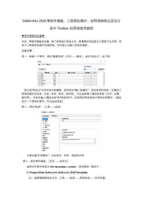
Solidworks 2018零部件模板、工程图标题栏、材料明细表以及设计库中Toolbox的简明使用教程◆零件模板的设置◆目的：零部件模板的设置，除了表明设计信息之外，更重要的用途是与工程图产生关联，有利于工程图的标题栏快速绘制，并杜绝人为输入信息的偏差。

设置步骤：第一，新建一个零件。

调出“摘要信息”（文件——属性），单击“自定义”，如下图：将之前“自定义”中的内容全部删除，然后单击“键入新属性”，添加有用的信息（主要是工程图标题栏的内容，比如：名称、图号、材料等），可以选择每个属性的类型（文字、日期、数字等）。

目前先输入“属性名称”和“类型”即可，后面两栏等具体设计零件时再填写。

（建议设计一个简单的零件，作为直观表现）第二，调出“选项”。

（工具——选项）主要设置“文档属性”，比如单位、字体、表现形式等。

第三、保存零件模板。

（文件——另存为）选择文件保存类型为Part templates (*.prtdot)。

保存路径一般位于：C:\ProgramData\Solidworks\Solidworks 2018\Templates（注：查看模板路径的方法：工具——选项——系统选项——文件位置）可以看到，文件夹中已经有一个自带的名称，可以自己起一个新文件名（我的文件名为My_Part）。

至此，零件模板设置完成。

◆装配体模板的设置◆装配体模板的设置与零件模板类似。

设置步骤：第一，新建一个装配体。

同样，调出“摘要信息”（文件——属性），单击“自定义”。

同样，将之前“自定义”中的内容全部删除，然后单击“键入新属性”，添加有用的信息（主要是装配体工程图标题栏的内容，比如：名称、图号、材料等），每个属性后又类型（文字、日期、数字等）可以选择。

先输入“属性名称”和“类型”即可，后面两栏等具体设计零件时再填写。

建议此标题栏与零件标题栏相同，目的是方便装配体工程图的设置工作量（当然，也可以不同）。

第二，调出“选项”。

Maple Toolbox for Matlab 工具箱的使用向导MapleToolboxforMATLAB操

特征细节：
交互式技术文档环境
• 完整的文档组件 ( 文本、数学、图形、动画等 ), 您可以制作专业水平的、图文并茂的技术文件让您的文件具有可读性和交互性，同时用户可以捕获结果中的知识。并可以利用这个技术文件。 • 直观的二维数学编辑器，让您编写出印刷水准的数学文件。
The Maple™ Toolbox for MATLAB®
The Maple Toolbox for MATLAB includes:
Maple 10 - the most powerful and intuitive tool for solving complex mathematical problems and creating rich, executable technical documents. Maple - MATLAB Connector - a two-way link between Maple and MATLAB, enabling users to define variables in either environment and use them in the other.
jacobian - compute the Jacobian matrix symsum - symbolic sum
Polynomial Manipulation
coeffs collect exp expand factor findsym gcd horner lcm mod - extract all coefficients of a multivariate polynomial - collect coefficients - the exponential function - expand - factor a multivariate polynomial - find symbols - greatest common divisor of polynomials - horner form - least common multiple - computation over the integers modulo m

Matlab Bayes Net Toolbox - 快速操作多维数组说明书

Fast manipulation of multi-dimensional arrays in MatlabKevin P.Murphy**************.edu11September20021IntroductionProbabilistic inference in graphical models with discrete random variables requires performing various oper-ations on multi-dimensional arrays(discrete potentials).This is true whether we use an exact algorithm like junction tree[CDLS99,HD96]or an approximate algorithm like loopy belief propagation[AM00,KFL01]. These operations consist of element-wise multiplication/division of two arrays of potentially diﬀerent sizes, and summation(marginalization)over a subset of the dimensions.This report discusses eﬃcient ways to implement these operations in Matlab,with an emphasis on the implementation used in the Bayes Net Toolbox(BNT).2Running exampleWe will introduce an example to illustrate the problems we want to solve.Consider two arrays(tables), Tbig and Tsmall,where Tbig represents a function over the variables X1,X2,X3,X4and Tsmall represents a function over X1,X3.We will say Tbig’s domain is(1,2,3,4),Tsmall’s domain is(1,3),and the diﬀerence in their domains is(2,4).Let the size of variable X i(i.e.,the number of possible values it can have)be denoted by S i.Here is a straighforward implementation of elementwise multiplication:for i1=1:S1for i2=1:S2for i3=1:S3for i4=1:S4Tbig[i1,i2,i3,i4]=Tbig[i1,i2,i3,i4]*Tsmall[i1,i3];endendendendSimilarly,here is a straightforward implementation of marginalizing the big array onto the small domain: for i1=1:S1for i3=1:S3sum=0;for i2=1:S2for i4=1:S4sum=sum+Tbig[i1,i2,i3,i4];endendTsmall[i1,i3]=sum;endendOf course,these are not general solutions,because we have hard-coded the fact that Tbig is4-dimensional, Tsmall is2-dimensional,and that we are marginalizing over dimensions2and4.The general solution requires mapping vectors of indices(or subscripts)to1dimensional indices(oﬀsets into a1D array),and vice versa. We discuss these auxiliary functions next,before discussing a variety of diﬀerent solutions based on these functions.3Auxiliary functions3.1Converting from multi-dimensional indices to1D indicesIf a d-dimensional array is stored in memory such that the left-most indices toggle fastest(as in Matlab and Fortran—C follows the opposite convention,toggling the right-most indices fastest),then we can compute the1D index from a vector of indices,subs,as follows:ndx=1+(i1-1)+(i2-1)*S1+(i3-1)*S1*S2+...+(id-1)*S1*S2*...*S(d-1) where the vector of indices is subs=(i1,...,i d),and the size of the dimensions are sz=(S1,...,S d). (We only need to add and subtract1if we use1-based indexing,as in Matlab;in C,we would omit this step.)This can be written more concisely asndx=1+sum((subs-1).*[1cumprod(sz(1:end-1))])If we pass the subscripts separately,we can use the built-in Matlab functionndx=sub2ind(sz,i1,i2,...)BNT oﬀers a similar function,except the subscripts are passed as a vector:ndx=subv2ind(sz,subs)The BNT function is vectorized,i.e.,if each row of subs contains a set of subscripts.then ndx will be a vector of1D indices.This can be computed by simple matrix multiplication.For example,ifsubs=[111;211;...222];and sz=[222],then subv2ind(sz,subs)returns[12...8]’,which can be computed usingcp=[1cumprod(siz(1:end-1))]’;ndx=(subs-1)*cp+1;If all dimensions have size2,this is equivalent to converting a binary number to decimal.3.2Converting from1D indices to multi-dimensional indicesWe convert from1D to multi-D by dividing(which is slower).For instance,if subs=(1,3,2)and sz= (4,3,3),then ndx will bendx=1+(1−1)∗1+(3−1)∗4+(2−1)∗4∗3=21To convert back we geti1=1+ (21−1)mod41=1i2=1+ (21−1)mod124=3i3=1+ (21−1)mod3612=2The matlab and BNT functions sub2ind and subv2ind do this.Note:If all dimensions have size2,this is equivalent to converting a decimal to a binary number.3.3Comparing diﬀerent domainsIn our example,Tbig’s domain was(X1,X2,X3,X4)and Tsmall’s domain was(X1,X3).The identity of the variables does not matter;what matters is that for each dimension in Tsmall,we canﬁnd the corresponding/ equivalent dimension in Tbig.This is called a mapping,and can be computed in BNT usingmap=find_equiv_posns(small_domain,big_domain)(In R,this function is called match.In Phrog[Phr],this is called an RvMapping.)If smalldom=(1,3) and bigdom=(1,2,3,4),then map=(1,3);if smalldom=(8,2)and bigdom=(2,7,4,8),then map= (4,1);etc.4Naive methodGiven the above auxiliary functions,we can implement multiplication as follows:map=find_equiv_posns(Tsmall.domain,Tbig.domain);for ibig=1:prod(Tbig.sizes)subs_big=ind2subv(Tbig.sizes,ibig);subs_small=subs_big(map);ismall=subv2ind(Tsmall.sizes,subs_small);Tbig.T(ibig)=Tbig.T(ibig)*Tsmall.T(ismall);end(Note that this involves a single write to Tbig in sequential order,but multiple reads from Tsmall in a random order;this can aﬀect cache performance.)Marginalization can be implemented as follows(other methods are possible,as we will see below). Tsmall.T=zeros(Tsmall.sizes);map=find_equiv_posns(Tsmall.domain,Tbig.domain);for ibig=1:prod(Tbig.sizes)subs_big=ind2subv(Tbig.sizes,ibig);subs_small=subs_big(map);ismall=subv2ind(Tsmall.sizes,subs_small);Tsmall.T(ismall)=Tsmall.T(ismall)+Tbig.T(ibig);end(Note that this involves multiple writes to Tsmall in a random order,but a single read of each element of Tbig in sequential order;this can aﬀect cache performance.)The problem is that calling ind2subv and subv2ind inside the inner loop is very slow,so we now seek faster methods.Row ndx 1111211112112211112121211221222111122112121222121122212212222222look up the indices,we need to convert map and big-sizes,both of which are lists of positive(small)integers, into integers.This could be done with a hash function.This makes it possible to hide the presence of the cache inside an object(call it a TableEngine)which can multiply/marginalize(pairs of)tables,e.g., function Tbig=multiply(TableEngine,Tsmall,Tbig)map=find_equiv_posns(Tsmall.domain,Tbig.domain);cache_entry_num=hash_fn(map,Tbig.sizes);ndx=TableEngine.ndx_cache{cache_entry_num};Tbig.T(:)=Tbig.T(:).*Tsmall.T(ndx);One big problem with Matlab is that Tbig will be passed by value,since it is modiﬁed within the function, and then copied back to the callee.This could be avoided if functions could be inlined,or if pass by reference were supported,but this is not possible with the current version of Matlab.Another problem is that computing the hash function is slow in Matlab,so what I currently do in BNT is explicitely store the cache-entry-num for every pair of potentials that will be multiplied(i.e.,for every pair of neighboring cliques in the jtree).Also,for every potential,I store the cache-entry-num for every domain onto which the potential may be marginalized(this corresponds to all families and singletons in the bnet). This allows me to quickly retrieve the relevant cache entry,but unfortunately requires the inference engine to be aware of the presence of the cache.That is,the current code(inside jtree-ndx-inf-engine/collect-evidence) looks more like the following:ndx=B_NDX_CACHE{engine.mult_cl_by_sep_ndx_id(p,n)};ndx=double(ndx)+1;Tsmall=Tsmall(ndx);Tbig(:)=Tbig(:).*Tsmall(:);where mult-cl-by-sep-ndx-id(p,n)is the cache entry number for multiplying clique p by separator n.By implementing a TableEngine with a hash function,we could hide the presence of the cache,and simplify the code.Furthermore,instead of having jtree-inf and jtree-ndx-inf,we would have a single class,jtree-inf,which could use diﬀerent implementations of the TableEngine object,e.g.,with or without cacheing.Indeed,any code that manipulates tables(e.g.,loopy)would be able to use diﬀerent implementations of TableEngine. We will now discuss other possible implementations of the TableEngine,which use diﬀerent kinds of indices, or even no indices at all.7Reducing the size of the indices:ndxSDWe can reduce the space requirements for storing the indices from B to S+D,where S=prod(sz(Tsmall.domain)) and D=prod(sz(diﬀ-domain)).To explain how this works,let usﬁrst rewrite the marginalization code,so that we write to each element of Tsmall once in sequential order,but do multiple random reads from Tbig (the opposite of before).small_map=find_equiv_posns(Tsmall.domain,Tbig.domain);diff=setdiff(Tbig.domain,Tsmall.domain);diff_map=find_equiv_posns(diff,Tbig.domain);diff_sz=Tbig.sizes(diff_map);for ismall=1:prod(Tsmall.sizes)subs_small=ind2subv(Tsmall.sizes,ismall);subs_big=zeros(1,length(Tbig.domain));sum=0;for jdiff=1:prod(diff_sz)subs_diff=ind2subv(diff_sz,idff);subs_big(small_map)=subs_small;subs_big(subs_diff)=subs_diff;ibig=subv2ind(Tbig.sizes,subs_big);sum=sum+Tbig.T(ibig);endTsmall.T(ismall)=sum;endNow suppose we have a function that computes ibig given ismall and jdiﬀ,call it index(ismall,jdiﬀ). Then we can rewrite the above as follows:for ismall=1:prod(Tsmall.sizes)sum=0;for jdiff=1:prod(diff_sz)sum=sum+Tbig.T(index(ismall,jdiff));endTsmall.T(ismall)=sum;endSimilarly,we can implement multiplication by doing a single write to Tbig in a random order,and multiple sequential reads from Tsmall(the opposite of before).for ismall=1:prod(Tsmall.sizes)for jdiff=1:prod(diff_sz)ibig=index(ismall,jdiff);Tbig.T(ibig)=Tbig.T(ibig)*Tsmall.T(ismall);endend7.1Computing the indicesWe now explain how to compute the index(what[Phr]calls a FactorMapping)using our running example.1 Referring to Table1,we see that entries1,3,9,11of Tbig map to Tsmall(1),entries2,4,10,12map to2, entries5,7,13,15map to3,and entries6,8,14,16map to4.Instead of keeping the whole ndx,it is suﬃcient to keep two tables:one that keeps theﬁrst value of each group,call it start(in this case[1,2,5,6])and one that keeps the oﬀset from the start within each group(in this case[0,2,8,10]).(In BNT,start is called small-ndx and oﬀset is called diﬀ-ndx.)Then we haveindex(ismall,jdiff)=start(ismall)+offset(jdiff)We can compute the start positions by noticing that,in this example,we just increment X1and X3, keeping the remaining dimensions(the diﬀdomain)constantly clamped to1;this can be implemented by setting the eﬀective size of the diﬀerence dimensions to1(so they only have1possible value).diff_domain=mysetdiff(Tbig.domain,Tsmall.domain);diff_sizes=Tbig.sizes(map);map=find_equiv_posns(diff_domain,Tbig.domain);sz=Tbig.sizes;sz(map)=1;%sz(diff)is1,sz(small)is normalsubs=ind2subv(sz,1:prod(Tsmall.sizes));start=subv2ind(Tbig.sizes,subs);Similarly,we can compute the oﬀsets by incrementing X2and X4,keeping X1and X3ﬁxed.map=find_equiv_posns(Tsmall.domain,Tbig.domain);sz=Tbig.sizes;sz(map)=1;%sz(small)is1,sz(diff)is normalsubs=ind2subv(sz,1:prod(diff_sz));offset=subv2ind(Tbig.sizes,subs)-1;7.2Avoiding for-loopsGiven start and oﬀset,we can implement multiplication and marginalization using two for-loops,as shown above.This is fast in C,but slow in Matlab.For small problems,it is possible to vectorize both operations,as follows.First we create a matrix of indices,ndx2,from start and oﬀset,as follows:ndx2=repmat(start(:),1,prod(diff_sizes))+repmat(offset(:)’,prod(Tsmall.sizes),1);In our example,this produces1111222255556666 +02810028100281002810 =13911241012571315681416Row 1contains the locations in Tbig which should be summed together and stored in Tsmall(1),etc.Hence we can writeTsmall.T =sum(Tbig.T(ndx2),2);For multiplication,each element of Tsmall gets mapped to many elements of Tbig,hence Tbig.T(ndx2(:))=Tbig.T(ndx2(:)).*repmat(Tsmall.T(:),prod(diff_sz),1);8Eliminating for-loops and indicesWe can eliminate the need for for-loops and indices as follows.We make Tsmall the same size as Tbig by replicating entries where necessary,and then just doing an element-wise multiplication:temp =extend_domain(Tsmall.T,Tsmall.domain,Tsmall.sizes,Tbig.domain,Tbig.sizes);Tbig.T =Tbig.T .*temp;Let us explain extend-domain using our standard example.First we reshape Tsmall to make it have size [2121],so it has the same number of dimensions as Tbig.(This involves no real work.)map =find_equiv_posns(smalldom,bigdom);sz =ones(1,length(bigdom));sz(map)=small_sizes;Tsmall =reshape(Tsmall,sz);Now we replicate Tsmall along dimensions 2and 4,to make it the same size as big-sizes (we assume the variables have a standardized order,so there is no need to permute dimensions).sz =big_sizes;sz(map)=1;Tsmall =repmat(Tsmall,sz(:)’);Now we are ready to multiply:Tbig .*Tsmall .For small problems,this is faster,at least in Matlab,but in C,it would be faster to avoid copying memory.Doug Schwarz wrote a genops class using C that can avoid the repmat above.See /∼schwarz/genops.html (unfortunately no longer available online).For marginalization,we can simply call Matlab’s built-in sum command on each dimension,and then squeeze the result,to get rid of dimensions that have been reduced to size 1(we must remember to put back any dimensions that were originally size 1,by reshaping).Method Section ndx MargTsmall Tbig vecmulti rnd rd sgl seq wr yesmulti seq rd sgl rnd wr norepmat sgl rnd wr yesrepmat sgl seq wr yes[KFL01] F.Kschischang,B.Frey,and H-A.Loeliger.Factor graphs and the sum-product algorithm.IEEE Trans Info.Theory,February2001.[Phr]Phrog:Stanford’s C++Bayes Net package./frog/mappings.html.。

robotic toolbox 使用说明

Robotic Toolbox工具箱使用方法1．坐标变换利用MATLAB中Robotics Toolbox工具箱中的transl、rotx、roty和rotz可以实现用齐次变换矩阵表示平移变换和旋转变换。

下面举例来说明：A 机器人在x轴方向平移了0.5米，那么我们可以用下面的方法来求取平移变换后的齐次矩阵：>> transl(0.5,0,0)ans =1.0000 0 0 0.50000 1.0000 0 00 0 1.0000 00 0 0 1.0000B 机器人绕x轴旋转45度，那么可以用rotx来求取旋转后的齐次矩阵：>> rotx(pi/4)ans =1.0000 0 0 00 0.7071 -0.7071 00 0.7071 0.7071 00 0 0 1.0000C 机器人绕y轴旋转90度，那么可以用roty来求取旋转后的齐次矩阵：>> roty(pi/2)ans =0.0000 0 1.0000 00 1.0000 0 0-1.0000 0 0.0000 00 0 0 1.0000D 机器人绕z轴旋转-90度，那么可以用rotz来求取旋转后的齐次矩阵：>> rotz(-pi/2)ans =0.0000 1.0000 0 0-1.0000 0.0000 0 00 0 1.0000 00 0 0 1.0000当然，如果有多次旋转和平移变换，我们只需要多次调用函数在组合就可以了。

另外，可以和我们学习的平移矩阵和旋转矩阵做个对比，相信是一致的。

2. 构建机器人对象要建立机器人对象，首先我们要了解D-H参数，之后我们可以利用Robotics Toolbox工具箱中的link和robot函数来建立机器人对象。

TOOLBOX培训

— Parts Info — Fault Isolation
27
查询功能2
System — Synoptics
根据飞机信息搜索机型选择
飞机选择
点击Synoptics 按钮
28
查询功能2
System — Synoptics
选择一个或多个飞机系统
选择Get Result
选择一个Synoptic
7
一般功能介绍
MyBoeingFleet主页：
Maintenance Performance Toolbox
8
一般功能介绍
Maintenance Performance Toolbox主页1：My Inbox
Structured Data in SGML (manual-oriented) PDF
36
查询功能2
System — Line Replaceable Unit
选择机型、飞机后点击Line Replaceable Unit按钮
37
查询功能2
System — Line Replaceable Unit
可以根据Select One or More Systems选择一个或多个系统，或者Search by L LRU List按钮。
34
查询功能2
System — Synoptics
在LRU List内拖动鼠标，相关的LRU项目会与右侧图表内相关的框图同时变红。
35
查询功能2
System — Synoptics
如果鼠标放在LRU框图上，屏幕显示有“Goes to”字样，则代表还有子框图，点击后进入子框图屏幕。
System — Fault Isolation

MATLAB中的优化工具箱使用指南

MATLAB中的优化工具箱使用指南导言MATLAB（Matrix Laboratory）是一种高级计算机编程语言和环境，主要用于算法开发、数据分析和可视化。

作为一款强大的科学计算工具，它提供了众多的工具箱，其中之一就是优化工具箱。

本文将为大家介绍如何使用MATLAB中的优化工具箱，以便更好地应用于各种优化问题的求解。

第一节优化问题概述优化问题是指在满足一定约束条件下，寻找一个或一组使目标函数最优化的变量取值。

在现实生活中，我们常常需要优化问题来解决实际的工程、经济等领域中的复杂问题。

例如，运输问题、资源分配问题、最大化收益问题等都可以归结为优化问题。

在MATLAB中，我们可以利用优化工具箱中的函数和算法来解决这些问题。

第二节优化工具箱基本功能优化工具箱为我们提供了一系列功能强大的函数，用于求解不同类型的优化问题。

其中最常用的函数包括：fminbnd、fmincon、fminsearch、linprog等。

下面分别介绍这些函数的基本用法。

1. fminbnd：用于求解一维无约束优化问题，即在一个区间内寻找一个函数的最小值。

例如，我们要求解函数f(x) = x^2在区间[0, 1]上的最小值，可以使用fminbnd函数。

2. fmincon：用于求解多维有约束优化问题。

它需要输入目标函数、约束条件以及初始解等参数，并且可以自定义优化算法。

例如，我们要求解函数f(x) = x1^2 + x2^2在满足约束条件x1 + x2 = 1时的最小值，可以使用fmincon函数。

3. fminsearch：用于求解多维无约束优化问题。

它需要输入目标函数和初始解等参数，并且可以选择不同的优化算法。

例如，我们要求解函数f(x) = x1^2 + x2^2的最小值，可以使用fminsearch函数。

4. linprog：用于线性规划问题的求解，即在一组线性约束条件下求解目标函数的最小值或最大值。

它需要输入目标函数、约束条件以及目标类型（最小化或最大化）等参数，可以返回最优解以及最优目标函数值。

AIX下的媒体播放器xmms的安装与使用

AIX下的媒体播放器xmms的安装与使用Windows的用户可能会比较熟悉Winamp播放软件，很多人都用它来听MP3。

那么在AIX上能不能播放MP3呢？回答是肯定的。

但是IBM提供的AIX操作系统中并没有提供多媒体格式文件的播放器，例如MP3、MIDI等格式的播放器。

然而UNIX的开放性使得不少Linux下的开源（OpenSource）软件经过重新编译以后可以在AIX下运行，因此，我们可以在AIX的CDE环境下使用一款早已在Linux下风靡一时的多媒体播放器xmms。

xmms全称X MultiMedia System，它支持MP3、Wav、Midi、Vqf等常见的音频格式，同时具有丰富的音频控制（EQ）、视频感观插件。

一、xmms的安装。

xmms在AIX下的安装要比一般的软件稍微复杂一些。

因为xmms的运行依赖比较多的预先装好的运行库，只有按照正确的顺序全部安装好了运行库，xmms才能够正确的运行。

首先我们需要从Linux Toolbox for AIX的光盘上找到xmms的文件包，或者您可以从IBM的Linux Toolbox for AIX的网站（/servers/aix/products/aixos/linux/altlic.html）下载xmms软件。

IBM提供的xmms是rpm格式的1.2.7版本的软件――xmms-1.2.7-1.aix4.3.ppc.rpm。

这款软件可以安装在AIX V4.3.3 或者 AIX 5L上。

但是安装xmms之前，我们还需要安装GIMP ToolKit。

GIMP ToolKit 是一个库文件，是在X Window环境之下创建GUI（图形用户界面）的必备库。

幸运的是，IBM在Linux Toolbox for AIX中也提供了 GIMP ToolKit――gtkplus-1.2.10-3.aix4.3.ppc.rpm，同样是rpm包的。

在安装GIMP ToolKit之前，还必须安装一个很多函数都要调用的标准库glib，同样可以从IBM Linux Toolbox网站下载到。

1、下载文档前请自行甄别文档内容的完整性，平台不提供额外的编辑、内容补充、找答案等附加服务。
2、"仅部分预览"的文档,不可在线预览部分如存在完整性等问题,可反馈申请退款(可完整预览的文档不适用该条件!)。
3、如文档侵犯您的权益，请联系客服反馈,我们会尽快为您处理(人工客服工作时间：9:00-18:30)。

Multimedia Toolbox Guide1Shannon WhitmoreEric ShafferRuth Aydt

Pablo Research GroupDepartment of Computer ScienceUniversity of IllinoisUrbana, Illinois 61801

http://www-pablo.cs.uiuc.eduJanuary 30, 1998

1 Supported in part by DARPA contracts DABT63-96-C-0027, DABT63-96-C-0161 and by the National

Science Foundation under grants IRI 92-12976 and NSF CDA94-01124.Contents1Introduction...........................................................................................................................................61.1Multimedia Annotation Rationale...................................................................................................61.2Virtue..............................................................................................................................................61.3Terminology....................................................................................................................................81.4System Overview............................................................................................................................91.5Major Functionality......................................................................................................................101.5.1Annotation Record and Playback..............................................................................................111.5.2Real-time Collaboration............................................................................................................111.5.3Announcement System.............................................................................................................111.6Roadmap.......................................................................................................................................11

2Getting Started – A Tutorial..............................................................................................................122.1Setup.............................................................................................................................................122.1.1Verify Regular Vic and Vat......................................................................................................122.1.2Annotation Directory................................................................................................................122.1.3.mmrc Resource File.................................................................................................................132.1.4vic and vat Command Line Options.........................................................................................152.1.5Environment Variables.............................................................................................................152.1.6Log Files...................................................................................................................................152.2Running the Test Client................................................................................................................162.2.1Start the Servers........................................................................................................................162.2.2Start test_cli..............................................................................................................................172.2.3Start the Local Streams.............................................................................................................182.2.4Set Audio and Video Source ID................................................................................................192.2.5Record an Annotation...............................................................................................................192.2.6Replay an Annotation...............................................................................................................202.2.7Freeze/Unfreeze a Video Stream..............................................................................................212.2.8Kill the Servers/Quit the Client.................................................................................................212.2.9Cleanup.....................................................................................................................................21

3Multimedia Toolbox...........................................................................................................................233.1Annotation Server.........................................................................................................................233.1.1New Annotation........................................................................................................................243.1.2Synchronize Audio/Video Annotations....................................................................................243.1.3Replay Annotations...................................................................................................................243.2Record Servers..............................................................................................................................253.2.1Start Record..............................................................................................................................263.2.2Stop Record..............................................................................................................................263.3Playback Servers...........................................................................................................................273.3.1Playback Annotation.................................................................................................................273.4Audio/Video Servers.....................................................................................................................283.4.1Real-time Collaboration............................................................................................................293.4.2Announcement System.............................................................................................................293.5Running the Servers on Different Hosts.......................................................................................31