Bayesian Forecasting using Stochastic Search Variable Selection in a VAR Subject to Breaks
Bayesian Hypothesis Testing and Bayes Factors
The General Form for Bayes Factors
Suppose that we observe data X and with to test two competing models—M1 and M2, relating these data to two different sets of parameters, θ1 and θ2. We would like to know which of the following likelihood specifications is better: M1: f1(x | θ1) and M2: f2(x | θ1) Obviously, we would need prior distributions for the θ1 and θ2 and prior probabilities for M1 and M2 The posterior odds ratio in favor of M1 over M2 is:
Bayes Factors
Notes taken from Gill (2002)
Bayes Factors are the dominant method of Bayesian model testing. They are the Bayesian analogues of likelihood ratio tests. The basic intuition is that prior and posterior information are combined in a ratio that provides evidence in favor of one model specification verses another. Bayes Factors are very flexible, allowing multiple hypotheses to be compared simultaneously and nested models are not required in order to make comparisons -it goes without saying that compared models should obviously have the same dependent variable.
统计学、概率论和数理统计的区别和联系

统计学、概率论和数理统计的区别和联系今天我们就来说说统计学、概率论和数理统计为什么要说他们呢,因为这⼏个字眼⼤家肯定是已经⽆数次地碰到过了,但他们究竟代表了什么,以及他们之间的区别与联系,相信⼤家平时肯定是没怎么关注过,⽽是更多的混为⼀谈。
然⽽今天,随着⼤数据与数据科学的热⽕朝天,这⼏个词重新被⼤家给予了⾼度关注,特别是统计学。
原因也很⾃然:分析思维是数据科学的核⼼思维⽅式,⽽分析思维就是关于计算与统计的思维。
统计思维⽣长的⼟壤就是概率论和数理统计。
1、统计学⾸先说说统计学,关于这个词其实是个历史遗留问题。
因为从统计学的发展历史来看,最早的统计学和国家经济学有密切的关系。
统计学的英⽂是“statistic”,其实它是源于意⼤利⽂的“stato”,意思是“国家”、“情况”,也就是后来英语⾥的state(国家),在⼗七、⼗⼋世纪,统计学很多时候都是以经济学的姿态出现的。
根据维基百科:By the 18th century, the term 'statistics' designated the systematic collection of demographic and economic data by states. For at least two millennia, thesedata were mainly tabulations of human and material resources that might betaxed or put to military use.统计学最开始来源于经济学和政治学。
17世纪的经济学家William Petty和他的《政治算术》⼀书揭开了统计学的起源(维基百科):The birth of statistics is often dated to 1662, when John Graunt, along with William Petty, developed early human statistical and census methods that provided a framework for modern demography. He produced the first life table, giving probabilities of survival to each age. Hisbook Natural and Political Observations Made upon the Bills of Mortality usedanalysis of the mortality rolls to make the first statistically basedestimation of the population of London.所以从⼀开始,统计学就跟经济学、政治学密不可分的。
Bayesian Inference
p(black) = 18/38 = 0.473
p(red) = 18/38 = 0.473
p(color )
What is a conditional probability?
p(black|col1) = 6/12 = 0.5
p(color | col1)
p(black|col2) = 8/12 = 0.666
p(x)
Bayesian Roulette
• We’re interested in which column will win. • p(column) is our prior. • We learn color=black.
Bayesian Roulette
• • • • We’re interested in which column will win. p(column) is our prior. We learn color=black. What is p(color=black|column)?
What do you need to know to use it?
• You need to be able to express your prior beliefs about x as a probability distribution, p (x ) • You must able to relate your new evidence to your variable of interest in terms of it’s likelihood, p(y|x) • You must be able to multiply.
p(black|col1) = 6/12 = 0.5 p(black|col2) = 8/12 = 0.666 p(black|col3) = 4/12 = 0.333 p(black|zeros) = 0/2 = 0
Bayesian representation of stochastic processes under learning De finetti revisited
Matthew O. Jackson Ehud Kalai Revised: May 6, 1998
Abstract
Rann Smorodinsky
1
weakened to an asymptotic mixing condition, and with his conclusion of a decomposition into iid component distributions weakened to components that are learnable and su cient for prediction.
R R R
0 0
1 For example, Nyarko 1996 argues that it is important for learning results in incomplete information games to be robust to equivalent reformulations of type spaces. He discusses examples which are not robust to such reformulations. In the language of this paper the reformulations are di erent representations of the process associated with the same game and strategies.
A probability distribution governing the evolution of a stochastic process has in nitely many Bayesian representations of the form R = d . Among these, a natural representation is one whose components 's are `learnable' one can approximate by conditioning on observation of the process and `su cient for prediction' 's predictions are not aided by conditioning on observation of the process. We show the existence and uniqueness of such a representation under a suitable asymptotic mixing condition on the process. This representation can be obtained by conditioning on the tail- eld of the process, and any learnable representation that is su cient for prediction is asymptotically like the tail- eld representation. This result is related to the celebrated de Finetti theorem, but with exchangeability
AB实验的高端玩法系列1-AB实验人群定向个体效果差异HTEUpliftModel论文gi。。。

AB实验的⾼端玩法系列1-AB实验⼈群定向个体效果差异HTEUpliftModel论⽂gi。
⼀直以来机器学习希望解决的⼀个问题就是'what if',也就是决策指导:如果我给⽤户发优惠券⽤户会留下来么?如果患者服了这个药⾎压会降低么?如果APP增加这个功能会增加⽤户的使⽤时长么?如果实施这个货币政策对有效提振经济么?这类问题之所以难以解决是因为ground truth在现实中是观测不到的,⼀个已经服了药的患者⾎压降低但我们⽆从知道在同⼀时刻如果他没有服药⾎压是不是也会降低。
这个时候做分析的同学应该会说我们做AB实验!我们估计整体差异,显著就是有效,不显著就是⽆效。
但我们能做的只有这些么?当然不是!因为每个个体都是不同的!整体⽆效不意味着局部群体⽆效!如果只有5%的⽤户对发优惠券敏感,我们能只触达这些⽤户么?或者不同⽤户对优惠券敏感的阈值不同,如何通过调整优惠券的阈值吸引更多的⽤户?如果降压药只对有特殊症状的患者有效,我们该如何找到这些患者?APP的新功能部分⽤户不喜欢,部分⽤户很喜欢,我能通过⽐较这些⽤户的差异找到改进这个新功能的⽅向么?以下⽅法从不同的⾓度尝试解决这个问题,但基本思路是⼀致的:我们⽆法观测到每个⽤户的treatment effect,但我们可以找到⼀群相似⽤户来估计实验对他们的影响。
我会在之后的博客中,从CasualTree的第⼆篇Recursive partitioning for heterogeneous causal effects开始梳理下述⽅法中的异同。
整个领域还在发展中,⼏个开源代码都刚release不久,所以这个博客也会持续更新。
如果⼤家看到好的⽂章和⼯程实现也欢迎在下⾯评论~Uplift Modelling/Causal Tree1. Nicholas J Radcliffe and Patrick D Surry. Real-world uplift modelling with significance based uplift trees. White Paper TR-2011-1,Stochastic Solutions, 2011.2. Rzepakowski, P. and Jaroszewicz, S., 2012. Decision trees for uplift modeling with single and multiple treatments. Knowledge andInformation Systems, 32(2), pp.303-327.3. Yan Zhao, Xiao Fang, and David Simchi-Levi. Uplift modeling with multiple treatments and general response types. Proceedings ofthe 2017 SIAM International Conference on Data Mining, SIAM, 2017.4. Athey, S., and Imbens, G. W. 2015. Machine learning methods forestimating heterogeneous causal effects. stat 1050(5)5. Athey, S., and Imbens, G. 2016. Recursive partitioning for heterogeneous causal effects. Proceedings of the National Academy ofSciences.6. C. Tran and E. Zheleva, “Learning triggers for heterogeneous treatment effects,” in Proceedings of the AAAI Conference on ArtificialIntelligence, 2019Forest Based Estimators1. Wager, S. & Athey, S. (2018). Estimation and inference of heterogeneous treatment effects using random forests. Journal of theAmerican Statistical Association .2. M. Oprescu, V. Syrgkanis and Z. S. Wu. Orthogonal Random Forest for Causal Inference. Proceedings of the 36th InternationalConference on Machine Learning (ICML), 2019Double Machine Learning1. V. Chernozhukov, D. Chetverikov, M. Demirer, E. Duflo, C. Hansen, and a. W. Newey. Double Machine Learning for Treatment andCausal Parameters. ArXiv e-prints2. V. Chernozhukov, M. Goldman, V. Semenova, and M. Taddy. Orthogonal Machine Learning for Demand Estimation: HighDimensional Causal Inference in Dynamic Panels. ArXiv e-prints, December 2017.3. V. Chernozhukov, D. Nekipelov, V. Semenova, and V. Syrgkanis. Two-Stage Estimation with a High-Dimensional Second Stage.2018.4. X. Nie and S. Wager. Quasi-Oracle Estimation of Heterogeneous Treatment Effects. arXiv preprint arXiv:1712.04912, 2017.5. D. Foster and V. Syrgkanis. Orthogonal Statistical Learning. arXiv preprint arXiv:1901.09036, 2019Meta Learner1. C. Manahan, 2005. A proportional hazards approach to campaign list selection. In SAS User Group International (SUGI) 30Proceedings.2. Green DP, Kern HL (2012) Modeling heteroge-neous treatment effects in survey experiments with Bayesian additive regression trees.Public OpinionQuarterly 76(3):491–511.3. Sören R. Künzel, Jasjeet S. Sekhon, Peter J. Bickel, and Bin Yu. Metalearners for estimating heterogeneous treatment effects usingmachine learning. Proceedings of the National Academy of Sciences, 2019.Deep Learning1. Fredrik D. Johansson, U. Shalit, D. Sontag.ICML (2016). Learning Representations for Counterfactual Inference2. Shalit, U., Johansson, F. D., & Sontag, D. ICML (2017). Estimating individual treatment effect: generalization bounds and algorithms.Proceedings of the 34th International Conference on Machine Learning3. Christos Louizos, U. Shalit, J. Mooij, D. Sontag, R. Zemel, M. Welling.NIPS (2017). Causal Effect Inference with Deep Latent-VariableModels4. Alaa, A. M., Weisz, M., & van der Schaar, M. (2017). Deep Counterfactual Networks with Propensity-Dropout5. Shi, C., Blei, D. M., & Veitch, V. NeurIPS (2019). Adapting Neural Networks for the Estimation of Treatment EffectsUber专场最早就是uber的博客在茫茫paper的海洋中帮我找到了⽅向,如今听说它们AI LAB要解散了有些伤感,作为HTE最多star的开源⽅,它们值得拥有⼀个part1. Shuyang Du, James Lee, Farzin Ghaffarizadeh, 2017, Improve User Retention with Causal Learning2. Zhenyu Zhao, Totte Harinen, 2020, Uplift Modeling for Multiple Treatments with Cost3. Will Y. Zou, Smitha Shyam, Michael Mui, Mingshi Wang, 2020, Learning Continuous Treatment Policy and Bipartite Embeddings forMatching with Heterogeneous Causal EffectsOptimization4. Will Y. Zou,Shuyang Du,James Lee,Jan Pedersen, 2020, Heterogeneous Causal Learning for Effectiveness Optimizationin User Marketing想看更多因果推理AB实验相关paper的⼩伙伴看过来持续更新中 ~。
基于贝叶斯神经网络方法短期负荷预测指南

基于贝叶斯神经网络方法短期负荷预测指南短期负荷预测在电力系统运行中起着至关重要的作用。
正确的负荷预测可以帮助电力公司合理调度发电机组,优化电力供需平衡,提高电力系统的可靠性和经济性。
贝叶斯神经网络(Bayesian Neural Network,BNN)作为一种强大的建模工具,已经在负荷预测领域取得了很好的效果。
本文将介绍基于BNN方法进行短期负荷预测的指南。
首先,我们需要准备历史负荷数据作为训练样本。
这些历史负荷数据通常包括负荷的时间序列和对应的日期时间信息。
为了提高预测模型的准确性,我们可以考虑使用一些相关的影响因素作为特征变量,例如天气数据、季节性因素等。
接下来,我们需要选择一个合适的BNN模型结构。
BNN是一种基于神经网络的概率图模型,可以有效处理不确定性问题。
常见的BNN模型包括Bayesian Feedforward Neural Network(BFNN)、Bayesian Recurrent Neural Network(BRNN)等。
根据实际需求,选择一个适合的模型。
在训练BNN模型之前,我们需要进行数据预处理。
常见的预处理方法包括标准化、归一化等,以提高数据的可比性和模型的训练效果。
接着,我们可以使用一些常见的优化算法训练BNN模型,例如随机梯度下降(Stochastic Gradient Descent,SGD)、Adam等。
在进行优化算法调参时,可以使用交叉验证的方法选择最优的参数配置。
训练好BNN模型后,我们可以进行负荷预测。
预测的输入是未来一段时间的特征变量,输出是对应时间段的负荷预测结果。
预测结果可以是点预测,也可以是概率分布预测。
最后,我们需要评估负荷预测的准确性。
常见的评估指标包括均方根误差(Root Mean Square Error,RMSE)、平均绝对误差(MeanAbsolute Error,MAE)等。
通过对预测准确性的评估,可以判断BNN模型的负荷预测效果,并进行相应的改进。
贝叶斯矢量自回归模型与随机波动率和时变参数的分析软件说明书
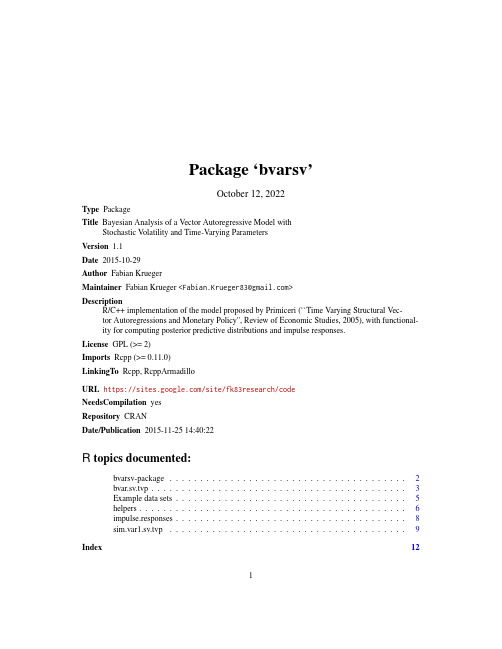
Package‘bvarsv’October12,2022Type PackageTitle Bayesian Analysis of a Vector Autoregressive Model withStochastic V olatility and Time-Varying ParametersVersion1.1Date2015-10-29Author Fabian KruegerMaintainer Fabian Krueger<**************************>DescriptionR/C++implementation of the model proposed by Primiceri(``Time Varying Structural Vec-tor Autoregressions and Monetary Policy'',Review of Economic Studies,2005),with functional-ity for computing posterior predictive distributions and impulse responses.License GPL(>=2)Imports Rcpp(>=0.11.0)LinkingTo Rcpp,RcppArmadilloURL https:///site/fk83research/codeNeedsCompilation yesRepository CRANDate/Publication2015-11-2514:40:22R topics documented:bvarsv-package (2)p (3)Example data sets (5)helpers (6)impulse.responses (8)p (9)Index1212bvarsv-packagebvarsv-package Bayesian Analysis of a Vector Autoregressive Model with StochasticVolatility and Time-Varying ParametersDescriptionR/C++implementation of the Primiceri(2005)model,which allows for both stochastic volatility and time-varying regression parameters.The package contains functions for computing posterior predictive distributions and impulse responses from the model,based on an input data set.DetailsPackage:bvarsvType:PackageVersion: 1.0Date:2014-08-14License:GPL(>=2)URL:https:///site/fk83research/codeAuthor(s)Fabian Krueger<**************************>,based on Matlab code by Dimitris Korobilis(see Koop and Korobilis,2010).ReferencesThe code incorporates the recent corrigendum by Del Negro and Primiceri(2015),which points to an error in the original MCMC algorithm of Primiceri(2005).Del Negro,M.and Primicerio,G.E.(2015).‘Time Varying Structural Vector Autoregressions and Monetary Policy:A Corrigendum’,Review of Economic Studies82,1342-1345.Koop,G.and D.Korobilis(2010):‘Bayesian Multivariate Time Series Methods for Empirical Macroeconomics’,Foundations and Trends in Econometrics3,267-358.Accompanying Matlab code available at https:///site/dimitriskorobilis/matlab.Primiceri,G.E.(2005):‘Time Varying Structural Vector Autoregressions and Monetary Policy’, Review of Economic Studies72,821-852.Examples##Not run:#Load US macro datadata(usmacro)#Estimate trivariate model using Primiceri s prior choices(default settings)set.seed(5813)bv<p(usmacro)##End(Not run)p Bayesian Analysis of a Vector Autoregressive Model with StochasticVolatility and Time-Varying ParametersDescriptionBayesian estimation of theflexible V AR model by Primiceri(2005)which allows for both stochasticvolatility and time drift in the model parameters.Usagep(Y,p=1,tau=40,nf=10,pdrift=TRUE,nrep=50000,nburn=5000,thinfac=10,itprint=10000,save.parameters=TRUE,k_B=4,k_A=4,k_sig=1,k_Q=0.01,k_S=0.1,k_W=0.01,pQ=NULL,pW=NULL,pS=NULL)ArgumentsY Matrix of data,where rows represent time and columns are different variables.Y must have at least two columns.p Lag length,greater or equal than1(the default)tau Length of the training sample used for determining prior parameters via leastsquares(LS).That is,data in Y[1:tau,]are used for estimating prior parame-ters via LS;formal Bayesian analysis is then performed for data in Y[(tau+1):nrow(Y),].nf Number of future time periods for which forecasts are computed(integer,1orgreater,defaults to10).pdrift Dummy,indicates whether or not to account for parameter drift when simulatingforecasts(defaults to TRUE).nrep Number of MCMC draws excluding burn-in(defaults to50000)nburn Number of MCMC draws used to initialize the sampler(defaults to5000).Thesedraws do not enter the computation of posterior moments,forecasts etc.thinfac Thinning factor for MCMC output.Defaults to10,which means that the fore-cast sequences(fc.mdraws,fc.vdraws,fc.ydraws,see below)contain onlyevery tenth draw of the original sequence.Set thinfac to one to obtain the fullMCMC sequence.itprint Print every itprint-th iteration.Defaults to10000.Set to very large value toomit printing altogether.save.parametersIf set to TRUE,parameter draws are saved in lists(these can be very large).De-faults to TRUE.k_B,k_A,k_sig,k_Q,k_W,k_S,pQ,pW,pSQuantities which enter the prior distributions,see the links below for details.Defaults to the exact values used in the original article by Primiceri.ValueBeta.postmean Posterior means of coefficients.This is an array of dimension[M,Mp+1,T],where T denotes the number of time periods(=number of rows of Y),and Mdenotes the number of system variables(=number of columns of Y).The sub-matrix[,,t]represents the coefficient matrix at time t.The intercept vector isstacked in thefirst column;the p coefficient matrices of dimension[M,M]areplaced next to it.H.postmean Posterior means of error term covariance matrices.This is an array of dimension[M,M,T].The submatrix[,,t]represents the covariance matrix at time t.Q.postmean,S.postmean,W.postmeanPosterior means of various covariance matrices.fc.mdraws Draws for the forecast mean vector at various horizons(three-dimensional array,where thefirst dimension corresponds to system variables,the second to forecasthorizons,and the third to MCMC draws).Note:The third dimension will beequal to nrep/thinfac,apart from possible rounding issues.fc.vdraws Draws for the forecast covariance matrix.Design similar to fc.mdraws,ex-cept that thefirst array dimension contains the lower-diagonal elements of theforecast covariance matrix.fc.ydraws Simulated future observations.Design analogous to fc.mdraws.Beta.draws,H.drawsMatrices of parameter draws,can be used for computing impulse responses lateron(see impulse.responses),and accessed via the helper function parameter.draws.These outputs are generated only if save.parameters has been set to TRUE.Author(s)Fabian Krueger,based on Matlab code by Dimitris Korobilis(see Koop and Korobilis,2010).In-corporates the corrigendum by Del Negro and Primiceri(2015),which points to an error in the original MCMC algorithm of Primiceri(2005).ReferencesDel Negro,M.and Primicerio,G.E.(2015).‘Time Varying Structural Vector Autoregressions and Monetary Policy:A Corrigendum’,Review of Economic Studies82,1342-1345.Koop,G.and D.Korobilis(2010):‘Bayesian Multivariate Time Series Methods for Empirical Macroeconomics’,Foundations and Trends in Econometrics3,267-358.Accompanying Matlab code available at https:///site/dimitriskorobilis/matlab.Primiceri,G.E.(2005):‘Time Varying Structural Vector Autoregressions and Monetary Policy’, Review of Economic Studies72,821-852.Example data sets5See AlsoThe helper functions predictive.density and predictive.draws provide simple access to the forecast distribution produced by p.Impulse responses can be computed using im-pulse.responses.For detailed examples and explanations,see the accompanying pdffile hosted at https:///site/fk83research/code.Examples##Not run:#Load US macro datadata(usmacro)#Estimate trivariate BVAR using default settingsset.seed(5813)bv<p(usmacro)##End(Not run)Example data sets US Macroeconomic Time SeriesDescriptionInflation rate,unemployment rate and treasury bill interest rate for the US,as used by Primiceri (2005).Whereas usmacro covers the time period studied by Primiceri(1953:Q1to2001:Q3), usmacro.update updates the data until2015:Q2.FormatMultiple time series(mts)object,series names:‘inf’,‘une’,and‘tbi’.SourceInflation data provided by Federal Reserve Bank of Philadelphia(2015):‘Real-Time Data Research Center’,https:///research-and-data/real-time-center/real-time-data/ data-files/p Accessed:2015-10-29.The inflation rate is the year-over-year log growth rate of the GDP price index.We use the2001:Q4vintage of the price index for usmacro,and the2015:Q3 vintage for usmacro.update.Unemployment and Treasury Bill:Federal Reserve Bank of St.Louis(2015):‘Federal Reserve Economic Data’,/fred2/.Accessed:2015-10-29.The two series have the identifiers‘UNRATE’and‘TB3MS’.For each quarter,we compute simple averages over three monthly observations.Disclaimer:Please note that the providers of the original data cannot take responsibility for the data posted here,nor can they answer any questions about ers should consult their respective websites for the official and most recent version of the data.ReferencesPrimiceri,G.E.(2005):‘Time Varying Structural Vector Autoregressions and Monetary Policy’, Review of Economic Studies72,821-852.Examples##Not run:#Load and plot datadata(usmacro)plot(usmacro)##End(Not run)helpers Helper Functions to Access BVAR Forecast Distributions and Param-eter DrawsDescriptionFunctions to extract a univariate posterior predictive distribution from a modelfit generated by p.Usagepredictive.density(fit,v=1,h=1,cdf=FALSE)predictive.draws(fit,v=1,h=1)parameter.draws(fit,type="lag1",row=1,col=1)Argumentsfit List,modelfit generated by pv Index for variable of interest.Must be in line with the specification of fit.h Index for forecast horizon of interest.Must be in line with the specification offit.cdf Set to TRUE to return cumulative distribution function,set to FALSE to return probability density functiontype Character string,used to specify output for function parameter.draws.Setting to"intercept"returns parameter draws for the intercept vector.Setting to oneof"lag1",...,"lagX",(where X is the lag order used in fit)returns parameterdraws from the autoregressive coefficient matrices.Setting to"vcv"returnsdraws for the elements of the residual variance-covariance matrix.row,col Row and column index for the parameter for which parameter.draws should return posterior draws.That is,the function returns the row,col element of thematrix specified by type.Note that col is irrelevant if type="intercept"hasbeen chosen.Valuepredictive.density returns a function f(z),which yields the value(s)of the predictive density at point(s)z.This function exploits conditional normality of the model,given the posterior draws of the parameters.predictive.draws returns a list containing vectors of MCMC draws,more specifically:y Draws from the predictand itselfm Mean of the normal distribution for the predictand in each drawv Variance of the normal distribution for the predictand in each drawBoth outputs should be closely in line with each other(apart from a small amount of sampling noise),see the link below for details.parameter.draws returns posterior draws for a single(scalar)parameter of the modelfitted by p.The output is a matrix,with rows representing MCMC draws,and columns repre-senting time.Author(s)Fabian KruegerSee AlsoFor examples and background,see the accompanying pdffile hosted at https://sites.google.com/site/fk83research/code.Examples##Not run:#Load US macro datadata(usmacro)#Estimate trivariate BVAR using default settingsset.seed(5813)bv<p(usmacro)#Construct predictive density function for the second variable(inflation),one period ahead f<-predictive.density(bv,v=2,h=1)#Plot the density for a grid of valuesgrid<-seq(-2,5,by=0.05)plot(x=grid,y=f(grid),type="l")#Cross-check:Extract MCMC sample for the same variable and horizonsmp<-predictive.draws(bv,v=2,h=1)#Add density estimate to plotlines(density(smp),col="green")##End(Not run)8impulse.responses impulse.responses Compute Impulse Response Function from a Fitted ModelDescriptionComputes impulse response functions(IRFs)from a modelfit produced by p.The IRF describes how a variable responds to a shock in another variable,in the periods following the shock.To enable simple handling,this function computes IRFs for only one pair of variables that must be specified in advance(see impulse.variable and response.variable below).Usageimpulse.responses(fit,impulse.variable=1,response.variable=2,t=NULL,nhor=20,scenario=2,draw.plot=TRUE) Argumentsfit Modelfit produced by p,with the option save.parameters set to TRUE.impulse.variableVariable which experiences the shock.response.variableVariable which(possibly)responds to the shock.t Time point from which parameter matrices are to be taken.Defaults to most recent time point.nhor Maximal time between impulse and response(defaults to20).scenario If1,there is no orthogonalizaton,and the shock size corresponds to one unit of the impulse variable.If scenario is either2(the default)or3,the errorterm variance-covariance matrix is orthogonalized via Cholesky decomposition.For scenario=2,the Cholesky decomposition of the error term VCV matrix attime point t is used.scenario=3is the variant used in Del Negro and Primiceri(2015).Here,the diagonal elements are set to their averages over time,whereasthe off-diagonal elements are specific to time t.See the notes below for furtherinformation.draw.plot If TRUE(the default):Produces a plot showing the5,25,50,75and95percent quantiles of the simulated impulse responses.ValueList of two elements:contemporaneousContemporaneous impulse responses(vector of simulation draws).irf Matrix of simulated impulse responses,where rows represent simulation draws, and columns represent the number of time periods after the shock(1infirstcolumn,nhor in last column).NoteIf scenario is set to either2or3,the Cholesky transform(transpose of chol)is used to produce the orthogonal impulse responses.See Hamilton(1994),Section11.4,and particularly Equation[11.4.22].As discussed by Hamilton,the ordering of the system variables matters,and should beconsidered carefully.The magnitude of the shock(impulse)corresponds to one standard deviation of the error term.If scenario=1,the function simply outputs the matrices of the model’s moving average represen-tation,see Equation[11.4.1]in Hamilton(1994).The scenario considered here may be unrealistic, in that an isolated shock may be unlikely.The magnitude of the shock(impulse)corresponds to one unit of the error term.Further supporting information is available at https:///site/FK83research/ code.Author(s)Fabian KruegerReferencesHamilton,J.D.(1994):Time Series Analysis,Princeton University Press.Del Negro,M.and Primicerio,G.E.(2015).‘Time Varying Structural Vector Autoregressions and Monetary Policy:A Corrigendum’,Review of Economic Studies82,1342-1345.Supplementary material available at /content/82/4/1342/suppl/DC1(ac-cessed:2015-11-17).Examples##Not run:data(usmacro)set.seed(5813)#Run BVAR;save parametersfit<p(usmacro,save.parameters=TRUE)#Impulse responsesimpulse.responses(fit)##End(Not run)p Simulate from a VAR(1)with Stochastic Volatility and Time-VaryingParametersDescriptionSimulate from a V AR(1)with Stochastic V olatility and Time-Varying ParametersUsagep(B0=NULL,A0=NULL,Sig0=NULL,Q=NULL,S=NULL,W=NULL,t=500,init=1000)ArgumentsB0Initial values of mean parameters:Matrix of dimension[M,M+1],where the first column holds the intercept vector and the other columns hold the matrixoffirst-order autoregressive coefficients.By default(NULL),B0corresponds toM=2uncorrelated zero-mean processes with moderate persistence(first-orderautocorrelation of0.6).A0Initial values for(transformed)error correlation parameters:Vector of length0.5∗M∗(M−1).Defaults to a vector of zeros.Sig0Initial values for log error term volatility parameters:Vector of length M.De-faults to a vector of zeros.Q,S,W Covariance matrices for the innovation terms in the time-varying parameters (B,A,Sig).The matrices are symmetric,with dimensions equal to the numberof elements in B,A and Sig,respectively.Default to diagonal matrices withvery small terms(1e-10)on the main diagonal.This corresponds to essentiallyno time variation in the parameters and error term matrix elements.t Number of time periods to simulate.init Number of draws to initialize simulation(to decrease the impact of starting val-ues).Valuedata Simulated data,with rows corresponding to time and columns corresponding to the M system variables.Beta Array of dimension[M,M+1,t].Submatrix[,,l]holds the parameter matrix for time period l.H Array of dimension[M,M,t].Submatrix[,,l]holds the error term covariancematrix for period l.NoteThe choice of‘reasonable’values for the elements of Q,S and W requires some care.If the elements of these matrices are too large,parameter variation can easily become excessive.Too large elements of Q can lead the parameter matrix B into regions which correspond to explosive processes.Too large elements in S and(especially)W may lead to excessive error term variances.Author(s)Fabian KruegerReferencesPrimiceri,G.E.(2005):‘Time Varying Structural Vector Autoregressions and Monetary Policy’, Review of Economic Studies72,821-852.p11See Alsop can be used tofit a model on data generated by p.This can be a useful way to analyze the performance of the estimation methods.Examples##Not run:#Generate data from a model with moderate time variation in the parameters#and error term variancesset.seed(5813)sim<p(Q=1e-5*diag(6),S=1e-5*diag(1),W=1e-5*diag(2))#Plot both seriesmatplot(sim$data,type="l")#Plot AR(1)parameters of both equationsmatplot(cbind(sim$Beta[1,2,],sim$Beta[2,3,]),type="l")##End(Not run)Index∗datasetsExample data sets,5∗forecasting methodsp,3p,9∗helpershelpers,6∗impulse response analysisimpulse.responses,8∗packagebvarsv-package,2p,3,5–8,11bvarsv(bvarsv-package),2bvarsv-package,2chol,9Example data sets,5helpers,6impulse.responses,4,5,8parameter.draws,4,6,7parameter.draws(helpers),6predictive.density,5,7predictive.density(helpers),6 predictive.draws,5,7predictive.draws(helpers),6p,9,11usmacro(Example data sets),512。
DearEditor,DearR...

Dear Editor, Dear Reviewer,I deeply appreciate the time and effort you’ve spent on reviewing my manuscript. Your comments are really thoughtful and in-depth and I do honestly agree with most of them. Before I address the comments individually, please allow me to explain several difficulties I encountered, which eventually resulted in the limitations of the manuscript, which were also pointed out in your comments.The primary purpose of writing this manuscript is to borrow the data assimilation framework for understanding the impact of the uncertainties in the physical models and their parameters, which has been actively developed and successfully applied in other disciplines, into the seismic modeling and inversion community. This adoption process is not trivial and to make it tractable and also more readable I made simplifications, which lead to limitations of the derived formulation. In addition to the Gaussian assumptions for the stochastic noise processes, which will be addressed in detail later, I also simplified the form of the wave equation, which does not include rotation of the Earth, self-gravitation and other important effects such as poroelasticity. The stochastic noise processes in the dynamic model and its boundary and initial conditions are treated as additive, which might not be suitable for all situations. In the revised manuscript, I pointed out the limitations of my formulation more clearly both in the introduction section and also through out the text.I think the justification for introducing stochastic noises into the wave equation and its initial and boundary conditions is two-folded. First, our deterministic model is not perfect and it is difficult, if possible at all, to fully eliminate all its deficiencies. Second, the impact of the uncertainties in the dynamic model, in particular, the impact on the estimation of model parameters, needs to be evaluated, especially when the procedures of seismological inversions are becoming more and more precise under the full-wave framework. This manuscript is an attempt to address some of the issues under the full-wave framework. Its scope and depth are inherently limited by my own background and capability. But I do hope that it could become useful at some point during the development and application of the full-wave methodology.Responses to major remarks and questions:1.The Gaussian assumption for the stochastic noise processes indeed brings muchconvenience into the derivation. And a direct benefit in terms of readability is that the resulting equations have similarities with classical formulations based on least-squares. The quadratic-form misfit functional and quadratic-form model regularization, which are often employed in classical formulations, correspond to Gaussian likelihood and Gaussian priors used in this manuscript. The Bayesian framework itself is not limited to Gaussian statistics. An example of using exponential and truncated exponential distributions with the Bayesian framework and a grid-search optimization algorithm for centroid moment tensor inversions is given in a separate manuscript, “Rapid Centroid Moment Tensor (CMT) Inversion in a Three-Dimensional Earth Structure Model for Earthquakes inSouthern California (Lee, Chen & Jordan, GJI)”, which is currently under review.For probability densities that are non-Gaussian, the formulation still has applicability if a Gaussian distribution provides a sufficiently good approximation to the actual distribution from a practical point of view. An optimal Gaussian approximation can be found from the first and second moments of the actual distribution. For nonlinear systems such as the one used in solving seismological inverse problems, the system is linearized around the current mean and the covariance is propagated using the linearized dynamics. For limited propagation ranges, a Gaussian distribution could indeed provide a sufficiently good approximation locally. When nonlinearities are high and uncertainties need to be evolved over long ranges, the Gaussian assumption may no longer be valid. A promising new development to account for non-Gaussian probabilities is the generalized polynomial chaos (gPC) theory, which uses a polynomial based stochastic space to represent and propagate uncertainties. The completeness of the space warrants accurate representations of any probability densities and certain bases can be selected to represent particular types of probability densities with the fewest number of terms. In gPC, a perfect Gaussian distribution can be represented using 2 Hermite polynomials and a uniform distribution can be represented using 2 Legendre polynomials. Polynomial math can therefore be employed to make the interactions among various probability densities tractable and the results can be calculated in the polynomial space, which has favorable properties in terms of continuity and differentiability. I am still working on the formulation based on the gPC theory. If successful, it will be documented in a future publication. In the introduction section of the revised manuscript, I’ve added a paragraph to indicate the limitations and applicability of the Gaussian assumption.2.The origins of the uncertainties are sometimes difficult to classify and explain andbecause of such unknown and/or unexplained origins, we often work toward reducing them to stochastic processes and try to quantify their statistical properties using direct and/or indirect methods. I adopted the Bayesian framework in this study, which is essentially a subjective interpretation of probability. Some types of uncertainties depend on chance (i.e. aleatory or statistical) and others are due to the lack of knowledge (i.e. epistemic or systematic). It is difficult to separate different types of uncertainties in the derivation, therefore individual stochastic noises introduced in the derivation do not correspond to a particular type of uncertainty and the noises in the wave equation and its boundary/initial conditions could have both aleatory and epistemic origins. Some common origins of uncertainties, in addition to the uncertainties in the model parameters, include but are not limited to, the errors in the mathematical model, the numerical method used for solving the mathematical model, and errors in the initial and boundary conditions. For epistemic uncertainties, efforts need to be made to better understand the system and sometimes model errors can be evaluated by using improved observations. But in general, to evaluate epistemic uncertainties requires more effort and usually involves discovering new physics or mechanisms, which could be nonlinear. Treating those stochastic noises as additive is certainly a limitation of my formulation and I pointed that out in therevised manuscript. And I also included more explanations about possible origins of the uncertainties that I am aware of in the revised manuscript. But the primary purpose of introducing those stochastic noise processes is to account for uncertainties due to unknown/unexplained origins. The recent development of Dempster-Shafer theory provides a systematic framework for representing epistemic plausibility and has been used in machine learning. A short essay about this new development can be found at /assets/downloads/articles/article48.pdf, but to adopt it in this study is too involved and might not be necessary at the current development stage of full-wave seismological inversions. In terms of nomenclature, I realized that “model error” might be misleading and I changed that to “model residual” in the revised manuscript.3.Possible reasons that could cause deviations from the traction-free boundarycondition might include lithosphere-atmosphere coupling, deviation from the continuum model for materials in the near-surface environment, numerical errors caused by, for instance, errors in the numerical representation of the actual topography, etc. The Earth is constantly in motion. The quiescent-past initial condition for one seismic event could be violated in practice if we consider motions caused by, for instance, other seismic events, the Earth’s ambient noise field and the constant hum of the Earth caused by atmosphere-ocean-seafloor coupling. I’ve added those possible explanations and some references into the revised manuscript. These are some possible causes that I am aware of. It is certainly not complete. There might be also unknown mechanisms or noises that can cause deviations from the theoretical initial and boundary conditions.4.It is true that the errors in the elastic parameters are not independent. I’veremoved the sentence from the revised manuscript. In practice, we only need to introduce 21 independent distributions. To account for equality constraints among elastic parameters, the delta distribution can be introduced to represent the corresponding conditional probabilities. A delta distribution can be treated as the limit of a Gaussian distribution with its variance approaching zero. Going through the same steps in the derivation, the equations for updating the elastic parameters will then include a number of equations that repeat the symmetry conditions among all elastic parameters. I’ve added several sentences in the revised manuscript to clarify this point. It is also true that the Gaussian distribution is only an approximation to the actual distribution, since the elastic parameters need to satisfy stability requirements. The Gaussian approximation is only valid locally when the current mean (i.e. the reference elastic tensor for the current iteration) satisfy the stability requirements and the variance is not too large. I added several sentences in the revised manuscript to clarify this point. Some of the positivity constraints can be removed through a change of variable, but I did not explore in that direction. The quadratic model regularization term that is often used in the objective functions in the classical formulations also imply a Gaussian distribution for structural parameters. But I do fully agree that one should not adopt Gaussian distributions for elastic parameters too easily just for mathematical convenience.Responses to minor remarks and questions:1.I do realize that using the term “full-physics” actually contradicts with theprimary goal of the formulation, which is actually to account for inadequacies in the physical model. On the other hand, I am also concerned that the use of “full waveform” might cause the misunderstanding that I am inverting the completed seismograms from first arrival to coda point by point. I replaced “full-physics” in the title and throughout the text with the term “full-wave”. I hope that is an acceptable term.2.I have re-worded this sentence and added the two references of Bamberger et al.,provided by the reviewer. Many thanks for correcting me on this.3.I do agree that adding the source index indeed complicates the formulation evenfurther. However it might make the discussion on computational costs and the distinctions between scattering-integral and adjoint formulations more clear. I agree that at this point I did sacrifice readability for some degree of clarity. I do apologize for the inconvenience caused by this notation.4.I thank the reviewer for raising this issue. Yes, I did consider this notation.However I was concerned that readers who are not familiar with the methodology might mistaken it as the global optimal. I used the iteration index γ in the iterative Euler-Lagrange equations to indicate the optimal models for each iteration. I hope this is acceptable.5.The statement on source inversion is indeed over simplified. I was trying tomotivate the discussion on separating phase and amplitude information in the complete waveforms. I’ve re-worded the sentence and added a paragraph in section 4.2 to discuss finite-source inversion results from Fichtner & Tkalčić in the revised manuscript.6.I fully acknowledge the importance of the Born approximation in tomography. Ihave re-worded the sentence in the revised manuscript to avoid misleading the readers. The limitation of the Born approximation that I am referring to only applies to direct waveform inversions using waveform differences as data functionals. I’ve re-worded some sentences to emphasize this point. The Born approximation can be used for obtaining the exact sensitivity kernels of other types of data functionals such as cross-correlation travel-time. It actually plays a fundamental role in seismic tomography.7.Yes, it should be correlogram. Many thanks for correcting this mistake in mymanuscript.8.Yes, I agree that the example that I used is not full-physics. I changed “full-physics” to “full-wave” and re-worded a few sentences in the paragraph to emphasize that.9.I’ve added the reference for Fichtner et al. (2010b) and a more extended discussabout the improvements both in resolution and in resolving anisotropy.10.I fully agree. The number of simulation counts used in this manuscript is just togive a general guideline for estimating computational costs. The design of line search is flexible and can change the number of simulations. I added a sentence in the revised manuscript to emphasize that.11.Yes, I have added a few sentences to clarify that this method only works for non-dissipative media. The PML absorbing boundary conditions need to be handledwith care. One possibility that seems to work is to store the wave-field going through the absorbing boundaries and play it back during the simulation with the negative time step. But in this case, additional storage as well as IO costs, which could be substantial depending on the size of the mesh, is needed.12.I have corrected and updated the references. Many thanks for checking andpointing out the errors. I really appreciate it.I hope the responses above address your comments and answer your questions satisfactorily. Thanks very much for your review and I truly appreciate your comments. Best regards,Po Chen。
- 1、下载文档前请自行甄别文档内容的完整性,平台不提供额外的编辑、内容补充、找答案等附加服务。
- 2、"仅部分预览"的文档,不可在线预览部分如存在完整性等问题,可反馈申请退款(可完整预览的文档不适用该条件!)。
- 3、如文档侵犯您的权益,请联系客服反馈,我们会尽快为您处理(人工客服工作时间:9:00-18:30)。
Bayesian Forecasting using Stochastic Search V ariable Selection in a V AR Subject toBreaksMarkus Jochmann University of StrathclydeGary Koop y University of StrathclydeRodney W.StrachanUniversity of QueenslandJune2008AbstractThis paper builds a model which has two extensions over a stan-dard VAR.The…rst of these is stochastic search variable selection,which is an automatic model selection device which allows for coe¢-cients in a possibly over-parameterized VAR to be set to zero.Thesecond allows for an unknown number of structual breaks in the VARparameters.We investigate the in-sample and forecasting performanceof our model in an application involving a commonly-used US macro-economic data set.We…nd that,in-sample,these extensions clearlyare warranted.In a recursive forecasting exercise,we…nd moderateimprovements over a standard VAR,although most of these improve-ments are due to the use of stochastic search variable selection ratherthan the inclusion of breaks.All authors are Fellows at the Rimini Centre for Economic Analysis.y Corresponding author:Gary Koop,Department of Economics,University of Strath-clyde,Glasgow,G40GE,U.K.,email:Gary.Koop@11IntroductionSince the so-called Minnesota revolution associated with the work of Chris Sims and colleagues at the University of Minnesota[see Doan,Litterman and Sims(1984),Litterman(1986)and Sims(1980)],Bayesian vector autoregres-sions(V ARs)have become a popular and successful forecasting tool[see, among a myriad of others,Andersson and Karlsson(2007)and Kadiyala and Karlsson(1993)].Geweke and Whiteman(2006)provide an excellent survey of the development of Bayesian V AR forecasting.Despite the success of V ARs relative to many alternatives,two problems continue to undermine their forecast performance.These are the problems of structural breaks and over-parameterization.The purpose of this paper is to investigate whether extending a V AR to allow for structural breaks and using stochastic search variable selection will help overcome these problems.With regards to the problem of over-parameterization,V ARs have so many parameters that over-…tting is a serious risk.Good in-sample model …t may not necessarily lead to good forecasting performance.Furthermore, in a typical V AR,many coe¢cients are close to zero and/or are imprecisely estimated.This can lead to a great deal of forecast uncertainty(rge predictive standard deviations).As a result,most Bayesian V ARs involve informative priors(e.g.the Minnesota prior)which allow for shrinkage.In-deed a wide variety of Bayesian and non-Bayesian approaches have empha-sized the importance of shrinkage to improve forecast performance.Geweke and Whiteman(2006)provide a general discussion of this issue and empirical examples include Diebold and Pauly(1990)and Koop and Potter(2004).In this paper,we investigate an alternative way of treating the over-parameterization problem:stochastic search variable selection(SSVS).SSVS can be thought of as a hierarchical prior where each of the parameters in the V AR is drawn from one of two Normal distributions.The…rst of these has a zero mean and a variance very near to zero(i.e.the parameter is virtually zero and the corresponding variable is e¤ectively excluded from the model). The second of these is a relatively noninformative prior(i.e.the parameter is non-zero and the corresponding variable is included in the model).Such “spike and slab”priors have become popular for model selection or model averaging in regression models[see,e.g.,Ishwaran and Rao(2005)].George, Sun and Ni(2008)develop a particular way of implementing SSVS in V AR models and Korobilis(2008)presents an application in a factor model.In this paper we use a V AR with SSVS(extended to allow for structural breaks as2described below)in a recursive forecasting exercise.Note that this approach can be thought of as a way of doing shrinkage(i.e.some coe¢cients are shrunk virtually to zero,while others are left relatively unconstrained and estimated in a data based fashion).In our recursive forecasting exercise it also allows us to see if the set of variables which are useful predictors changes over time.With regards to the second problem,several recent papers have high-lighted the fact that structural instability seems to be present in a wide vari-ety of macroeconomic and…nancial time series[e.g.Ang and Bekaert(2002) and Stock and Watson(1996)].The negative consequences of ignoring this instability for inference and forecasting has been stressed by,among many others,Clements and Hendry(1998,1999),Koop and Potter(2001,2007)and Pesaran,Pettenuzzo and Timmerman(2006).If a structural break occurs, then pre-break data can potentially contaminate forecasts.In this paper,we adopt an approach similar to Chib(1998)to modelling the break process. This approach assumes that there is a constant probability of a break in every time period and implies that our forecasts use only data since the most recent break.Furthermore,as outlined in Koop and Potter(2007)and Pe-saran,Pettenuzzo and Timmerman(2006),such an approach allows for the possibility that a structural break might hit during the forecast period.After building our model,which extends the V AR to allow for structural breaks and uses the SSVS hierarchical prior,we use it in a recursive fore-casting exercise using US data.In particular,we work with three variables: the unemployment rate,the interest rate and the in‡ation rate.The original data runs from1953Q1through2006Q3.We compare our full model(the V AR with SSVS plus breaks)to two restricted versions:a standard V AR with SSVS and a standard V AR without SSVS.We present in-sample results which indicate that the full model outperforms both restricted variants.We then present a battery of evidence from a recursive forecasting exercise.This evidence shows that SSVS o¤ers an appreciable improvement in forecast per-formance.Evidence that the inclusion of structural breaks improves forecast performance in this data set is weaker.32The V AR with SSVS Prior and Structural BreaksThe models used in this paper all begin with an unrestricted V AR which wewrite as:y t+h=X t +"t;(1) where y t+h is an n 1vector of observations on the dependent variables attime t+h, a K 1vector of V AR coe¢cients,"t are independent N(0; )errors for t=1;::;T.X t is the n K matrix containing the dependentvariables at time t through time t p+1(i.e.X t contains informationavailable at time t)and an intercept[arranged appropriately to de…ne aV AR(p)].The forecast horizon is h.To this foundation,we add the SSVS prior and allow for structural breaks.In this section,we describe how this is done,with full details of our Bayesianeconometric methods,including the Markov chain Monte Carlo algorithm,described in the appendix.2.1Stochastic Search Variable SelectionSSVS is usually motivated as a method for selecting variables in a regressionmodel.However,it can also be interpreted as a hierarchical prior for(1).In this section,we will describe the basic ideas of SSVS as it relates to theV AR coe¢cients, =( 1;::; K)0.However,we also apply SSVS to the o¤-diagonal elements of ,allowing for each of these to be shrunk virtually tozero(we do not allow for the diagonal elements of to be shrunk to zerosince then it would be singular).Full details are given in the appendix.The SSVS prior for each V AR coe¢cient is a mixture of two Normals:j j j 1 j N 0; 20j + j N 0; 21j ;(2) where j is a dummy variable which equals1if j is drawn from the…rst Normal and equals0if it is drawn from the second.The prior is hierarchical since =( 1;::; K)0is treated as an unknown vector of parameters and estimated in a data-based fashion.The SSVS aspect of this prior arises by choosing the…rst prior variance, 20j,to be“small”(so that the coe¢cient is virtually zero)and the second prior variance, 21j,to be“large”(implying a relatively noninformative prior for the corresponding coe¢cient).Just how4“small”and“large”prior variances can be chosen is discussed in,e.g.,Georgeand McCulloch(1993,1997).Basically,the small prior variance is chosen tobe small enough so that the corresponding explanatory variable is,to allintents and purposes,deleted from the model.In this paper,we use whatGeorge,Sun and Ni(2008)call a“default semi-automatic approach”whichrequires no subjective prior information from the researcher(see the appendixfor details).1To understand how SSVS can be used when forecasting,note that jcan be interpreted as an indicator for whether the j th V AR coe¢cient isin the model or not.SSVS methods allow,at each point in time in a re-cursive forecasting exercise,for the calculation of Pr j=0j Data .SSVS can either be used as a model selection device(e.g.we can choose to fore-cast using the restricted V AR which includes only the coe¢cients for which Pr j=0j Data >12),or it can be used to do model averaging.That is, our MCMC algorithm provides us with draws of j for j=1;::;K.Each draw implies a particular restricted V AR which we can use for forecasting. By averaging over all MCMC draws we are doing Bayesian model averaging. But we stress that Pr j=0j Data can be di¤erent at di¤erent points in time in the recursive forecasting exercise and,thus,the weights attached to di¤erent models are changing over time.2.2Allowing For Structural BreaksGiven the…nding of widespread structural instability in many macroeconomic time series models,it is important to allow for structural breaks(in both the conditional mean and the conditional variance)of the V AR.Accordingly, we extend the V AR with the SSVS prior to allow for breaks to occur.Our approach will allow for a constant probability of a break in each time period. With such an approach,the number of breaks,M 1,is unknown(and estimated in the model).This leads to a model with structural breaks at times 1;::; M 1(and,thus,M regimes exist).Thus,(1)is replaced by: 1Previously,we have referred to SSVS as allowing for coe¢cients to be“virtually zero”or explanatory variables being“to all intents and purposes zero”since 20j is not precisely zero.In the remainder of this paper,we will omit such qualifying words and phrases like “virtually”or“to all intents and purposes”.5y t+h=X t (1)+"t;"t N(0; (1))for t=1;::; 1y t+h=X t (2)+"t;"t N(0; (2))for t= 1+1;::; 2 ..y t+h=X t (M)+"t;"t N(0; (M))for t> M 1.(3)There are many models which could be used for the break process[see, among many others,Chib(1998),Kim,Nelson and Piger(2004),Koop and Potter(2007,2008),Maheu and Gordon(2007),Maheu and McCurdy(2007), McCulloch and Tsay(1993),Pastor and Stambaugh(2001)and Pesaran, Pettenuzzo and Timmerman(2006)].In this paper,we adopt a speci…cation closely related to that used in Chib(1998).It assumes that there is constant probability of a structural break occurring,q,in every time period.This is a simple,but attractive choice,since(unlike many other approaches)it does not impose a…xed number of structural breaks on the model.2Furthermore, it allows us to predict the probability that a structural break occurs during our forecast period.Thus,it helps address one of the major concerns of macroeconomic forecasters:how to forecast when structural breaks might be occurring.In practice,our method will involve(with probability1 q) forecasting using the V AR model which holds at time (the period the forecast is being made)and(with probability q)forecasting assuming a break has occurred.Similar in spirit to Maheu and McCurdy(2007)and Maheu and Gordon(2007),we assume that if a break occurs then past data provides no help with forecasting and,accordingly,forecasts are made using only prior information.3Complete details are provided in the appendix.3Empirical ResultsIn this section,we present results working with a standard set of variables.In particular,our US data set runs from1953Q1through2006Q3and contains 2Formally,our algorithm requires the choice of a maximum number of breaks(with the actual number of breaks occuring in-sample being estimated from the data).We choose this maximum to be large enough so as not to reasonably constrain the number of breaks.3In contrast,Koop and Potter(2007)and Pesaran,Pettenuzzo and Timmerman(2006) develop di¤erent models where,even after a structural break occurs,past data has some predictive power.Which alternative is preferable depends on the nature of the break process in the empirical problem under study.6the unemployment rate(seasonally adjusted civilian unemployment rate,all workers over age16),interest rate(yield on three month Treasury bill rate) and in‡ation rate(the annual percentage change in a chain-weighted GDP price index).4This set of variables(possibly transformed)has been used by, among many others,Cogley and Sargent(2005),Koop,Leon-Gonzalez and Strachan(2007)and Primiceri(2005).Figure1shows graphs of the three variables.4The data were obtained from the Federal Reserve Bank of St.Louis website, /fred2/.7Figure1:The Data8We allow for4lags in our V AR.This large lag length choice is motivated by our use of SSVS.That is,even if the true lag length is less than4,the use of SSVS means that coe¢cients on longer lags can be set to zero.We use forecast horizons h=1;4and8.Note that y t+h is our dependent variable and we repeat our entire modeling exercise three times,once for each forecasting horizon.Our in-sample results are for the h=1case.Note also that we are working with V ARs as opposed to models which allow for cointegration.All of our variables are rates so unit root issues are likely of little importance.Ignoring unit root and cointegration issues is common practice in Bayesian macroeconomic studies.For instance,most of the work associated with Christopher Sims works with V ARs[see,e.g., the citations at the beginning of the introduction or,more recently,Sims and Zha(2006)]treating cointegration as a particular parametric restriction that may or may not hold and likely to have little relevance for forecasting at short to medium horizons.Similar considerations presumably motivate recent in‡uential recent empirical macroeconomic papers such as Cogley and Sargent(2001,2005)and Primiceri(2005)who work with V ARs.Our“default semi-automatic approach”to SSVS(see appendix)speci…es a prior for the V AR coe¢cients.The prior for the break probability we use is given in the appendix.We divide our discussion of empirical results into two sub-sections.In the…rst of these,we brie‡y present in-sample estimation results using the full sample.In the second,we present results for our recursive forecasting exercise.We present empirical results for three models:the V AR with SSVS and breaks,the V AR with SSVS but no breaks and the V AR.The second model is obtained by restricting q=0and the third model additionally imposes j=1for all parameters.The prior for any restricted model is identical to the prior in the unrestricted model,conditional on the restriction being imposed.3.1In-Sample ResultsFigure2plots the probability that a break occurs in each time period.There is evidence of two breaks,one in the mid to late1960’s and one in the mid1980s.That is,Figure2implies that the cumulative probability that a break occurs sometime in1964-1970is virtually one and the same holds for the1983-1987period.The BICs also indicate support for the model with9breaks.The BICs for the V AR,the V AR with SSVS but no breaks and the V AR with SSVS and breaks are506.426,388.685and374.904,respectively, indicating strong support for the model with breaks.5Figure2:Posterior Probability of a Break Occurring Appendix B contains additional empirical results using the full sample.In particular,it contains the posterior probability of inclusion of each parameter (i.e.the probability that j=1)as well as posterior means and standard5In models with hierarchical priors such as ours,issues arise with how you count the number of parameters in the penalty for complexity term in BIC(see,e.g.,Carlin and Louis,2000,pages220-223).To avoid these complications,in models with SSVS priors we count all coe¢cients which are included in the model with at least16%probability.10deviations for every coe¢cient in every one of the three regimes in the V AR with SSVS and breaks.The interested reader can look through these tables in detail.Here we note two points.Firstly,it is the case that the SSVS prior is excluding(with high probability)many of the V AR coe¢cients in each regime.This indicates that it is an e¤ective way of ensuring parsimony in the over-parameterized V AR(although,interestingly,SSVS is not deleting o¤-diagonal elements of the error covariance matrices).Secondly,in the model with breaks,although there is some evidence that some of the V AR coe¢cients di¤er across regimes,most of the change is coming in the error covariance matrices.That is,change in the error covariance matrix is causing the breaks,not change in the V AR coe¢cients.3.2ForecastingIn this section,we present results from a recursive forecasting exercise.The recursive exercise will involve using data through time to forecast +h for h=1;4and8.This will be carried out for = 0;::;T h where 0is 1974Q4.Our end goal is the predictive density using information through time .We use notation where y +h is the random variable we are wishing to forecast(and y +h is the actual realization of y +h).Thus,p y +h j X ;::;X1 is the predictive density of interest.The properties of this density can be obtained using our MCMC algorithm.We let denote all the parameters of the V AR with breaks and m be the V AR parameters in the m th regime and (r)m for r=1;::;R denote MCMC replications(subsequent to the burn-in replications).Then,if no structural break occurs between +1and +h, standard MCMC theory and the structure of our model imply:p y +h j X ;::;X1 =1R R X r=1p y +h j X ;::;X1; (r)m (4) as R!1.Note that p y +h j X ;::;X1; (r)m has a standard analytical form: p y +h j X ;::;X1; (r)m =f N(y +h j X (r)m; (r)m);(5)where f N denotes the normal density.When we allow for structural breaks to occur with probability q,a slight extension is required.At each draw of our MCMC algorithm,we have the11V AR coe¢cients and error covariance matrix in the last regime(ing data since the last structural break)and a draw of q.With probability1 q, the predictive density is given by(5).With probability q a break has occurred and the predictive is based on the SSVS prior(see the Technical Appendix for details).Once we have p y +h j X ;::;X1 we have to choose some methods for evaluating forecast performance.We use mean squared forecast error,mean absolute forecast error,predictive likelihoods and hit rates for this purpose. The…rst two of these are based on point forecasts and are de…ned as:MSF E=P T h = 0[y +h E(y +h j X ;::;X1)]2T h 0+1and:MAF E=P T h = 0j y +h E(y +h j X ;::;X1)jT h 0+1Mean squared forecast error can be decomposed into the variance of forecast errors plus their bias squared.To aid in interpretation,we also present this bias squared(with the variance term being MSFE minus this).Predictive likelihoods are motivated and described in many places such as Geweke and Amisano(2007).The basic predictive likelihood is the predictive density for y +h evaluated at the actual outcome y +h.We use the sum of log predictive likelihoods for forecast evaluation:T hX = 0log p y +h=y +h j X ;::;X1where each term in the summation can be approximated using MCMC output in a method similar to(4).Table1presents MSFE and bias squared,Table2presents MAFE and Table3presents the forecast performance metric based on predictive likeli-hoods for our three models,three variables and three forecast horizons.They tell a similar story.Adding SSVS to the benchmark V AR typically improves forecast performance,but adding breaks does not.We elaborate on these points next.Tables1and2indicate that(with the exception of in‡ation at longer horizons),the SSVS prior is helping to improve forecast performance.Rel-ative to results found in other forecasting studies,a reduction in the square12root of MSFE of10%indicates a substantial improvement in forecast per-formance.For the unemployment rate,SSVS is leading to improvements of this magnitude(particularly at short and medium horizons).For the interest rate,there are also appreciable improvements in forecast performance.Even for the in‡ation rate(a variable which is notoriously di¢cult to forecast),at short horizons,including SSVS does lead to some forecast improvement.However,the inclusion of breaks does not improve forecast performance in this data set.In fact,with one exception,it leads to a deterioration of forecast performance.This sort of…nding is common in forecasting studies(see, e.g.,Dacco and Satchell,1999).Models with high dimensional parameter spaces which…t well in-sample,often do not forecast well.Even use of the SSVS prior,which is intended to help overcome the problems caused by over-parameterization,does not fully overcome this problem in this data set.The results relating to forecast bias in Table1shed more light on the poor forecasting performance of the model with breaks.It can be seen that all of our models are producing forecasts which are on average approximately unbiased.It is clearly the variance component that is driving the MSFE. This is consistent with the idea that the predictive density for the SSVS-with-breaks model is too dispersed.After a break occurs,our model begins estimating a new V AR using only data since the break.The advantages and disadvantages of such a strategy have been discussed in the literature.A particularly lucid exposition is provided in Pastor and Stambaugh(2001)in an empirical exercise involving the equity premium:In standard approaches to models that admit structural breaks, estimates of current parameters rely on data only since the mostrecent estimated break.Discarding the earlier data reduces therisk of contaminating an estimate...with data generated under adi¤erent[process].That practice seems prudent,but it contendswith the reality that shorter histories typically yield less preciseestimates.Suppose a shift in the equity premium occurred amonth ago.Discarding virtually all of the historical data on eq-uity returns would certainly remove the risk of contamination bypre-break data,but it hardly seems sensible in estimating thecurrent equity pletely discarding the pre-breakdata is appropriate only when the premium might have shifted tosuch a degree that the pre-break data are no more useful...,than,say,pre-break rainfall data,but such a view almost surely ignores13economics[Pastor and Stambaugh,2001,pages1207-1208].Our approach,by discarding all pre-break data,reduces the risk that our forecasts are contaminated by data from a di¤erent data generating process, but our resulting predictives are less precisely estimated.At least in the present application,this latter factor is clearly causing problems.Note that there do exist other Bayesian approaches which allow for pre-break data to play at least some role in post-break estimation(thus potentially leading to more precise forecasts).Examples include Pesaran,Pettenuzzo and Timmer-man(2006)and Koop and Potter(2007).Table1:Forecast Evaluation Using Mean Squared Forecast ErrorForecast horizon Dep.variable ModelV AR SSVS SSVS+breaksMSFEunemp0.1040.0860.113 1interest 1.0050.975 1.077in‡ation0.1120.1060.126unemp0.6200.484 1.343 4interest 4.197 3.7457.483in‡ation 1.777 1.799 2.196unemp 1.469 1.331 1.248 8interest8.2328.15212.984in‡ation 3.286 4.410 5.286Bias squaredunemp0.000630.000030.02984 1interest0.000190.000060.01659in‡ation0.003640.004340.00040unemp0.000010.000010.00035 4interest0.013500.010440.00152in‡ation0.151630.193650.65499unemp0.002780.019530.01365 8interest0.015920.085540.58556in‡ation0.264250.64445 1.1430414Forecast horizon Dep.variable ModelV AR SSVS SSVS+breaksunemp0.2100.2000.255 1interest0.6080.6060.657in‡ation0.2480.2400.251unemp0.6330.5770.843 4interest 1.509 1.446 1.945in‡ation0.8980.911 1.179unemp0.9050.8830.924 8interest 2.166 2.215 2.850in‡ation 1.274 1.485 2.096 The poor forecast performance of the model with breaks exhibited in Ta-bles1and2,could partly be due to the fact that they are based on point forecasts.6As we saw in the preceding section,most of the evidence for breaks seems to arise due to breaks in the conditional variance(i.e.the error covariances are changing over time),not the conditional mean(i.e.the V AR coe¢cients are exhibiting little change over time).Loosely speaking,point forecasts largely re‡ect the conditional mean,not the conditional variance. Hence,the breaks in conditional variance are not contaminating our fore-casts from the V ARs without breaks.However,the log predictive likelihoods incorporate all aspects of the predictive distribution and,hence,Table3in-dicates that this argument does not tell the whole story.That is,even using predictive likelihoods,we are…nding the model which allows for breaks does not forecast well.As a…nal exercise,to see how well our predictive densities are…tting in the tails of the distribution,we calculate hit rates for a rare but important event.This event is that the unemployment and in‡ation rate both rise.A “Hit”is de…ned as occurring if the event occurs and the point forecast also lies in the region de…ned by the even.The“Hit Rate”is the proportion of Hits. Table4presents the Hit Rates for our various models and forecast horizons. These Hit Rates are all reasonably high,being in excess of0.70.At very short horizons,the V AR using SSVS and breaks does have an appreciably higher hit rate,although this…nding does not occur at longer horizons.6Boxplots of the point forecasts are given in Appendix B.15Forecast horizon ModelV AR SSVS SSVS+breaks1-1.457-1.250-1.5724-4.658-4.406-7.2058-7.395-7.320-10.540Table4:Hit RatesForecast horizon ModelV AR SSVS SSVS+breaks10.7290.7250.75440.7430.7360.76980.7650.7690.7204ConclusionsIn this paper,we develop a model which has two major extensions over a standard V AR.The…rst of these is SSVS and the second is breaks in all the model parameters.The motivation for the…rst is that V ARs have a large number of parameters(with many of them being insigni…cant in empirical applications).This can lead to over-parameterization problems:over-…tting in-sample along with imprecise inference.The hope is that SSVS will mitigate these problems.The motivation for the second is that structural breaks are often observed to occur in macroeconomic data sets and a forecasting procedure which ignores them could be seriously misleading.We investigate the in-sample and forecasting performance of our model in an application involving a standard trivariate V AR with three popular macroeconomic variables.Our…ndings are mixed,but are moderately en-couraging.In-sample,the V AR with SSVS and breaks clearly performs better than either a V AR with SSVS or a standard V AR.In our recursive forecasting exercise,the use of SSVS in the V AR does bring substantial improvements relative to a standard V AR.However,there is little evidence that the further addition of breaks improves forecasting performance.16ReferencesAndersson,M.and Karlsson,S.(2007).“Bayesian forecast combinationfor V AR models,”forthcoming in S.Chib,W.Gri¢ths,G.Koop and D.Ter-rell(eds.),Advances in Econometrics,Volume23:Bayesian Econometrics,(Elsevier:Amsterdam).Manuscript available at /hill/aie/karlsson.pdf.Ang,A.and Bekaert,G.(2002).“Regime switches in interest rates,”Journal of Business and Economic Statistics,20,163-182.Carlin,B.and Louis,T.(2000).Bayes and Empirical Bayes Methods forData Analysis,second edition.(Chapman and Hall:Boca Raton).Chib,S.(1998).“Estimation and comparison of multiple change-pointmodels,”Journal of Econometrics,86,221-241.Clements,M.and Hendry,D.(1998).Forecasting Economic Time Series.(Cambridge University Press:Cambridge).Clements,M.and Hendry,D.(1999).Forecasting Non-stationary Eco-nomic Time Series.(The MIT Press:Cambridge).Cogley,T.and Sargent,T.(2001).“Evolving post-World War II in‡ationdynamics,”NBER Macroeconomic Annual,16,331-373.Cogley,T.and Sargent,T.(2005).“Drifts and volatilities:Monetarypolicies and outcomes in the post WWII U.S,”Review of Economic Dynam-ics,8,262-302.Dacco,R.and Satchell,S.(1999).“Why do regime-switching modelsforecast so poorly?”International Journal of Forecasting,18,1-16.Diebold,F.and Pauly,P.(1990).”The use of prior information in forecast combination,”International Journal of Forecasting,6,503-508.Doan,T.,Litterman,R.and Sims,C.(1984).“Forecasting and condi-tional projection using realistic prior distributions,”Econometric Reviews,3,1-100.George,E.and McCulloch,R.(1993).”Variable selection via Gibbs sam-pling,”Journal of the American Statistical Association,85,398-409.George,E.and McCulloch,R.(1997).”Approaches for Bayesian variableselection,”Statistica Sinica,7,339-373.George,E.,Sun,D.and Ni,S.(2008).“Bayesian stochastic search forV AR model restrictions,”Journal of Econometrics,142,553-580.Gerlach,R.,Carter,C and Kohn,R.(2000).“E¢cient Bayesian inferencein dynamic mixture models,”Journal of the American Statistical Association,95,819-828.Geweke,J.and Amisano,J.(2007).“Hierarchical Markov normal mixturemodels with applications to…nancial asset returns,”manuscript available at17。