投资项目评估投资学专用书清华版本课后习题答案

重点习题参考答案第二章习题 1,(1) p = 41%121F+102%121F-A6%,12,AP4%,12,FP

(2) A = 6%,12,%)121(%)121(6241PAFPF 2, 298.144万 3, i = (1 + 12%12)12–1 = 12.68% (1) A =10 8%,68.12,PA = 2.06 万

（2）本 810 = 1.25 万，利 2.06 -1.25 =0.81 万（3） 10 5%,68.12,PF–2.06 4%,68.12,AF1%,68.12,PF = 6.98 万或余额第一年末 10 + 10 * 12.68%–2.06 = 9.22 万第二年末 9.22 +9.22 * 12.68% –2.06 = 8.33 万第三年末 8.33（1 + 12.68%）–2.06 =7.33 万第四年末 7.33（1 + 12.68%）–2.06 =6.19 万第五年末 6.19（1 + 12.68%）–2.06 =6.98 万

4. 应向B公司转让 9%,10,100AP = 100*5.76 = 576 万  600 万 5. 计息期 m 计息期利率,0mi% i , % 年 1 15 15 半年 2 7.50 15.563 季 4 3.75 15.865 月 12 1.25 16.075 日 365 0.0004 16.180 连续（无限小）  0.0000 16.183

第三章 1. 36.8 万；34.4万 2. Yˆ = 33.73 +2.757 *10 = 61.23 万， = 0.35 万

3. 273.575.382.348ˆY X = 5 代入得 398.7 万吨 4. 60328273.0607.1ˆY亿米 5. 1225minQ台，5442maxQ台，33330Q台 67.2640000006.0400200maxQQR万

第四章 2. 4680 4640

第五章 3. 设备综合效率 A = 0.718, B = 0.682, C = 0.674 。 A为最高应选A 第六章 1. 718 万

2. %16.81)2%81(2i

第一年利息 67.27%16.8)26780( 万第二年利息 05.159%16.8)2248767.705(万第三年利息 87.328%16.8)2135772.3351(万

项目 1 2 3 合计年初借款本利累计 705.67 3351.72 本年借支额 678 2487 1357 4522 本年利息 27.67 159.05 328.87 515.59 年末借款本利累计 705.67 3351.72 5037.59 5037.59 3年末借款本利累计5037.59与合计中本息合5037.59相等，说明表格计算准确。 3. 6．9年 4. 静态分析法年 F F V V C 建设期 1 10000 700 10700 2 5000 5000 800 100 5800 3 3333.3 1666.7 850 50 4183 4 2500 833.3 950 100 3450 5 2000 500 1100 160 3100 6 1666.7 333.3 1300 200 2966

7 1428.6 1.238 1550 250 

2978

8 1250 1850 9 1111.1 2200 10 1000 2700

计算结果表明，总成本最低年限为6年。用扦值法求得F=V。年限6.3年。因此静态分析经济寿命期为6.3年。

动态分析法

年初投资，（万）年运用成本,V,（万）现值系数，ti)1( V折现值总成本现值现值年金系数平均值 1 10000 700 0.909 636.3 10636.3 1.100 11699.9 2 800 0.826 660.8 11297.1 0.576 6507.1 3 850 0.751 638.4 11935.5 0.402 4798.1 4 950 0.683 648.9 12584.4 0.315 3964.1 5 1100 0.621 683.1 13267.5 0.264 3263.8 6 1300 0.564 733.2 14000.7 0.230 3220 7 1550 0.513 795.2 14795.9 0.205 3033.2 8 1850 0.466 862.1 15658 0.187 2928 9 2200 0.426 937.2 16595.2 0.174 2887.5 10 2900 0.386 1119.4 17714.6 0.163 5.2887

分析计算总成本年均最低年限在9—10年。因此，动态分析经济寿命期为9年。其比静动分析长2

年多，是由于折现所致。折现率越高，其差值也越大。

5. 11.5年 6. 平均年限法：67500860000600000万

双倍余额法：年折旧率 =%2582 单位：万元年年初残值年折旧值 1 540000 135000 2 405000 101250 3 303750 75937 4 227813 56953 5 170860 42715 6 128145 32036 7 96109 48054.5 8 48054.5 48054.5

年数总和法：年数总和 362188 单位：万元年年折旧率% 年折旧值 1 22.2 120000 2 19.4 105000 3 16.6 90000 4 13.9 75000 5 11.1 60000 6 8.3 45000 7 5.5 30000 8 2.8 15000

平均年限法各年折旧费均等67500万元。后两种开始多，后期逐渐减少。但双倍余额法年折旧费为平均年限法双培。且各年均相等。各为25%和12.5%，而年数总和法各年折旧费不同。开始大，后期逐渐减小。

7. 投资现金流量表单位：万元三．净现金流量 8所得税 7.还本付息 6.销售税金及附加 5经营成本 4.流动资金利息 3.流动资金 2.建设期利息 1.投资二．现金流出 3.收回残值 2.流动资金回收 1销售收入一，现金流入年份

—1050 50 1000

—1785 185 1600

—1753.5 353.5 1400

—48 1800 8000 4

1714 748 500 5000 144

10000

1714 844 748 550 6000 144

10000

1714 844 748 550 6000 144

10000

1714 844 748 550 6000 144

10000

1714 844 748 550 6000 144

10000

1714 844 748 550 6000 144

10000

1714 844 748 550 6000 144

10000

1714 844 748 550 6000 144

10000

1714 844 748 550 6000 144

10000

2215 1091 550 6000 144

10000

3689 1817 550 6000 144 400 1800 10000 15

项目第七章 1. %8.128.9;16.6IRRPPtt年； 2. FIRR = 23.15% 3. Npv = 387.6 万元 > 0 可行 4. D 5. A 6. IRR = 10% 真值检验

初投资收益率检验： 50

3 23 11 0 1 2 3 36 4 0 11 33

10 30 60

100 66 110 10%不能理解为初投资收益率

第八章 1,E 2,C

第九章 1.万件14.2bepQ 元元7800%.67.86.2600%,42.71BepPbepQSRPR

%.67.86SR各风险数值均较高。故项目有较高风险经营应多加防范。

2. 万台，台，台，2418500010009000max0minRQQQnax

3.以NPV为指标变化 –20% 0 +20% 最大允许变化幅度％

投资 12617.8 9617.8 6617.8 +64 销价 –10972.3 9617.8 30207.8 -9.3 经营成本 25424 9617.8 –6188.7 +12.2

S C Q SRC

1000 5000 9000 R 2418 幅度因素

合集下载

投资项目评估第二版(徐强)能力训练答案

课本能力训练答案课本第三章【能力训练】答案1-10、（略） 13：解：得分=101i i i p x =∑甲得分=9.0285 甲得分=8.7605 甲得分=9.0505 所以丙方案最好。

14：解：最佳位置计算==∑∑==41410i ii i ii icQ c Q xx 324.53==∑∑==41410i ii i ii icQ c Q yy 238.36所以最佳厂址应该选择在（324.53，238.36）的位置上。

课本第五章【能力训练】答案2.计算分析题（1）解：C=1800000+(1000-0.1Q)*Q S=(3000-0.3Q)*Q根据S=C 有0180000020002.02=+-Q Q 解得：10001=Q 90002=Q 1000< Q <9000即为合理的经济规模由0180000020002.02=+-Q Q 对Q 求导令其为零得到5000=E Q 即为最佳经济规模。

（2）解：根据最小费用法的计算公式 n r n E C C A ++=)(K由于K 1=1200/3000=0.4 K 2=1400/3000=0.467 K 3=1800/3000=0.6 所以4.0*125.0)05.05.0(1++=A=0.6 (万元)467.0*125.0)06.048.0(2++=A =0.598(万元)6.0*125.0)08.045.0(3++=A =0.605(万元) 所以选第二个方案。

第六章【能力训练】答案（二）辨析题1.如果项目的经济寿命期低于自然寿命期，则应依据项目预期的经济寿命期作为项目的计算期。

答：对。

项目的经济寿命指包括项目建设期以及在自然寿命期内，能够维持经济再生产，而不因无形损耗被提前淘汰的期限，应以其作为项目计算期。

2.经营成本又叫营运成本，是指生产总成本扣除折旧费、摊销费后的总成本，即生产总成本费用中扣除非付现成本费用的剩余部分。

答：错。

经营成本是指生产总成本扣除折旧费、摊销费和利息支出后的成本费用。

投资学习题答案完整版机工版

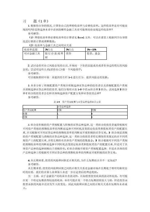
习题（1章）1.根据你自身的情况,计算你自己的理想收益率与必要收益率。

这些收益率是有可能实现的吗?你觉得选择本章中讲到的哪些金融工具有可能帮助你实现这些收益率?参考解答：（1）理想收益率和必要收益率的计算请见Excel文件，可以在课堂上根据同学自身情况进行模拟计算或调整数值。

2.试讨论你对自己风险态度的认识,并询问一下你的家庭成员或者你身边的朋友的风险态度。

尝试对这些人(包括你自己)做一个风险排序。

参考解答：可以根据教材中第一章提供的专栏1-1进行打分，提供风险态度依据。

3.本章分析了积极配置资产类别并积极选择证券品种的投资者以及消极配置资产类别并消极选择证券品种的投资者,他们分别对应表1-9中的A组合和D组合。

试问选择B组合和C组合的投资者会怎样具体地选择资产配置方案和证券投资品种?参考解答：表1-9 资产类别配置与证券品种选择组合示意A组合是积极的资产类别配置与积极的证券品种选择,这一类组合的投资者通常根据对不同资产类别的预期收益率的判断而选择不同时机改变固定收益类和股权类资产的配置比重,并且根据对不同证券品种的预期收益率的判断而开展积极的证券交易。

D组合则是消极的资产类别配置与消极的证券品种选择,这一类组合的投资者将长期坚持其既定的在不同类别资产上的配置比重,并将长期持有具体资产类别的指数基金。

B组合根据对不同资产类别的预期收益率的判断而选择不同时机改变固定收益类和股权类资产的配置比重,但是对于具体资产品种的选择则倾向于消极持有。

C组合消极开展资产类别配置选择，但是在具体的资产品种选择上将根据对不同证券品种的预期收益率的判断而开展积极的证券交易。

4.从长期来看,投资的风险和回报是正相关的,为什么短期而言并不一定如此?参考解答：从长期来看,投资的风险和回报之间的正相关关系是金融市场在长期处于相对均衡状态时的结果，我们将在第七章和第八章进一步讨论背后的理论机制。

另一方面，由于金融资产的收益具有波动性，比如股票投资收益的波动性较高，有可能在某一个特定短期获得较高的收益，也有可能在某一个特点短期招致较大亏损，但是投资该股票承担的风险并没有发生大的变化，因此风险和回报之间的正相关关系在短期内未必成立。

（完整版）投资学第10版习题答案05

（完整版）投资学第10版习题答案05CHAPTER 5: RISK, RETURN, AND THE HISTORICALRECORDPROBLEM SETS1. The Fisher equation predicts that the nominal rate will equal the equilibriumreal rate plus the expected inflation rate. Hence, if the inflation rate increasesfrom 3% to 5% while there is no change in the real rate, then the nominal ratewill increase by 2%. On the other hand, it is possible that an increase in theexpected inflation rate would be accompanied by a change in the real rate ofinterest. While it is conceivable that the nominal interest rate could remainconstant as the inflation rate increased, implying that the real rate decreasedas inflation increased, this is not a likely scenario.2. If we assume that the distribution of returns remains reasonably stable overthe entire history, then a longer sample period (i.e., a larger sample) increasesthe precision of the estimate of the expected rate of return; this is aconsequence of the fact that the standard error decreases as the sample sizeincreases. However, if we assume that the mean of the distribution of returnsis changing over time but we are not in a position to determine the nature ofthis change, then the expected return must be estimated from a more recentpart of the historical period. In this scenario, we must determine how far back,historically, to go in selecting the relevant sample. Here, it is likely to bedisadvantageous to use the entire data set back to 1880.3. The true statements are (c) and (e). The explanations follow.Statement (c): Let σ = the annual standard deviation of the risky investmentsand 1σ= the standard deviation of the first investment alternative over the two-year period. Then:σσ?=21Therefore, the annualized standard deviation for the first investment alternative is equal to:σσσ<=221Statement (e): The first investment alternative is more attractive to investors with lower degrees of risk aversion. The first alternative (entailing a sequence of two identically distributed and uncorrelated risky investments) is riskierthan the second alternative (the risky investment followed by a risk-freeinvestment). Therefore, the first alternative is more attractive to investors with lower degrees of risk aversion. Notice, however, that if you mistakenlybelieved that time diversification can reduce the total risk of a sequence ofrisky investments, you would have been tempted to conclude that the firstalternative is less risky and therefore more attractive to more risk-averseinvestors. This is clearly not the case; the two-year standard deviation of thefirst alternative is greater than the two-year standard deviation of the secondalternative.4. For the money market fund, your holding-period return for the next yeardepends on the level of 30-day interest rates each month when the fund rolls over maturing securities. The one-year savings deposit offers a 7.5% holding period return for the year. If you forecast that the rate on money marketinstruments will increase significantly above the current 6% yield, then themoney market fund might result in a higher HPR than the savings deposit.The 20-year Treasury bond offers a yield to maturity of 9% per year, which is 150 basis points higher than the rate on the one-year savings deposit; however, you could earn a one-year HPR much less than 7.5% on the bond if long-term interest rates increase during the year. If Treasury bond yields rise above 9%, then the price of the bond will fall, and the resulting capital loss will wipe out some or all of the 9% return you would have earned if bond yields hadremained unchanged over the course of the year.5. a. If businesses reduce their capital spending, then they are likely todecrease their demand for funds. This will shift the demand curve inFigure 5.1 to the left and reduce the equilibrium real rate of interest.b. Increased household saving will shift the supply of funds curve to theright and cause real interest rates to fall.c. Open market purchases of U.S. Treasury securities by the FederalReserve Board are equivalent to an increase in the supply of funds (ashift of the supply curve to the right). The FED buys treasuries withcash from its own account or it issues certificates which trade likecash. As a result, there is an increase in the money supply, and theequilibrium real rate of interest will fall.6. a. The “Inflation-Plus” CD is the safer investment because it guarantees thepurchasing power of the investment. Using the approximation that the realrate equals the nominal rate minus the inflation rate, the CD provides a realrate of 1.5% regardless of the inflation rate.b. The expected return depends on the expected rate of inflation over the nextyear. If the expected rate of inflation is less than 3.5% then the conventionalCD offers a higher real return than the inflation-plus CD; if the expected rateof inflation is greater than 3.5%, then the opposite is true.c. If you expect the rate of inflation to be 3% over the next year, then theconventional CD offers you an expected real rate of return of 2%, which is0.5% higher than the real rate on the inflation-protected CD. But unless youknow that inflation will be 3% with certainty, the conventional CD is alsoriskier. The question of which is the better investment then depends on yourattitude towards risk versus return. You might choose to diversify and investpart of your funds in each.d. No. We cannot assume that the entire difference between the risk-freenominal rate (on conventional CDs) of 5% and the real risk-free rate (oninflation-protected CDs) of 1.5% is the expected rate of inflation. Part of thedifference is probably a risk premium associated with the uncertaintysurrounding the real rate of return on the conventional CDs. This impliesthat the expected rate of inflation is less than 3.5% per year.7. E(r) = [0.35 × 44.5%] + [0.30 × 14.0%] + [0.35 × (–16.5%)] = 14%σ2 = [0.35 × (44.5 – 14)2] + [0.30 × (14 – 14)2] + [0.35 × (–16.5 – 14)2] = 651.175 σ = 25.52%The mean is unchanged, but the standard deviation has increased, as theprobabilities of the high and low returns have increased.8. Probability distribution of price and one-year holding period return for a 30-year U.S. Treasury bond (which will have 29 years to maturity at year-end):Economy Probability YTM Price CapitalGainCouponInterest HPRBoom 0.20 11.0% $ 74.05 -$25.95 $8.00 -17.95% Normal growth 0.50 8.0 100.00 0.00 8.00 8.00 Recession 0.30 7.0 112.28 12.28 8.00 20.289. E(q) = (0 × 0.25) + (1 × 0.25) + (2 × 0.50) = 1.25σq = [0.25 × (0 – 1.25)2 + 0.25 × (1 – 1.25)2 + 0.50 × (2 – 1.25)2]1/2 = 0.8292 10. (a) With probability 0.9544, the value of a normally distributedvariable will fall within 2 standard deviations of the mean; that is,between –40% and 80%. Simply add and subtract 2 standarddeviations to and from the mean.11. From Table 5.4, the average risk premium for the period 7/1926-9/2012 was:12.34% per year.Adding 12.34% to the 3% risk-free interest rate, the expected annual HPR for the Big/Value portfolio is: 3.00% + 12.34% = 15.34%.No. The distributions from (01/1928–06/1970) and (07/1970–12/2012) periods have distinct characteristics due to systematic shocks to the economy and subsequent government intervention. While the returns from the two periods do not differ greatly, their respective distributions tell a different story. The standard deviation for all six portfolios is larger in the first period. Skew is also positive, but negative in the second, showing a greater likelihood of higher-than-normal returns in the right tail.Kurtosis is also markedly larger in the first period.13. a%88.5,0588.070.170.080.01111or i i rn i rn rr =-=+-=-++=b. rr ≈ rn - i = 80% - 70% = 10%Clearly, the approximation gives a real HPR that is too high.14. From Table 5.2, the average real rate on T-bills has been 0.52%.a. T-bills: 0.52% real rate + 3% inflation = 3.52%b. Expected return on Big/Value:3.52% T-bill rate + 12.34% historical risk premium = 15.86%c. The risk premium on stocks remains unchanged. A premium, thedifference between two rates, is a real value, unaffected by inflation.15. Real interest rates are expected to rise. The investment activity will shiftthe demand for funds curve (in Figure 5.1) to the right. Therefore theequilibrium real interest rate will increase.16. a. Probability distribution of the HPR on the stock market and put:STOCK PUT State of theEconomyProbability Ending Price + Dividend HPR Ending Value HPR Excellent0.25 $ 131.00 31.00% $ 0.00 -100% Good0.45 114.00 14.00 $ 0.00 -100 Poor0.25 93.25 ?6.75 $ 20.25 68.75 Crash 0.05 48.00 -52.00 $ 64.00 433.33Remember that the cost of the index fund is $100 per share, and the costof the put option is $12.b. The cost of one share of the index fund plus a put option is $112. Theprobability distribution of the HPR on the portfolio is:State of the Economy Probability Ending Price + Put + DividendHPRExcellent 0.25 $ 131.00 17.0%= (131 - 112)/112 Good 0.45 114.00 1.8= (114 - 112)/112 Poor 0.25 113.50 1.3= (113.50 - 112)/112 Crash0.05 112.00 0.0 = (112 - 112)/112 c. Buying the put option guarantees the investor a minimum HPR of 0.0% regardless of what happens to the stock's price. Thus, it offers insuranceagainst a price decline.17. The probability distribution of the dollar return on CD plus call option is:State of theEconomy Probability Ending Valueof CDEnding Valueof CallCombinedValueExcellent 0.25 $ 114.00 $16.50 $130.50Good 0.45 114.00 0.00 114.00Poor 0.25 114.00 0.00 114.00Crash 0.05 114.00 0.00 114.0018.a.Total return of the bond is (100/84.49)-1 = 0.1836. With t = 10, the annualrate on the real bond is (1 + EAR) = = 1.69%.b.With a per quarter yield of 2%, the annual yield is = 1.0824, or8.24%. The equivalent continuously compounding (cc) rate is ln(1+.0824)= .0792, or 7.92%. The risk-free rate is 3.55% with a cc rate of ln(1+.0355)= .0349, or 3.49%. The cc risk premium will equal .0792 - .0349 = .0443, or4.433%.c.The appropriate formula is ,where . Using solver or goal seek, setting thetarget cell to the known effective cc rate by changing the unknown variance(cc) rate, the equivalent standard deviation (cc) is 18.03% (excel mayyield slightly different solutions).d.The expected value of the excess return will grow by 120 months (12months over a 10-year horizon). Therefore the excess return will be 120 ×4.433% = 531.9%. The expected SD grows by the square root of timeresulting in 18.03% × = 197.5%. The resulting Sharpe ratio is531.9/197.5 = 2.6929. Normsdist (-2.6929) = .0035, or a .35% probabilityof shortfall over a 10-year horizon.CFA PROBLEMS1. The expected dollar return on the investment in equities is $18,000 (0.6 × $50,000 + 0.4×?$30,000) compared to the $5,000 expected return for T-bills. Therefore, the expected risk premium is $13,000.2. E(r) = [0.2 × (?25%)] + [0.3 × 10%] + [0.5 × 24%] =10%3. E(r X) = [0.2 × (?20%)] + [0.5 × 18%] + [0.3 × 50%] =20%E(r Y) = [0.2 × (?15%)] + [0.5 × 20%] + [0.3 × 10%] =10%4. σX2 = [0.2 × (– 20 – 20)2] + [0.5 × (18 – 20)2] + [0.3 × (50 – 20)2] = 592σX = 24.33%σY2 = [0.2 × (– 15 – 10)2] + [0.5 × (20 – 10)2] + [0.3 × (10 – 10)2] = 175σY = 13.23%5. E(r) = (0.9 × 20%) + (0.1 × 10%) =19% $1,900 in returns6. The probability that the economy will be neutral is 0.50, or 50%. Given aneutral economy, the stock will experience poor performance 30% of thetime. The probability of both poor stock performance and a neutral economy is therefore: 0.30 × 0.50 = 0.15 = 15%7. E(r) = (0.1 × 15%) + (0.6 × 13%) + (0.3 × 7%) = 11.4%。

投资学习题三答案

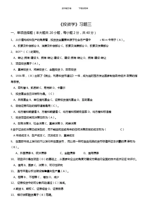
《投资学》习题三一、单项选择题（本大题共20小题，每小题2分，共40分）1、从价值构成和生产的角度看，投资资金重要来源于社会总产值中c和m中用于（A）。

A、积累及补偿部分B、消费及补偿部分C、积累及消费部分D、积累及发展部分2、BOT^（C）的简称。

A、转让-拥有-建设B、拥有-转让-建设C、建设-拥有-转让D、拥有-建设-转让3、项目投资属于（A）。

A、直接投资B、间接投资C、金融投资D、财政投资4、1936年，（B）出版了《就业、利息和货币通论》一书，成为当时西方发达国家制定政府经济政策的指导思想。

A、菲利普B、凯恩斯C、希克斯D、卡塞尔5、投资基金在日本被称为是。

（C）A、共同基金B、单位信托基金C、证券投资信托基金D、互助基金6、测定证券风险的指标通常是用（C）。

A、均方差和期望值B、方差和期望值C、均方差和预期收益率D、均方差和标准差7、投资项目的微观决策也称为（A）。

A、财务决策B、社会决策C、直接决策D、间接决策8由于过去的决策已经发生的，而不能由现在或将来的任何决策改变的成本称为（C）A 市场成本B、生产成本C、沉没成本D、直接成本9、在国际市场上发行的不以发行所在国货币，而以另一种可自由兑换的货币标值并还本伏羲的债券称为（B）。

A、外国债券B、欧洲债券C、金融债券D、信用债券10、项目评价是在项目（D）的基础上，从国家和企业的角度对建设方案进行全面的技术经济论证和评价。

A、信用B、国家C、决策D、可行性研究11、盈亏平衡分析法假设销售量和生产量（A）。

A、相等B 、不相等C 、增加D、减少12、证券投资中的可分散风险通过（C）消减。

A期货B、期权C、证券组合D、证券股息13、银行贷款融资属于（B）范畴。

A、直接融资B、间接融资C、股权融资D、信托融资14、按复利方式计算以后若干时期一定数量资金现在的价值称为（A）。

A、现值B、终值C、年金D、等值15、流动比率是流动资产与（A）的比率。

投资项目评估学东财附答案

一、单选题（共 15 道试题，共 60 分。

）1. （）是指在一定的规模下或一定的规模区间，企业生产最有效率A. 规模区间B. 规模经济C. 规模不经济D. 规模效率正确答案：B 满分：4 分得分：42.工厂化养猪不同于传统的养猪，由于实现了仔猪早期断奶，通过普遍使用早期断奶和人工授精技术，使得母猪年均产仔窝数达到了2.2～2.4窝，同时改变了过去季节产仔为常年产仔，既提高了猪崽产量，又使育肥猪全年均衡上市。

此项目属于（）A. 资金密集型B. 劳动密集型C. 技术密集型D. 知识密集型正确答案：C 满分：4 分得分：43. 生产能力是指企业在一定生产技术条件和一定时期内可能生产某种产品的（）A. 平均能力B. 最小能力C. 最大能力D. 抽样能力正确答案：C 满分：4 分得分：44. 不考虑资金来源的财务分析报表为()A. 财务现金流量表B. 资本金财务现金流量表C. 投资各方财务现金流量表D. 资金来源及运用表正确答案：A 满分：4 分得分：45. 以下属于项目财务现金流量表的项目有____A. 借款本金偿还B. 建设投资C. 所得税D. 股权投资正确答案：B 满分：4 分得分：46. （）分析是使用概率研究预测各种不确定因素和分险因素的发生对投资项目评价指标影响的一种定量分析方法A. 敏感性B. 概率C. 不确定性D. 盈亏平衡正确答案：B 满分：4 分得分：47. 原材料供应条件的评估必须对项目所需的全部原材料进行分析评价，以防“木桶效应”的出现A. 对B. 错正确答案：B 满分：4 分得分：48. 以下不能用损益和利润分配表计算的是____A. 投资利润率B. 投资利税率C. 内部收益率D. 资本金利润率正确答案：C 满分：4 分得分：49. 在无形资产的摊销中，对于法律和合同或者企业申请书分别规定有法定有效期和受益年限的，下面哪一个正确____A. 应以法律规定的法定有效期为准B. 应以合同或者企业申请书规定的受益年限为准C. 应以法定有效期与合同或者企业申请书规定的受益年限孰短的原则确定D. 没有规定期限的,应按不少于5年的期限分期摊销正确答案：C 满分：4 分得分：410. 总图的经济合理性是通过一系列的（）指标反映出来的A. 技术B. 技术经济C. 经济D. 考核正确答案：B 满分：4 分得分：411. 以下关于资本金现金流量表的说法正确的是____A. 所得税前资本金可能获得的收益水平B. 所得税后资本金可能获得的收益水平C. 所得税前可能获得的收益水平D. 所得税后可能获得的收益水平正确答案：B 满分：4 分得分：412. 对拟建项目的工艺技术方案分析评估，要求评估人员重复技术可行性研究，以确保技术切实可行A. 对B. 错正确答案：B 满分：4 分得分：413. 项目评估中确定拟建项目生产规模目的是使项目达到（）A. 规模不经济B. 规模经济正确答案：B 满分：4 分得分：414. （）阶段是市场分析能否充分发挥作用的关键一环A. 确定调查目标B. 制定调查计划C. 调查实施D. 调查结果处理正确答案：D 满分：4 分得分：415. 下列哪项不是决定投资的基本要素是（）A. 收益B. 成本C. 预期D. 政策正确答案：D 满分：4 分得分：4二、多选题（共 10 道试题，共 40 分。

投资学第10版课后习题答案

CHAPTER 7: OPTIMAL RISKY PORTFOLIOSPROBLEM SETS1. (a) and (e). Short-term rates and labor issues are factors thatare common to all firms and therefore must be considered as market risk factors. The remaining three factors are unique to this corporation and are not a part of market risk.2. (a) and (c). After real estate is added to the portfolio, there arefour asset classes in the portfolio: stocks, bonds, cash, and real estate. Portfolio variance now includes a variance term for real estate returns and a covariance term for real estate returns with returns for each of the other three asset classes. Therefore,portfolio risk is affected by the variance (or standard deviation) of real estate returns and the correlation between real estatereturns and returns for each of the other asset classes. (Note that the correlation between real estate returns and returns for cash is most likely zero.)3. (a) Answer (a) is valid because it provides the definition of theminimum variance portfolio.4. The parameters of the opportunity set are:E (r S ) = 20%, E (r B ) = 12%, σS = 30%, σB = 15%, ρ =From the standard deviations and the correlation coefficient we generate the covariance matrix [note that (,)S B S B Cov r r ρσσ=⨯⨯]: Bonds Stocks Bonds 225 45 Stocks 45 900The minimum-variance portfolio is computed as follows:w Min (S ) =1739.0)452(22590045225)(Cov 2)(Cov 222=⨯-+-=-+-B S B S B S B ,r r ,r r σσσ w Min (B ) = 1 =The minimum variance portfolio mean and standard deviation are:E (r Min ) = × .20) + × .12) = .1339 = %σMin = 2/12222)],(Cov 2[B S B S B B S Sr r w w w w ++σσ = [ 900) + 225) + (2 45)]1/2= %5.Proportion in Stock Fund Proportionin Bond Fund ExpectedReturnStandard Deviation% % % %minimumtangencyGraph shown below.0.005.0010.0015.0020.0025.000.00 5.00 10.00 15.00 20.00 25.00 30.00Tangency PortfolioMinimum Variance PortfolioEfficient frontier of risky assetsCMLINVESTMENT OPPORTUNITY SETr f = 8.006. The above graph indicates that the optimal portfolio is thetangency portfolio with expected return approximately % andstandard deviation approximately %.7. The proportion of the optimal risky portfolio invested in the stockfund is given by:222[()][()](,)[()][()][()()](,)S f B B f S B S S f B B f SS f B f S B E r r E r r Cov r r w E r r E r r E r r E r r Cov r r σσσ-⨯--⨯=-⨯+-⨯--+-⨯[(.20.08)225][(.12.08)45]0.4516[(.20.08)225][(.12.08)900][(.20.08.12.08)45]-⨯--⨯==-⨯+-⨯--+-⨯10.45160.5484B w =-=The mean and standard deviation of the optimal risky portfolio are:E (r P ) = × .20) + × .12) = .1561 = % σp = [ 900) +225) + (2× 45)]1/2= %8. The reward-to-volatility ratio of the optimal CAL is:().1561.080.4601.1654p fpE r r σ--==9. a. If you require that your portfolio yield an expected return of14%, then you can find the corresponding standard deviation from the optimal CAL. The equation for this CAL is:()().080.4601p fC f C C PE r r E r r σσσ-=+=+If E (r C ) is equal to 14%, then the standard deviation of the portfolio is %.b. To find the proportion invested in the T-bill fund, rememberthat the mean of the complete portfolio ., 14%) is an average of the T-bill rate and the optimal combination of stocks and bonds (P ). Let y be the proportion invested in the portfolio P . The mean of any portfolio along the optimal CAL is:()(1)()[()].08(.1561.08)C f P f P f E r y r y E r r y E r r y =-⨯+⨯=+⨯-=+⨯-Setting E (r C ) = 14% we find: y = and (1 − y ) = (the proportion invested in the T-bill fund).To find the proportions invested in each of the funds, multiply times the respective proportions of stocks and bonds in the optimal risky portfolio:Proportion of stocks in complete portfolio = =Proportion of bonds in complete portfolio = =10. Using only the stock and bond funds to achieve a portfolio expectedreturn of 14%, we must find the appropriate proportion in the stock fund (w S) and the appropriate proportion in the bond fund (w B = 1 −w S) as follows:= × w S + × (1 −w S) = + × w S w S =So the proportions are 25% invested in the stock fund and 75% inthe bond fund. The standard deviation of this portfolio will be:σP = [ 900) + 225) + (2 45)]1/2 = %This is considerably greater than the standard deviation of %achieved using T-bills and the optimal portfolio.11. a.Even though it seems that gold is dominated by stocks, gold mightstill be an attractive asset to hold as a part of a portfolio. Ifthe correlation between gold and stocks is sufficiently low, goldwill be held as a component in a portfolio, specifically, theoptimal tangency portfolio.b.If the correlation between gold and stocks equals +1, then no onewould hold gold. The optimal CAL would be composed of bills andstocks only. Since the set of risk/return combinations of stocksand gold would plot as a straight line with a negative slope (seethe following graph), these combinations would be dominated bythe stock portfolio. Of course, this situation could not persist.If no one desired gold, its price would fall and its expectedrate of return would increase until it became sufficientlyattractive to include in a portfolio.12. Since Stock A and Stock B are perfectly negatively correlated, arisk-free portfolio can be created and the rate of return for thisportfolio, in equilibrium, will be the risk-free rate. To find theproportions of this portfolio [with the proportion w A invested inStock A and w B = (1 –w A) invested in Stock B], set the standarddeviation equal to zero. With perfect negative correlation, theportfolio standard deviation is:σP = Absolute value [w AσA w BσB]0 = 5 × w A− [10 (1 –w A)] w A =The expected rate of return for this risk-free portfolio is:E(r) = × 10) + × 15) = %Therefore, the risk-free rate is: %13. False. If the borrowing and lending rates are not identical, then,depending on the tastes of the individuals (that is, the shape oftheir indifference curves), borrowers and lenders could havedifferent optimal risky portfolios.14. False. The portfolio standard deviation equals the weighted averageof the component-asset standard deviations only in the special case that all assets are perfectly positively correlated. Otherwise, as the formula for portfolio standard deviation shows, the portfoliostandard deviation is less than the weighted average of thecomponent-asset standard deviations. The portfolio variance is aweighted sum of the elements in the covariance matrix, with theproducts of the portfolio proportions as weights.15. The probability distribution is:Probability Rate ofReturn100%−50Mean = [ × 100%] + [ × (-50%)] = 55%Variance = [ × (100 − 55)2] + [ × (-50 − 55)2] = 4725Standard deviation = 47251/2 = %16. σP = 30 = y× σ = 40 × y y =E(r P) = 12 + (30 − 12) = %17. The correct choice is (c). Intuitively, we note that since allstocks have the same expected rate of return and standard deviation, we choose the stock that will result in lowest risk. This is thestock that has the lowest correlation with Stock A.More formally, we note that when all stocks have the same expected rate of return, the optimal portfolio for any risk-averse investor is the global minimum variance portfolio (G). When the portfolio is restricted to Stock A and one additional stock, the objective is to find G for any pair that includes Stock A, and then select thecombination with the lowest variance. With two stocks, I and J, theformula for the weights in G is:)(1)(),(Cov 2),(Cov )(222I w J w r r r r I w Min Min J I J I J I J Min -=-+-=σσσSince all standard deviations are equal to 20%:(,)400and ()()0.5I J I J Min Min Cov r r w I w J ρσσρ====This intuitive result is an implication of a property of any efficient frontier, namely, that the covariances of the global minimum variance portfolio with all other assets on the frontier are identical and equal to its own variance. (Otherwise, additional diversification would further reduce the variance.) In this case, the standard deviation of G(I, J) reduces to:1/2()[200(1)]Min IJ G σρ=⨯+This leads to the intuitive result that the desired addition would be the stock with the lowest correlation with Stock A, which is Stock D. The optimal portfolio is equally invested in Stock A and Stock D, and the standard deviation is %.18. No, the answer to Problem 17 would not change, at least as long asinvestors are not risk lovers. Risk neutral investors would not care which portfolio they held since all portfolios have an expected return of 8%.19. Yes, the answers to Problems 17 and 18 would change. The efficientfrontier of risky assets is horizontal at 8%, so the optimal CAL runs from the risk-free rate through G. This implies risk-averse investors will just hold Treasury bills.20. Rearrange the table (converting rows to columns) and compute serialcorrelation results in the following table:Nominal RatesFor example: to compute serial correlation in decade nominalreturns for large-company stocks, we set up the following twocolumns in an Excel spreadsheet. Then, use the Excel function“CORREL” to calculate the correlation for the data.Decade Previous1930s%%1940s%%1950s%%1960s%%1970s%%1980s%%1990s%%Note that each correlation is based on only seven observations, so we cannot arrive at any statistically significant conclusions.Looking at the results, however, it appears that, with theexception of large-company stocks, there is persistent serialcorrelation. (This conclusion changes when we turn to real rates in the next problem.)21. The table for real rates (using the approximation of subtracting adecade’s average inflation from the decade’s average nominalreturn) is:Real RatesSmall Company StocksLarge Company StocksLong-TermGovernmentBondsIntermed-TermGovernmentBondsTreasuryBills 1920s1930s1940s1950s1960s1970s1980s1990sSerialCorrelationWhile the serial correlation in decade nominal returns seems to be positive, it appears that real rates are serially uncorrelated. The decade time series (although again too short for any definitiveconclusions) suggest that real rates of return are independent from decade to decade.22. The 3-year risk premium for the S&P portfolio is, the 3-year risk premium for thehedge fund portfolio is S&P 3-year standard deviation is 0. The hedge fund 3-year standard deviation is 0. S&P Sharpe ratio is = , and the hedge fund Sharpe ratio is = .23. With a ρ = 0, the optimal asset allocation is,.With these weights,EThe resulting Sharpe ratio is = . Greta has a risk aversion of A=3, Therefore, she will investyof her wealth in this risky portfolio. The resulting investment composition will be S&P: = % and Hedge: = %. The remaining 26% will be invested in the risk-free asset.24. With ρ = , the annual covariance is .25. S&P 3-year standard deviation is . The hedge fund 3-year standard deviation is . Therefore, the 3-year covariance is 0.26. With a ρ=.3, the optimal asset allocation is, .With these weights,E. The resulting Sharpe ratio is = . Notice that the higher covariance results in a poorer Sharpe ratio.Greta will investyof her wealth in this risky portfolio. The resulting investment composition will be S&P: =% and hedge: = %. The remaining % will be invested in the risk-free asset.CFA PROBLEMS1. a. Restricting the portfolio to 20 stocks, rather than 40 to 50stocks, will increase the risk of the portfolio, but it ispossible that the increase in risk will be minimal. Suppose that, for instance, the 50 stocks in a universe have the same standard deviation () and the correlations between each pair areidentical, with correlation coefficient ρ. Then, the covariance between each pair of stocks would be ρσ2, and the variance of an equally weighted portfolio would be:222ρσ1σ1σnn n P -+=The effect of the reduction in n on the second term on theright-hand side would be relatively small (since 49/50 is close to 19/20 and ρσ2 is smaller than σ2), but thedenominator of the first term would be 20 instead of 50. For example, if σ = 45% and ρ = , then the standard deviation with 50 stocks would be %, and would rise to % when only 20 stocks are held. Such an increase might be acceptable if the expected return is increased sufficiently.b. Hennessy could contain the increase in risk by making sure thathe maintains reasonable diversification among the 20 stocks that remain in his portfolio. This entails maintaining a low correlation among the remaining stocks. For example, in part (a), with ρ = , the increase in portfolio risk was minimal. As a practical matter, this means that Hennessy would have to spread his portfolio among many industries; concentrating on just a few industries would result in higher correlations among the included stocks.2. Risk reduction benefits from diversification are not a linearfunction of the number of issues in the portfolio. Rather, the incremental benefits from additional diversification are mostimportant when you are least diversified. Restricting Hennessy to 10 instead of 20 issues would increase the risk of his portfolio by a greater amount than would a reduction in the size of theportfolio from 30 to 20 stocks. In our example, restricting the number of stocks to 10 will increase the standard deviation to %. The % increase in standard deviation resulting from giving up 10 of20 stocks is greater than the % increase that results from givingup 30 of 50 stocks.3. The point is well taken because the committee should be concernedwith the volatility of the entire portfolio. Since Hennessy’sportfolio is only one of six well-diversified portfolios and issmaller than the average, the concentration in fewer issues mighthave a minimal effect on the diversification of the total fund.Hence, unleashing Hennessy to do stock picking may be advantageous.4. d. Portfolio Y cannot be efficient because it is dominated byanother portfolio. For example, Portfolio X has both higherexpected return and lower standard deviation.5. c.6. d.7. b.8. a.9. c.10. Since we do not have any information about expected returns, wefocus exclusively on reducing variability. Stocks A and C have equal standard deviations, but the correlation of Stock B with Stock C is less than that of Stock A with Stock B . Therefore, a portfoliocomposed of Stocks B and C will have lower total risk than aportfolio composed of Stocks A and B.11. Fund D represents the single best addition to complementStephenson's current portfolio, given his selection criteria. Fund D’s expected return percent) has the potential to increase theportfolio’s return somewhat. Fund D’s relatively low correlation with his current portfolio (+ indicates that Fund D will providegreater diversification benefits than any of the other alternativesexcept Fund B. The result of adding Fund D should be a portfolio with approximately the same expected return and somewhat lower volatility compared to the original portfolio.The other three funds have shortcomings in terms of expected return enhancement or volatility reduction through diversification. Fund A offers the potential for increasing the portfolio’s return but is too highly correlated to provide substantial volatility reduction benefits through diversification. Fund B provides substantial volatility reduction through diversification benefits but is expected to generate a return well below the current portfolio’s return. Fund C has the greatest potential to increase the portfolio’s return but is too highly correlated with the current portfolio to provide substantial volatility reduction benefits through diversification.12. a. Subscript OP refers to the original portfolio, ABC to thenew stock, and NP to the new portfolio.i. E(r NP) = w OP E(r OP) + w ABC E(r ABC) = + = %ii. Cov = ρOP ABC = =iii. NP = [w OP2OP2 + w ABC2ABC2 + 2 w OP w ABC(Cov OP , ABC)]1/2= [ 2 + + (2 ]1/2= % %b. Subscript OP refers to the original portfolio, GS to governmentsecurities, and NP to the new portfolio.i. E(r NP) = w OP E(r OP) + w GS E(r GS) = + = %ii. Cov = ρOP GS = 0 0 = 0iii. NP = [w OP2OP2 + w GS2GS2 + 2 w OP w GS (Cov OP , GS)]1/2= [ + 0) + (2 0)]1/2= % %c. Adding the risk-free government securities would result in alower beta for the new portfolio. The new portfolio beta will bea weighted average of the individual security betas in theportfolio; the presence of the risk-free securities would lowerthat weighted average.d. The comment is not correct. Although the respective standarddeviations and expected returns for the two securities underconsideration are equal, the covariances between each security andthe original portfolio are unknown, making it impossible to drawthe conclusion stated. For instance, if the covariances aredifferent, selecting one security over the other may result in alower standard deviation for the portfolio as a whole. In such acase, that security would be the preferred investment, assumingall other factors are equal.e. i. Grace clearly expressed the sentiment that the risk of losswas more important to her than the opportunity for return. Usingvariance (or standard deviation) as a measure of risk in her casehas a serious limitation because standard deviation does notdistinguish between positive and negative price movements.ii. Two alternative risk measures that could be used instead ofvariance are:Range of returns, which considers the highest and lowestexpected returns in the future period, with a larger rangebeing a sign of greater variability and therefore of greaterrisk.Semivariance can be used to measure expected deviations ofreturns below the mean, or some other benchmark, such as zero.Either of these measures would potentially be superior tovariance for Grace. Range of returns would help to highlightthe full spectrum of risk she is assuming, especially thedownside portion of the range about which she is so concerned.Semivariance would also be effective, because it implicitlyassumes that the investor wants to minimize the likelihood ofreturns falling below some target rate; in Grace’s case, thetarget rate would be set at zero (to protect against negativereturns).13. a. Systematic risk refers to fluctuations in asset prices causedby macroeconomic factors that are common to all risky assets;hence systematic risk is often referred to as market risk.Examples of systematic risk factors include the business cycle,inflation, monetary policy, fiscal policy, and technologicalchanges.Firm-specific risk refers to fluctuations in asset pricescaused by factors that are independent of the market, such asindustry characteristics or firm characteristics. Examples offirm-specific risk factors include litigation, patents,management, operating cash flow changes, and financial leverage.b. Trudy should explain to the client that picking only the topfive best ideas would most likely result in the client holdinga much more risky portfolio. The total risk of a portfolio, orportfolio variance, is the combination of systematic risk andfirm-specific risk.The systematic component depends on the sensitivity of theindividual assets to market movements as measured by beta.Assuming the portfolio is well diversified, the number ofassets will not affect the systematic risk component ofportfolio variance. The portfolio beta depends on theindividual security betas and the portfolio weights of those securities.On the other hand, the components of firm-specific risk (sometimes called nonsystematic risk) are not perfectly positively correlated with each other and, as more assets are added to the portfolio, those additional assets tend to reduce portfolio risk. Hence, increasing the number of securities in a portfolio reduces firm-specific risk. For example, a patent expiration for one company would not affect the othersecurities in the portfolio. An increase in oil prices islikely to cause a drop in the price of an airline stock butwill likely result in an increase in the price of an energy stock. As the number of randomly selected securities increases, the total risk (variance) of the portfolio approaches its systematic variance.。

投资学第10版课后习题答案.docx

CHAPTER 4: MUTUAL FUNDS AND OTHER INVESTMENTCOMPANIESPROBLEM SETS1.The unit investment trust should have lower operating expenses.Because the investment trust portfolio is fixed once the trust isestablished, it does not have to pay portfolio managers toconstantly monitor and rebalance the portfolio as perceivedneeds or opportunities change. Because the portfolio is fixed, theunit investment trust also incurs virtually no trading costs.2. a. Unit investment trusts : Diversification from large-scale investing,lower transaction costs associated with large-scale trading, lowmanagement fees, predictable portfolio composition, guaranteed lowportfolio turnover rate.b.Open-end mutual funds : Diversification from large-scaleinvesting, lower transaction costs associated with large-scale trading, professional management that may be able totake advantage of buy or sell opportunities as they arise,record keeping.c.Individual stocks and bonds: No management fee; ability tocoordinate realization of capital gains or losses withinvestors ’ personal tax situation s; capability of designingportfolio to investor’s specific risk and return profile.3.Open-end funds are obligated to redeem investor's shares at netasset value and thus must keep cash or cash-equivalent securitieson hand in order to meet potential redemptions. Closed-end fundsdo not need the cash reserves because there are no redemptions forclosed-end funds. Investors in closed-end funds sell their shareswhen they wish to cash out.4.Balanced funds keep relatively stable proportions of funds investedin each asset class. They are meant as convenient instruments toprovide participation in a range of asset classes. Life-cycle fundsare balanced funds whose asset mix generally depends on the age of the investor. Aggressive life-cycle funds, with larger investments in equities, are marketed to younger investors, while conservative life-cycle funds, with larger investments in fixed-income securities, are designed for older investors. Asset allocation funds, in contrast, may vary the proportions invested in each asset class by large amounts as predictions of relative performance across classes vary. Asset allocation funds therefore engage in more aggressive market timing.5.Unlike an open-end fund, in which underlying shares are redeemedwhen the fund is redeemed, a closed-end fund trades as a security in the market. Thus, their prices may differ from the NAV.6.Advantages of an ETF over a mutual fund:ETFs are continuously traded and can be sold or purchasedon margin.There are no capital gains tax triggers when an ETF issold (shares are just sold from one investor to another).Investors buy from brokers, thus eliminating the cost ofdirect marketing to individual small investors. Thisimplies lower management fees.Disadvantages of an ETF over a mutual fund:Prices can depart from NAV (unlike an open-end fund).There is a broker fee when buying and selling (unlike ano-load fund).7.The offering price includes a 6% front-end load, or salescommission, meaning that every dollar paid results in only$ going toward purchase of shares. Therefore:Offering price =NAV$10.70 = $1Load 1 0.068.NAV = Offering price(1–Load) = $.95 = $9.Stock Value Held by FundA$ 7,000,000B12,000,000C8,000,000D15,000,000Total $42,000,000Net asset value =$42,000,000$30,000 = $4,000,00010.Value of stocks sold and replaced = $15,000,000Turnover rate =$15,000,000= , or % $42,000,00011. a.$200,000,000$3,000,000NAV$39.405,000,000b.Premium (or discount) =Pr ice NAV =$36$39.40 =–, or %NAV$39.40 The fund sells at an % discount from NAV.NAV 1 NAV 0 Distributions$12.10$12.50$1.50 12.$12.500.088, or 8.8%NAV 013. a. Start-of-year price:P0 = $×= $End-of-year price:P = $ × = $1Although NAV increased by $, the price of the fund decreased by$.Rate of return =P P Distributions$11.25$12.24$1.50100.042, or 4.2%P0$12.24b.An investor holding the same securities as the fund managerwould have earned a rate of return based on the increase inthe NAV of the portfolio:NAV 1 NAV 0 Distributions$12.10$12.00$1.50NAV 0$12.000.133, or 13.3%14. a. Empirical research indicates that past performance of mutualfunds is not highly predictive of future performance,especially for better-performing funds. While there maybe some tendency for the fund to be an above average performer nextyear, it is unlikely to once again be a top 10% performer.b.On the other hand, the evidence is more suggestive of atendency for poor performance to persist. This tendency isprobably related to fund costs and turnover rates. Thus ifthe fund is among the poorest performers, investors shouldbe concerned that the poor performance will persist.15.NAV0 = $200,000,000/10,000,000 = $20Dividends per share = $2,000,000/10,000,000 = $NAV is based on the 8% price gain, less the 1% 12b-1 fee: 1NAV1 = $20(1 – = $Rate of return =$21.384 $20$0.20 = , or %$2016.The excess of purchases over sales must be due to new inflowsinto the fund. Therefore, $400 million of stock previously held by thefund was replaced by new holdings. So turnover is: $400/$2,200 = ,or %.17. Fees paid to investment managers were: $ billion = $ million Since thetotal expense ratio was % and the management fee was %, weconclude that % must be for other expenses. Therefore, otheradministrative expenses were:$ billion = $ million.18.As an initial approximation, your return equals the return on the sharesminus the total of the expense ratio and purchase costs: 12%%4% = %.But the precise return is less than this because the 4% loadis paid up front, not at the end of the year.To purchase the shares, you would have had to invest:$20,000/(1 = $20,833.The shares increase in value from $20,000 to:= $20,000 $22,160.The rate of return is: ($22,160$20,833)/$20,833 = %.19.Assume $1,000 investment Loaded-Up Fund Economy Fund Yearly growth ( r is 6%)(1 r .01 .0075)(.98) (1 r .0025) t= 1 year$1,$1,t= 3 years$1,$1,t= 10 years$1,$1,20.a. $450,000,000 $10,000000 $1044,000,000b. The redemption of 1 million shares will most likely trigger capitalgains taxes which will lower the remaining portfolio by an amountgreater than $10,000,000 (implying a remaining total value lessthan $440,000,000). The outstanding shares fall to 43 million andthe NAV drops to below $10.21.Suppose you have $1,000 to invest. The initial investment inClass A shares is $940 net of the front-end load. After four years,your portfolio will be worth:$940 4 = $1,Class B shares allow you to invest the full $1,000, but yourinvestment performance net of 12b-1 fees will be only %, andyou will pay a 1% back-end load fee if you sell after four years.Your portfolio value after four years will be:$1,000 4 = $1,After paying the back-end load fee, your portfolio value will be:$1,.99 = $1,Class B shares are the better choice if your horizon is four years.With a 15-year horizon, the Class A shares will be worth:$94015 = $3,For the Class B shares, there is no back-end load in this casesince the horizon is greater than five years. Therefore, thevalue of the Class B shares will be:$1,00015 = $3,At this longer horizon, Class B shares are no longer the betterchoice. The effect of Class B's % 12b-1 fees accumulates over timeand finally overwhelms the 6% load charged to Class A investors.22. a.After two years, each dollar invested in a fund with a 4%load and a portfolio return equal to r will grow to: $ 2.(1 +r–Each dollar invested in the bank CD will grow to: $1.If the mutual fund is to be the better investment, thenthe portfolio return ( r ) must satisfy:(1 +r –2>(1 +r – 2 >(1 + r–2>1 + r – >1 + r >Therefore: r > = %b.If you invest for six years, then the portfolio returnmust satisfy:(1 + r –6 > =(1 +r–6>1 +r–>r > %The cutoff rate of return is lower for the six-year investment because the “fixed cost ” (the one -time front-end load) is spread over a greater number of years.c. With a 12b-1 fee instead of a front-end load, the portfoliomust earn a rate of return ( r ) that satisfies:1 + r – – >In this case, r must exceed % regardless of the investmenthorizon.23. The turnover rate is 50%. This means that, on average, 50% of theportfolio is sold and replaced with other securities each year.Trading costs on the sell orders are % and the buy orders toreplace those securities entail another % in trading costs. Totaltrading costs will reduce portfolio returns by: 2 % = %24. For the bond fund, the fraction of portfolio income given upto fees is:0.6% 4.0%= , or %For the equity fund, the fraction of investment earnings givenup to fees is:0. 6% = , or %12.0%Fees are a much higher fraction of expected earnings for thebond fund and therefore may be a more important factor inselecting the bond fund.This may help to explain why unmanaged unit investment trusts are concentrated in the fixed income market. The advantages of unitinvestment trusts are low turnover, low trading costs, and lowmanagement fees. This is a more important concern to bond-market investors.25. Suppose that finishing in the top half of all portfolio managersis purely luck, and that the probability of doing so in any year isexactly ? . Then the probability that any particular manager would5 = finish in the top half of the sample five years in a row is (?)1/32. We would then expect to find that [350 (1/32)] = 11managers finish in the top half for each of the five consecutiveyears. This is precisely what we found. Thus, we should not conclude that the consistent performance after five years is proof of skill. We would expect to find 11 managers exhibiting precisely this level of "consistency" even if performance is due solely to luck.。

投资学第10版课后习题答案

投资学第10版课后习题答案CHAPTER 7: OPTIMAL RISKY PORTFOLIOSPROBLEM SETS1. (a) and (e). Short-term rates and labor issues are factors thatare common to all firms and therefore must be considered as market risk factors. The remaining three factors are unique to this corporation and are not a part of market risk.2. (a) and (c). After real estate is added to the portfolio, there arefour asset classes in the portfolio: stocks, bonds, cash, and real estate. Portfolio variance now includes a variance term for real estate returns and a covariance term for real estate returns with returns for each of the other three asset classes. Therefore, portfolio risk is affected by the variance (or standard deviation) of real estate returns and the correlation between real estatereturns and returns for each of the other asset classes. (Note that the correlation between real estate returns and returns for cash is most likely zero.)3. (a) Answer (a) is valid because it provides the definition of theminimum variance portfolio.4. The parameters of the opportunity set are:E (r S ) = 20%, E (r B ) = 12%, σS = 30%, σB = 15%, ρ =From the standard deviations and the correlation coefficient we generate the covariance matrix [note that (,)S B S B Cov r r ρσσ=??]: Bonds Stocks Bonds 225 45 Stocks 45 900The minimum-variance portfolio is computed as follows:w Min (S ) =1739.0)452(22590045225)(Cov 2)(Cov 222=?-+-=-+-B S B S B S B ,r r ,r r σσσ w Min (B ) = 1 =The minimum variance portfolio mean and standard deviation are:E (r Min ) = × .20) + × .12) = .1339 = %σMin = 2/12222)],(Cov 2[B S B S B B S Sr r w w w w ++σσ = [ 900) + 225) + (2 45)]1/2= %5.Proportion in Stock Fund Proportionin Bond Fund ExpectedReturnStandard Deviation% % % %minimumtangencyGraph shown below.0.005.0010.0015.0020.0025.000.00 5.00 10.00 15.00 20.00 25.00 30.00Tangency PortfolioMinimum Variance PortfolioEfficient frontier of risky assetsCMLINVESTMENT OPPORTUNITY SETr f = 8.006. The above graph indicates that the optimal portfolio is thetangency portfolio with expected return approximately % andstandard deviation approximately %.7. The proportion of the optimal risky portfolio invested in the stockfund is given by:222[()][()](,)[()][()][()()](,)S f B B f S B S S f B B f SS f B f S B E r r E r r Cov r r w E r r E r r E r r E r r Cov r r σσσ-?--?=-?+-?--+-?[(.20.08)225][(.12.08)45]0.4516[(.20.08)225][(.12.08)900][(.20.08.12.08)45]-?--?==-?+-?--+-?10.45160.5484B w =-=The mean and standard deviation of the optimal risky portfolio are:E (r P ) = × .20) + × .12) = .1561 = % σp = [ 900) +225) + (2× 45)]1/2= %8. The reward-to-volatility ratio of the optimal CAL is:().1561.080.4601.1654p fpE r r σ--==9. a. If you require that your portfolio yield an expected return of14%, then you can find the corresponding standard deviation from the optimal CAL. The equation for this CAL is:()().080.4601p fC f C C PE r r E r r σσσ-=+=+If E (r C ) is equal to 14%, then the standard deviation of the portfolio is %.b. To find the proportion invested in the T-bill fund, rememberthat the mean of the complete portfolio ., 14%) is an average of the T-bill rate and the optimal combination of stocks and bonds (P ). Let y be the proportion invested in the portfolio P . The mean of any portfolio along the optimal CAL is:()(1)()[()].08(.1561.08)C f P f P f E r y r y E r r y E r r y =-?+?=+?-=+?-Setting E (r C ) = 14% we find: y = and (1 ? y ) = (the proportion invested in the T-bill fund).To find the proportions invested in each of the funds, multiply times the respective proportions of stocks and bonds in the optimal risky portfolio:Proportion of stocks in complete portfolio = =Proportion of bonds in complete portfolio = =10. Using only the stock and bond funds to achieve a portfolio expectedreturn of 14%, we must find the appropriate proportion in the stock fund (w S) and the appropriate proportion in the bond fund (w B = 1 ?w S) as follows:= × w S + × (1 ?w S) = + × w S w S =So the proportions are 25% invested in the stock fund and 75% inthe bond fund. The standard deviation of this portfolio will be:σP = [ 900) + 225) + (2 45)]1/2 = %This is considerably greater than the standard deviation of % achieved using T-bills and the optimal portfolio.11. a.Even though it seems that gold is dominated by stocks, gold mightstill be an attractive asset to hold as a part of a portfolio. If the correlation between gold and stocks is sufficiently low, goldwill be held as a component in a portfolio, specifically, the optimal tangency portfolio.b.If the correlation between gold and stocks equals +1, then no onewould hold gold. The optimal CAL would be composed of bills andstocks only. Since the set of risk/return combinations of stocksand gold would plot as a straight line with a negative slope (seethe following graph), these combinations would be dominated bythe stock portfolio. Of course, this situation could not persist.If no one desired gold, its price would fall and its expected rate of return would increase until it became sufficientlyattractive to include in a portfolio.12. Since Stock A and Stock B are perfectly negatively correlated, arisk-free portfolio can be created and the rate of return for thisportfolio, in equilibrium, will be the risk-free rate. To find the proportions of this portfolio [with the proportion w A invested inStock A and w B = (1 –w A) invested in Stock B], set the standarddeviation equal to zero. With perfect negative correlation, theportfolio standard deviation is:σP = Absolute value [w AσA w BσB]0 = 5 × w A? [10 (1 –w A)] w A =The expected rate of return for this risk-free portfolio is:E(r) = × 10) + × 15) = %Therefore, the risk-free rate is: %13. False. If the borrowing and lending rates are not identical, then,depending on the tastes of the individuals (that is, the shape oftheir indifference curves), borrowers and lenders could have different optimal risky portfolios.14. False. The portfolio standard deviation equals the weighted averageof the component-asset standard deviations only in the special case that all assets are perfectly positively correlated. Otherwise, as the formula for portfolio standard deviation shows, the portfoliostandard deviation is less than the weighted average of the component-asset standard deviations. The portfolio variance is aweighted sum of the elements in the covariance matrix, with theproducts of the portfolio proportions as weights.15. The probability distribution is:Probability Rate ofReturn100%50Mean = [ × 100%] + [ × (-50%)] = 55%Variance = [ × (100 ? 55)2] + [ × (-50 ? 55)2] = 4725Standard deviation = 47251/2 = %16. σP = 30 = y× σ = 40 × y y =E(r P) = 12 + (30 ? 12) = %17. The correct choice is (c). Intuitively, we note that since allstocks have the same expected rate of return and standard deviation, we choose the stock that will result in lowest risk. This is thestock that has the lowest correlation with Stock A.More formally, we note that when all stocks have the same expected rate of return, the optimal portfolio for any risk-averse investor is the global minimum variance portfolio (G). When the portfolio is restricted to Stock A and one additional stock, the objective is to find G for any pair that includes Stock A, and then select thecombination with the lowest variance. With two stocks, I and J, theformula for the weights in G is:)(1)(),(Cov 2),(Cov )(222I w J w r r r r I w Min Min J I J I J I J Min -=-+-=σσσSince all standard deviations are equal to 20%:(,)400and ()()0.5I J I J Min Min Cov r r w I w J ρσσρ====This intuitive result is an implication of a property of any efficient frontier, namely, that the covariances of the global minimum variance portfolio with all other assets on the frontier are identical and equal to its own variance. (Otherwise, additional diversification would further reduce the variance.) In this case, the standard deviation of G(I, J) reduces to:1/2()[200(1)]Min IJ G σρ=?+This leads to the intuitive result that the desired addition would be the stock with the lowest correlation with Stock A, which is Stock D. The optimal portfolio is equally invested in StockA and Stock D, and the standard deviation is %.18. No, the answer to Problem 17 would not change, at least as long asinvestors are not risk lovers. Risk neutral investors would not care which portfolio they held since all portfolios have an expected return of 8%.19. Yes, the answers to Problems 17 and 18 would change. The efficientfrontier of risky assets is horizontal at 8%, so the optimal CAL runs from the risk-free rate through G. This implies risk-averse investors will just hold Treasury bills.20. Rearrange the table (converting rows to columns) and compute serialcorrelation results in the following table:Nominal RatesFor example: to compute serial correlation in decade nominalreturns for large-company stocks, we set up the following twocolumns in an Excel spreadsheet. Then, use the Excel function“CORREL” to calculate the correlation for the data.Decade Previous1930s%%1940s%%1950s%%1960s%%1970s%%1980s%%1990s%%Note that each correlation is based on only seven observations, so we cannot arrive at any statistically significant conclusions.Looking at the results, however, it appears that, with theexception of large-company stocks, there is persistent serial correlation. (This conclusion changes when we turn to real rates in the next problem.)21. The table for real rates (using the approximation of subtracting adecade’s average inflation from the decade’s average nominalreturn) is:Real RatesSmall Company StocksLarge Company StocksLong-TermGovernmentBondsIntermed-TermGovernmentBondsTreasuryBills 1920s1930s1940s1950s1960s1970s1980s1990sSerialCorrelationWhile the serial correlation in decade nominal returns seems to be positive, it appears that real rates are serially uncorrelated. The decade time series (although again too short for any definitiveconclusions) suggest that real rates of return are independent from decade to decade.22. The 3-year risk premium for the S&P portfolio is, the 3-year risk premium for thehedge fund portfolio is S&P 3-year standard deviation is 0. The hedge fund 3-year standard deviation is 0. S&P Sharpe ratio is = , and the hedge fund Sharpe ratio is = .23. With a ρ = 0, the optimal asset allocation is,.With these weights,EThe resulting Sharpe ratio is = . Greta has a risk aversion of A=3, Therefore, she will investyof her wealth in this risky portfolio. The resulting investment composition will be S&P: = % and Hedge: = %. The remaining 26% will be invested in the risk-free asset.24. With ρ = , the annual covariance is .25. S&P 3-year standard deviation is . The hedge fund 3-year standard deviation is . Therefore, the 3-year covariance is 0.26. With a ρ=.3, the optimal asset allocation is, .With these weights,E. The resulting Sharpe ratio is = . Notice that the higher covariance results in a poorer Sharpe ratio.Greta will investyof her wealth in this risky portfolio. The resulting investment composition will be S&P: =% and hedge: = %. The remaining % will be invested in the risk-free asset.CFA PROBLEMS1. a. Restricting the portfolio to 20 stocks, rather than 40 to 50stocks, will increase the risk of the portfolio, but it ispossible that the increase in risk will be minimal. Suppose that, for instance, the 50 stocks in a universe have the samestandard deviation () and the correlations between each pair are identical, with correlation coefficient ρ. Then, the covariance between each pair of stocks would be ρσ2, and the variance of an equally weighted portfolio would be:222ρσ1σ1σnn n P -+=The effect of the reduction in n on the second term on the right-hand side would be relatively small (since 49/50 is close to 19/20 and ρσ2 is smaller than σ2), but thedenominator of the first term would be 20 instead of 50. For example, if σ = 45% and ρ = , then the standard deviation with 50 stocks would be %, and would rise to % when only 20 stocks are held. Such an increase might be acceptable if the expected return is increased sufficiently.b. Hennessy could contain the increase in risk by making sure thathe maintains reasonable diversification among the 20 stocks that remain in his portfolio. This entails maintaining a low correlation among the remaining stocks. For example, in part (a), with ρ = , the increase in portfolio risk was minimal. As a practical matter, this means that Hennessy would have to spread his portfolio among many industries; concentrating on just a few industries would result in higher correlations among the included stocks.2. Risk reduction benefits from diversification are not a linearfunction of the number of issues in the portfolio. Rather, the incremental benefits from additional diversification are most important when you are least diversified. Restricting Hennessy to 10 instead of 20 issues would increase the risk of hisportfolio by a greater amount than would a reduction in the size of theportfolio from 30 to 20 stocks. In our example, restricting the number of stocks to 10 will increase the standard deviation to %. The % increase in standard deviation resulting from giving up 10 of20 stocks is greater than the % increase that results from givingup 30 of 50 stocks.3. The point is well taken because the committee should be concernedwith the volatility of the entire portfolio. Since Hennessy’s portfolio is only one of six well-diversified portfolios and is smaller than the average, the concentration in fewer issues mighthave a minimal effect on the diversification of the total fund.Hence, unleashing Hennessy to do stock picking may be advantageous.4. d. Portfolio Y cannot be efficient because it is dominated byanother portfolio. For example, Portfolio X has both higher expected return and lower standard deviation.5. c.6. d.7. b.8. a.9. c.10. Since we do not have any information about expected returns, wefocus exclusively on reducing variability. Stocks A and C haveequal standard deviations, but the correlation of Stock B with Stock C is less than that of Stock A with Stock B . Therefore, a portfoliocomposed of Stocks B and C will have lower total risk than a portfolio composed of Stocks A and B.11. Fund D represents the single best addition to complementStephenson's current portfolio, given his selection criteria. Fund D’s expected return percent) has the potential to increase theportfolio’s return somewhat. Fund D’s relatively low correlation with his current portfolio (+ indicates that Fund D will providegreater diversification benefits than any of the other alternativesexcept Fund B. The result of adding Fund D should be a portfolio with approximately the same expected return and somewhat lower volatility compared to the original portfolio.The other three funds have shortcomings in terms of expected return enhancement or volatility reduction through diversification. Fund A offers the potential for increasing the portfolio’s return but is too highly correlated to provide substantial volatility reduction benefits through diversification. Fund B provides substantial volatility reduction through diversification benefits but is expected to generate a return well below the current portfolio’s return. Fund C has the greatest potential to increase th e portfolio’s return but is too highly correlated with the current portfolio to provide substantial volatility reduction benefits through diversification.12. a. Subscript OP refers to the original portfolio, ABC to thenew stock, and NP to the new portfolio.i. E(r NP) = w OP E(r OP) + w ABC E(r ABC) = + = %ii. Cov = ρOP ABC = =iii. NP = [w OP2OP2 + w ABC2ABC2 + 2 w OP w ABC(Cov OP , ABC)]1/2= [ 2 + + (2 ]1/2= % %b. Subscript OP refers to the original portfolio, GS to governmentsecurities, and NP to the new portfolio.i. E(r NP) = w OP E(r OP) + w GS E(r GS) = + = %ii. Cov = ρOP GS = 0 0 = 0iii. NP = [w OP2OP2 + w GS2GS2 + 2 w OP w GS (Cov OP , GS)]1/2= [ + 0) + (2 0)]1/2= % %c. Adding the risk-free government securities would result in alower beta for the new portfolio. The new portfolio beta will bea weighted average of the individual security betas in theportfolio; the presence of the risk-free securities would lower that weighted average.d. The comment is not correct. Although the respective standarddeviations and expected returns for the two securities under consideration are equal, the covariances between each security andthe original portfolio are unknown, making it impossible to drawthe conclusion stated. For instance, if the covariances aredifferent, selecting one security over the other may result in alower standard deviation for the portfolio as a whole. In such acase, that security would be the preferred investment, assumingall other factors are equal.e. i. Grace clearly expressed the sentiment that the risk of losswas more important to her than the opportunity for return. Usingvariance (or standard deviation) as a measure of risk in her casehas a serious limitation because standard deviation does not distinguish between positive and negative price movements.ii. Two alternative risk measures that could be used instead ofvariance are:Range of returns, which considers the highest and lowestexpected returns in the future period, with a larger rangebeing a sign of greater variability and therefore of greaterrisk.Semivariance can be used to measure expected deviations of returns below the mean, or some other benchmark, such as zero.Either of these measures would potentially be superior tovariance for Grace. Range of returns would help to highlight the full spectrum of risk she is assuming, especially thedownside portion of the range about which she is so concerned.Semivariance would also be effective, because it implicitlyassumes that the investor wants to minimize the likelihood ofreturns falling below some target rate; in Grace’s case, the target rate would be set at zero (to protect against negative returns).13. a. Systematic risk refers to fluctuations in asset prices causedby macroeconomic factors that are common to all risky assets;hence systematic risk is often referred to as market risk.Examples of systematic risk factors include the business cycle, inflation, monetary policy, fiscal policy, and technologicalchanges.Firm-specific risk refers to fluctuations in asset pricescaused by factors that are independent of the market, such asindustry characteristics or firm characteristics. Examples offirm-specific risk factors include litigation, patents,management, operating cash flow changes, and financial leverage.b. Trudy should explain to the client that picking only the topfive best ideas would most likely result in the client holdinga much more risky portfolio. The total risk of a portfolio, orportfolio variance, is the combination of systematic risk and firm-specific risk.The systematic component depends on the sensitivity of the individual assets to market movements as measured by beta.Assuming the portfolio is well diversified, the number ofassets will not affect the systematic risk component ofportfolio variance. The portfolio beta depends on theindividual security betas and the portfolio weights of those securities.On the other hand, the components of firm-specific risk (sometimes called nonsystematic risk) are not perfectly positively correlated with each other and, as more assets are added to the portfolio, those additional assets tend to reduce portfolio risk. Hence, increasing the number of securities in a portfolio reduces firm-specific risk. For example, a patent expiration for one company would not affect the othersecurities in the portfolio. An increase in oil prices islikely to cause a drop in the price of an airline stock butwill likely result in an increase in the price of an energy stock. As the number of randomly selected securities increases, the total risk (variance) of the portfolio approaches its systematic variance.。

投资学10版习题答案

CHAPTER 14: BOND PRICES AND YIELDSPROBLEM SETS1. a. Catastrophe bond—A bond that allows the issuer to transfer“catastrophe risk” from the firm to the capital markets. Investors inthese bonds receive a compensation for taking on the risk in the form ofhigher coupon rates. In the event of a catastrophe, the bondholders willreceive only part or perhaps none of the principal payment due to themat maturity. Disaster can be defined by total insured losses or by criteriasuch as wind speed in a hurricane or Richter level in an earthquake.b. Eurobond—A bond that is denominated in one currency, usually thatof the issuer, but sold in other national markets.c. Zero-coupon bond—A bond that makes no coupon payments. Investorsreceive par value at the maturity date but receive no interest paymentsuntil then. These bonds are issued at prices below par value, and theinvestor’s return comes from the difference between issue price and thepayment of par value at maturity (capital gain).d. Samurai bond—Yen-dominated bonds sold in Japan by non-Japaneseissuers.e. Junk bond—A bond with a low credit rating due to its high default risk;also known as high-yield bonds.f. Convertible bond—A bond that gives the bondholders an option toexchange the bond for a specified number of shares of common stock ofthe firm.g. Serial bonds—Bonds issued with staggered maturity dates. As bondsmature sequentially, the principal repayment burden for the firm isspread over time.h. Equipment obligation bond—A collateralized bond for which thecollateral is equipment owned by the firm. If the firm defaults on thebond, the bondholders would receive the equipment.i. Original issue discount bond—A bond issued at a discount to the facevalue.j. Indexed bond— A bond that makes payments that are tied to ageneral price index or the price of a particular commodity.k. Callable bond—A bond that gives the issuer the option to repurchase the bond at a specified call price before the maturity date.l. Puttable bond —A bond that gives the bondholder the option to sell back the bond at a specified put price before the maturity date.2. The bond callable at 105 should sell at a lower price because the call provision is more valuable to the firm. Therefore, its yield to maturity should be higher.3.Zero coupon bonds provide no coupons to be reinvested. Therefore, the investor's proceeds from the bond are independent of the rate at which coupons could be reinvested (if they were paid). There is no reinvestment rate uncertainty with zeros.4.A bond’s coupon interest payments and principal repayment are not affected by changes in market rates. Consequently, if market ratesincrease, bond investors in the secondary markets are not willing to pay as much for a claim on a gi ven bond’s fixed interest and principalpayments as they would if market rates were lower. This relationship is apparent from the inverse relationship between interest rates and present value. An increase in the discount rate (i.e., the market rate. decreases the present value of the future cash flows. 5. Annual coupon rate: 4.80% $48 Coupon paymentsCurrent yield:$48 4.95%$970⎛⎫= ⎪⎝⎭6. a.Effective annual rate for 3-month T-bill:%0.10100.0102412.11645,97000,10044==-=-⎪⎭⎫ ⎝⎛b. Effective annual interest rate for coupon bond paying 5% semiannually:(1.05.2—1 = 0.1025 or 10.25%Therefore the coupon bond has the higher effective annual interest rate. 7.The effective annual yield on the semiannual coupon bonds is 8.16%. If the annual coupon bonds are to sell at par they must offer the same yield, which requires an annual coupon rate of 8.16%.8. The bond price will be lower. As time passes, the bond price, which isnow above par value, will approach par.9. Yield to maturity: Using a financial calculator, enter the following:n = 3; PV = -953.10; FV = 1000; PMT = 80; COMP iThis results in: YTM = 9.88%Realized compound yield: First, find the future value (FV. of reinvestedcoupons and principal:FV = ($80 * 1.10 *1.12. + ($80 * 1.12. + $1,080 = $1,268.16Then find the rate (y realized . that makes the FV of the purchase price equal to $1,268.16:$953.10 ⨯ (1 + y realized .3 = $1,268.16 ⇒y realized = 9.99% or approximately 10% Using a financial calculator, enter the following: N = 3; PV = -953.10; FV =1,268.16; PMT = 0; COMP I. Answer is 9.99%.10.a. Zero coupon 8%10% couponcouponCurrent prices $463.19 $1,000.00 $1,134.20b. Price 1 year from now $500.25 $1,000.00 $1,124.94Price increase $ 37.06 $ 0.00 − $ 9.26Coupon income $ 0.00 $ 80.00 $100.00Pretax income $ 37.06 $ 80.00 $ 90.74Pretax rate of return 8.00% 8.00% 8.00%Taxes* $ 11.12 $ 24.00 $ 28.15After-tax income $ 25.94 $ 56.00 $ 62.59After-tax rate of return 5.60% 5.60% 5.52%c. Price 1 year from now $543.93 $1,065.15 $1,195.46Price increase $ 80.74 $ 65.15 $ 61.26Coupon income $ 0.00 $ 80.00 $100.00Pretax income $ 80.74 $145.15 $161.26Pretax rate of return 17.43% 14.52% 14.22%Taxes†$ 19.86 $ 37.03 $ 42.25After-tax income $ 60.88 $108.12 $119.01After-tax rate of return 13.14% 10.81% 10.49%* In computing taxes, we assume that the 10% coupon bond was issued at par and that the decrease in price when the bond is sold at year-end is treated as a capital loss and therefore is not treated as an offset to ordinary income.† In computing taxes for the zero coupon bond, $37.06 is taxed as ordinary income (see part (b); the remainder of the price increase is taxed as a capital gain.11. a. On a financial calculator, enter the following:n = 40; FV = 1000; PV = –950; PMT = 40You will find that the yield to maturity on a semiannual basis is 4.26%.This implies a bond equivalent yield to maturity equal to: 4.26% * 2 =8.52%Effective annual yield to maturity = (1.0426)2– 1 = 0.0870 = 8.70%b. Since the bond is selling at par, the yield to maturity on a semiannualbasis is the same as the semiannual coupon rate, i.e., 4%. The bondequivalent yield to maturity is 8%.Effective annual yield to maturity = (1.04)2– 1 = 0.0816 = 8.16%c. Keeping other inputs unchanged but setting PV = –1050, we find abond equivalent yield to maturity of 7.52%, or 3.76% on a semiannualbasis.Effective annual yield to maturity = (1.0376)2– 1 = 0.0766 = 7.66%12. Since the bond payments are now made annually instead of semiannually,the bond equivalent yield to maturity is the same as the effective annual yield to maturity. [On a financial calculator, n = 20; FV = 1000; PV = –price; PMT = 80]The resulting yields for the three bonds are:Bond Price Bond Equivalent Yield= Effective Annual Yield$950 8.53%1,000 8.001,050 7.51The yields computed in this case are lower than the yields calculatedwith semiannual payments. All else equal, bonds with annual payments are less attractive to investors because more time elapses beforepayments are received. If the bond price is the same with annualpayments, then the bond's yield to maturity is lower.13.Price Maturity(years.BondEquivalentYTM$400.00 20.00 4.688% 500.00 20.00 3.526 500.00 10.00 7.177385.54 10.00 10.000 463.19 10.00 8.000 400.00 11.91 8.00014. a. The bond pays $50 every 6 months. The current price is:[$50 × Annuity factor (4%, 6)] + [$1,000 × PV factor (4%, 6)] = $1,052.42 Alternatively, PMT = $50; FV = $1,000; I = 4; N = 6. Solve for PV = $1,052.42.If the market interest rate remains 4% per half year, price six months from now is:[$50 × Annuity factor (4%, 5)] + [$1,000 × PV factor (4%, 5)] = $1,044.52Alternatively, PMT = $50; FV = $1,000; I = 4; N = 5. Solve for PV = $1,044.52.b. Rate of return $50($1,044.52$1,052.42)$50$7.904.0%$1,052.42$1,052.42+--===15.The reported bond price is: $1,001.250However, 15 days have passed since the last semiannual coupon was paid, so:Accrued interest = $35 * (15/182) = $2.885The invoice price is the reported price plus accrued interest: $1,004.1416. If the yield to maturity is greater than the current yield, then the bond offers the prospect of price appreciation as it approaches its maturity date. Therefore, the bond must be selling below par value.17. The coupon rate is less than 9%. If coupon divided by price equals 9%, and price is less than par, then price divided by par is less than 9%.18.Time Inflation in YearJust EndedPar Value Coupon Payment Principal Repayment 0 $1,000.001 2% 1,020.00 $40.80 $ 0.002 3% $1,050.60 $42.02 $ 0.00 31%$1,061.11$42.44$1,061.11The nominal rate of return and real rate of return on the bond in each year are computed as follows:Nominal rate of return = interest + price appreciationinitial priceReal rate of return = 1 + nominal return1 + inflation - 1Second YearThird YearNominal return 071196.0020,1$60.30$02.42$=+050400.060.050,1$51.10$44.42$=+Real return%0.4040.0103.1071196.1==- %0.4040.0101.1050400.1==- The real rate of return in each year is precisely the 4% real yield on the bond.19.The price schedule is as follows: Year Remaining Maturity (T).Constant Yield Value $1,000/(1.08)TImputed Interest (increase inconstant yield value)0 (now) 20 years$214.551 19 231.71 $17.162 18 250.25 18.54 19 1 925.93 201,000.0074.0720.The bond is issued at a price of $800. Therefore, its yield to maturity is: 6.8245%Therefore, using the constant yield method, we find that the price in one year (when maturity falls to 9 years) will be (at an unchanged yield. $814.60, representing an increase of $14.60. Total taxable income is: $40.00 + $14.60 = $54.6021. a. The bond sells for $1,124.72 based on the 3.5% yield to maturity .[n = 60; i = 3.5; FV = 1000; PMT = 40]Therefore, yield to call is 3.368% semiannually, 6.736% annually. [n = 10 semiannual periods; PV = –1124.72; FV = 1100; PMT = 40]b. If the call price were $1,050, we would set FV = 1,050 and redo part (a) to find that yield to call is 2.976% semiannually, 5.952% annually. With a lower call price, the yield to call is lower.c. Yield to call is 3.031% semiannually, 6.062% annually. [n = 4; PV = −1124.72; FV = 1100; PMT = 40]22. The stated yield to maturity, based on promised payments, equals 16.075%.[n = 10; PV = –900; FV = 1000; PMT = 140]Based on expected reduced coupon payments of $70 annually, theexpected yield to maturity is 8.526%.23. The bond is selling at par value. Its yield to maturity equals the couponrate, 10%. If the first-year coupon is reinvested at an interest rate of rpercent, then total proceeds at the end of the second year will be: [$100 *(1 + r)] + $1,100Therefore, realized compound yield to maturity is a function of r, as shown in the following table:8% $1,208 1208/1000 – 1 = 0.0991 = 9.91%10% $1,210 1210/1000 – 1 = 0.1000 = 10.00%12% $1,212 1212/1000 – 1 = 0.1009 = 10.09%24. April 15 is midway through the semiannual coupon period. Therefore,the invoice price will be higher than the stated ask price by an amountequal to one-half of the semiannual coupon. The ask price is 101.25percent of par, so the invoice price is:$1,012.50 + (½*$50) = $1,037.5025. Factors that might make the ABC debt more attractive to investors,therefore justifying a lower coupon rate and yield to maturity, are:i. The ABC debt is a larger issue and therefore may sell with greaterliquidity.ii. An option to extend the term from 10 years to 20 years is favorable ifinterest rates 10 years from now are lower than today’s interest rates. Incontrast, if interest rates increase, the investor can present the bond forpayment and reinvest the money for a higher return.iii. In the event of trouble, the ABC debt is a more senior claim. It hasmore underlying security in the form of a first claim against realproperty.iv. The call feature on the XYZ bonds makes the ABC bonds relativelymore attractive since ABC bonds cannot be called from the investor.v. The XYZ bond has a sinking fund requiring XYZ to retire part of theissue each year. Since most sinking funds give the firm the option toretire this amount at the lower of par or market value, the sinking fundcan be detrimental for bondholders.26. A. If an investor believes the firm’s credit prospects are poor in the nearterm and wishes to capitalize on this, the investor should buy a creditdefault swap. Although a short sale of a bond could accomplish the same objective, liquidity is often greater in the swap market than it is in theunderlying cash market. The investor could pick a swap with a maturitysimilar to the expected time horizon of the credit risk. By buying theswap, the investor would receive compensation if the bond experiencesan increase in credit risk.27. a. When credit risk increases, credit default swaps increase in valuebecause the protection they provide is more valuable. Credit defaultswaps do not provide protection against interest rate risk however.28. a. An increase in the firm’s times interest-earned ratio decreases thedefault risk of the firm→increases the bond’s price → decreases the YTM.b. An increase in the issuing firm’s debt-equity ratio increases thedefault risk of the firm → decreases the bond’s price → increases YTM.c. An increase in the issuing firm’s quick ratio increases short-runliquidity, → implying a decrease in default risk of the firm → increasesthe bond’s price → decreases YTM.29. a. The floating rate note pays a coupon that adjusts to market levels.Therefore, it will not experience dramatic price changes as marketyields fluctuate. The fixed rate note will therefore have a greater pricerange.b. Floating rate notes may not sell at par for any of several reasons:(i) The yield spread between one-year Treasury bills and othermoney market instruments of comparable maturity could be wider(or narrower. than when the bond was issued.(ii) The credit standing of the firm may have eroded (or improved.relative to Treasury securities, which have no credit risk.Therefore, the 2% premium would become insufficient to sustainthe issue at par.(iii) The coupon increases are implemented with a lag, i.e., onceevery year. During a period of changing interest rates, even thisbrief lag will be reflected in the price of the security.c. The risk of call is low. Because the bond will almost surely not sell for much above par value (given its adjustable coupon rate), it is unlikely that the bond will ever be called.d. The fixed-rate note currently sells at only 88% of the call price, so that yield to maturity is greater than the coupon rate. Call risk iscurrently low, since yields would need to fall substantially for the firm to use its option to call the bond.e. The 9% coupon notes currently have a remaining maturity of 15 years and sell at a yield to maturity of 9.9%. This is the coupon rate thatwould be needed for a newly issued 15-year maturity bond to sell at par.f. Because the floating rate note pays a variable stream of interestpayments to maturity, the effective maturity for comparative purposes with other debt securities is closer to the next coupon reset date than the final maturity date. Therefore, yield-to-maturity is anindeterminable calculation for a floating rate note, with “yield -to-recoupon date” a more meaningful measure of return.30. a. The yield to maturity on the par bond equals its coupon rate, 8.75%.All else equal, the 4% coupon bond would be more attractive because its coupon rate is far below current market yields, and its price is far below the call price. Therefore, if yields fall, capital gains on the bond will not be limited by the call price. In contrast, the 8¾% coupon bond canincrease in value to at most $1,050, offering a maximum possible gain of only 0.5%. The disadvantage of the 8¾% coupon bond, in terms ofvulnerability to being called, shows up in its higher promised yield to maturity.b. If an investor expects yields to fall substantially, the 4% bond offers a greater expected return.c. Implicit call protection is offered in the sense that any likely fallin yields would not be nearly enough to make the firm considercalling the bond. In this sense, the call feature is almost irrelevant.31. a. Initial price P 0 = $705.46 [n = 20; PMT = 50; FV = 1000; i = 8]Next year's price P 1 = $793.29 [n = 19; PMT = 50; FV = 1000; i = 7] HPR %54.191954.046.705$)46.705$29.793($50$==-+=b. Using OID tax rules, the cost basis and imputed interest under theconstant yield method are obtained by discounting bond payments at the original 8% yield and simply reducing maturity by one year at a time: Constant yield prices (compare these to actual prices to compute capital gains.: P 0 = $705.46P 1 = $711.89 ⇒ implicit interest over first year = $6.43P 2 = $718.84 ⇒ implicit interest over second year = $6.95Tax on explicit interest plus implicit interest in first year =0.40*($50 + $6.43) = $22.57Capital gain in first year = Actual price at 7% YTM —constant yield price =$793.29—$711.89 = $81.40Tax on capital gain = 0.30*$81.40 = $24.42Total taxes = $22.57 + $24.42 = $46.99c. After tax HPR =%88.121288.046.705$99.46$)46.705$29.793($50$==--+d. Value of bond after two years = $798.82 [using n = 18; i = 7%; PMT = $50; FV = $1,000]Reinvested income from the coupon interest payments = $50*1.03 + $50 = $101.50Total funds after two years = $798.82 + $101.50 = $900.32Therefore, the investment of $705.46 grows to $900.32 in two years:$705.46 (1 + r )2 = $900.32 ⇒ r = 0.1297 = 12.97%e. Coupon interest received in first year: $50.00Less: tax on coupon interest 40%: – 20.00Less: tax on imputed interest (0.40*$6.43): – 2.57Net cash flow in first year: $27.43The year-1 cash flow can be invested at an after-tax rate of:3% × (1 – 0.40) = 1.8%By year 2, this investment will grow to: $27.43 × 1.018 = $27.92In two years, sell the bond for: $798.82 [n = 18; i = 7%%; PMT =$50; FV = $1,000]Less: tax on imputed interest in second year:– 2.78 [0.40 × $6.95] Add: after-tax coupon interest received in second year: + 30.00 [$50 × (1 – 0.40)]Less: Capital gains tax on(sales price – constant yield value): – 23.99 [0.30 × (798.82 – 718.84)] Add: CF from first year's coupon (reinvested):+ 27.92 [from above]Total $829.97$705.46 (1 + r)2 = $829.97 r = 0.0847 = 8.47%CFA PROBLEMS1. a. A sinking fund provision requires the early redemption of a bond issue.The provision may be for a specific number of bonds or a percentage ofthe bond issue over a specified time period. The sinking fund can retireall or a portion of an issue over the life of the issue.b. (i) Compared to a bond without a sinking fund, the sinking fundreduces the average life of the overall issue because some of thebonds are retired prior to the stated maturity.(ii) The company will make the same total principal payments overthe life of the issue, although the timing of these payments will beaffected. The total interest payments associated with the issue willbe reduced given the early redemption of principal.c. From the investor’s point of view, the key reason for demanding asinking fund is to reduce credit risk. Default risk is reduced by theorderly retirement of the issue.2. a. (i) Current yield = Coupon/Price = $70/$960 = 0.0729 = 7.29%(ii) YTM = 3.993% semiannually, or 7.986% annual bond equivalent yield.On a financial calculator, enter: n = 10; PV = –960; FV = 1000; PMT = 35Compute the interest rate.(iii) Realized compound yield is 4.166% (semiannually), or 8.332% annualbond equivalent yield. To obtain this value, first find the future value(FV) of reinvested coupons and principal. There will be six payments of$35 each, reinvested semiannually at 3% per period. On a financialcalculator, enter:PV = 0; PMT = 35; n = 6; i = 3%. Compute: FV = 226.39Three years from now, the bond will be selling at the par value of $1,000because the yield to maturity is forecast to equal the coupon rate.Therefore, total proceeds in three years will be: $226.39 + $1,000 =$1,226.39Then find the rate (y realized. that makes the FV of the purchaseprice equal to $1,226.39:$960 × (1 + y realized.6 = $1,226.39 y realized = 4.166% (semiannual.Alternatively, PV = −$960; FV = $1,226.39; N = 6; PMT = $0. Solve for I =4.16%.b. Shortcomings of each measure:(i) Current yield does not account for capital gains or losses on bondsbought at prices other than par value. It also does not account forreinvestment income on coupon payments.(ii) Yield to maturity assumes the bond is held until maturity and that all coupon income can be reinvested at a rate equal to the yield to maturity.(iii) Realized compound yield is affected by the forecast ofreinvestment rates, holding period, and yield of the bond at the endof the investor's holding period.3. a. The maturity of each bond is 10 years, and we assume that couponsare paid semiannually. Since both bonds are selling at par value, thecurrent yield for each bond is equal to its coupon rate.If the yield declines by 1% to 5% (2.5% semiannual yield., the Sentinalbond will increase in value to $107.79 [n=20; i = 2.5%; FV = 100; PMT = 3].The price of the Colina bond will increase, but only to the call price of102. The present value of scheduled payments is greater than 102, butthe call price puts a ceiling on the actual bond price.b. If rates are expected to fall, the Sentinal bond is more attractive:since it is not subject to call, its potential capital gains are greater.If rates are expected to rise, Colina is a relatively better investment. Itshigher coupon (which presumably is compensation to investors for thecall feature of the bond. will provide a higher rate of return than theSentinal bond.c. An increase in the volatility of rates will increase the value of thefirm’s option to call back the Colina bond. If rates go down, the firm can call the bond, which puts a cap on possible capital gains. So, greatervolatility makes the option to call back the bond more valuable to theissuer. This makes the bond less attractive to the investor.4. Market conversion value = Value if converted into stock = 20.83 × $28 =$583.24Conversion premium = Bond price – Market conversion value= $775.00 – $583.24 = $191.765. a. The call feature requires the firm to offer a higher coupon (or higherpromised yield to maturity) on the bond in order to compensate theinvestor for the firm's option to call back the bond at a specified priceif interest rate falls sufficiently. Investors are willing to grant thisvaluable option to the issuer, but only for a price that reflects thepossibility that the bond will be called. That price is the higherpromised yield at which they are willing to buy the bond.b. The call feature reduces the expected life of the bond. If interestrates fall substantially so that the likelihood of a call increases,investors will treat the bond as if it will "mature" and be paid off at thecall date, not at the stated maturity date. On the other hand, if ratesrise, the bond must be paid off at the maturity date, not later. Thisasymmetry means that the expected life of the bond is less than thestated maturity.c. The advantage of a callable bond is the higher coupon (and higherpromised yield to maturity) when the bond is issued. If the bond is never called, then an investor earns a higher realized compound yield on acallable bond issued at par than a noncallable bond issued at par on the same date. The disadvantage of the callable bond is the risk of call. Ifrates fall and the bond is called, then the investor receives the call price and then has to reinvest the proceeds at interest rates that are lowerthan the yield to maturity at which the bond originally was issued. Inthis event, the firm's savings in interest payments is the investor's loss.6. a. (iii)b. (iii) The yield to maturity on the callable bond must compensatethe investor for the risk of call.Choice (i) is wrong because, although the owner of a callablebond receives a premium plus the principal in the event of a call,the interest rate at which he can reinvest will be low. The lowinterest rate that makes it profitable for the issuer to call thebond also makes it a bad deal f or the bond’s holder.Choice (ii) is wrong because a bond is more apt to be called wheninterest rates are low. Only if rates are low will there be aninterest saving for the issuer.c. (iii)d. (ii)。

投资学第10版课后习题答案

投资学第10版课后习题答案CHAPTER 2: ASSET CLASSES AND FINANCIALINSTRUMENTSPROBLEM SETS1. Preferred stock is like long-term debt in that it typicallypromises a fixed payment each year. In this way, it is aperpetuity. Preferred stock is also like long-term debt in that itdoes not give the holder voting rights in the firm.Preferred stock is like equity in that the firm is under nocontractual obligation to make the preferred stock dividend payments.Failure to make payments does not set off corporate bankruptcy. With respect to the priority of claims to the assets of the firm in theevent of corporate bankruptcy, preferred stock has a higher priority than common equity but a lower priority than bonds.2. Money market securities are called cash equivalents because oftheir high level of liquidity. The prices of money marketsecurities are very stable, and they can be converted to cash .,sold) on very short notice and with very low transaction costs.Examples of money market securities include Treasury bills,commercial paper, and banker's acceptances, each of which ishighly marketable and traded in the secondary market.3. (a) A repurchase agreement is an agreement whereby the seller ofa security agrees to “repurchase” it from the buyer on anagreed upon date at an agreed upon price. Repos are typicallyused by securities dealers as a means for obtaining funds topurchase securities.4. Spreads between risky commercial paper and risk-free governmentsecurities will widen. Deterioration of the economy increases thelikelihood of default on commercial paper, making them more risky.Investors will demand a greater premium on all risky debtsecurities, not just commercial paper.5.6. Municipal bond interest is tax-exempt at the federal level and possibly at the state level as well. When facing higher marginaltax rates, a high-income investor would be more inclined toinvest in tax-exempt securities.7. a. You would have to pay the ask price of:% of par value of $1,000 = $b. The coupon rate is % implying coupon payments of $ annually or, more precisely, $ semiannually.c. The yield to maturity on a fixed income security is also knownas its required return and is reported by The Wall StreetJournal and others in the financial press as the ask yield. Inthis case, the yield to maturity is %. An investor buying this security today and holding it until it matures will earn anannual return of %. Students will learn in a later chapter howto compute both the price and the yield to maturity with afinancial calculator.8. Treasury bills are discount securities that mature for $10,000. Therefore, a specific T-bill price is simply the maturity value divided by one plus the semi-annual return:P = $10,000/ = $9,9. The total before-tax income is $4. After the 70% exclusion for preferred stock dividends, the taxable income is: $4 = $ Therefore, taxes are: $ = $After-tax income is: $ – $ = $Rate of return is: $$ = %10. a. You could buy: $5,000/$ = shares. Since it is not possible to trade in fractions of shares, you could buy 77 shares of GD.b. Your annual dividend income would be: 77 $ = $c. The price-to-earnings ratio is and the price is $. Therefore: $Earnings per share = Earnings per share = $d. General Dynamics closed today at $, which was $ higher than yesterday’s price of $11. a. At t = 0, the value of the index is: (90 + 50 + 100)/3 = 80At t = 1, the value of the index is: (95 + 45 + 110)/3 =The rate of return is: 80) 1 = %b. In the absence of a split, Stock C would sell for 110, sothe value of the index would be: 250/3 = with a divisor of3.After the split, stock C sells for 55. Therefore, we needto find the divisor (d) such that: = (95 + 45 + 55)/dd = . The divisor fell, which is always the case after oneof the firms in an index splits its shares.c. The return is zero. The index remains unchanged because the return for each stock separately equals zero.12. a. Total market value at t = 0 is: ($9,000 + $10,000 + $20,000) = $39,000Total market value at t = 1 is: ($9,500 + $9,000 + $22,000) = $40,500 Rate of return = ($40,500/$39,000) – 1 = %b.The return on each stock is as follows:r= (95/90) – 1 =Ar= (45/50) – 1 = –Br= (110/100) – 1 =CThe equally weighted average is:[ + + ]/3 = = %13. The after-tax yield on the corporate bonds is: (1 – = = % Therefore, municipals must offer a yield to maturity of at least %.14. Equation shows that the equivalent taxable yield is: r = r m/(1 –t),so simply substitute each tax rate in the denominator to obtain thefollowing:a. %b. %c. %d. %15. In an equally weighted index fund, each stock is given equal weightregardless of its market capitalization. Smaller cap stocks will have the same weight as larger cap stocks. The challenges are as follows:Given equal weights placed to smaller cap and larger cap,equal-weighted indices (EWI) will tend to be more volatilethan their market-capitalization counterparts;It follows that EWIs are not good reflectors of the broadmarket that they represent; EWIs underplay the economicimportance of larger companies.Turnover rates will tend to be higher, as an EWI must berebalanced back to its original target. By design, many ofthe transactions would be among the smaller, less-liquidstocks.16. a. The ten-year Treasury bond with the higher coupon rate will sellfor a higher price because its bondholder receives higherinterest payments.b. The call option with the lower exercise price has more valuethan one with a higher exercise price.c. The put option written on the lower priced stock has more valuethan one written on a higher priced stock.17. a. You bought the contract when the futures price was $ (see Figureand remember that the number to the right of the apostropherepresents an eighth of a cent). The contract closes at a priceof $, which is $ more than the original futures price. Thecontract multiplier is 5000. Therefore, the gain will be: $5000 = $b. Open interest is 135,778 contracts.18. a. Owning the call option gives you the right, but not theobligation, to buy at $180, while the stock is trading in thesecondary market at $193. Since the stock price exceeds theexercise price, you exercise the call.The payoff on the option will be: $193 - $180 = $13The cost was originally $, so the profit is: $13 - $ = $b. Since the stock price is greater than the exercise price, youwill exercise the call. The payoff on the option will be: $193 -$185 = $8The option originally cost $, so the profit is $8 - $ = -$c. Owning the put option gives you the right, but not theobligation, to sell at $185, but you could sell in the secondarymarket for $193, so there is no value in exercising the option.Since the stock price is greater than the exercise price, youwill not exercise the put. The loss on the put will be theinitial cost of $.19. There is always a possibility that the option will be in-the-money atsome time prior to expiration. Investors will pay something for this possibility of a positive payoff.20.Value of Call atInitial Cost ProfitExpirationa.04-4b.04-4c.04-4d.541e.1046Value of Put atInitial Cost ProfitExpirationa.1064b.56-1c.06-6d.06-6e.06-621. A put option conveys the right to sell the underlying asset at theexercise price. A short position in a futures contract carries anobligation to sell the underlying asset at the futures price. Both positions, however, benefit if the price of the underlying asset falls.22. A call option conveys the right to buy the underlying asset at the exercise price. A long position in a futures contract carries an obligation to buy the underlying asset at the futures price. Both positions, however, benefit if the price of the underlying asset rises.CFA PROBLEMS1.(d) There are tax advantages for corporations that own preferred shares.2. The equivalent taxable yield is: %/(1 = %3. (a) Writing a call entails unlimited potential losses as the stock price rises.4. a. The taxable bond. With a zero tax bracket, the after-tax yield for thetaxable bond is the same as the before-tax yield (5%), which is greater than the yield on the municipal bond.b. The taxable bond. The after-tax yield for the taxable bond is:0.05 (1 – = %c. You are indifferent. The after-tax yield for the taxable bond is:(1 – = %The after-tax yield is the same as that of the municipal bond.d. The municipal bond offers the higher after-tax yield for investors in tax brackets above 20%.5.If the after-tax yields are equal, then: = × (1 –t)This implies that t = =30%.。

1、下载文档前请自行甄别文档内容的完整性，平台不提供额外的编辑、内容补充、找答案等附加服务。
2、"仅部分预览"的文档,不可在线预览部分如存在完整性等问题,可反馈申请退款(可完整预览的文档不适用该条件!)。
3、如文档侵犯您的权益，请联系客服反馈,我们会尽快为您处理(人工客服工作时间：9:00-18:30)。

投资项目评估投资学专用书 清华版本 课后习题答案

投资项目评估第二版(徐强)能力训练答案

投资学习题答案完整版机工版

（完整版）投资学第10版习题答案05

投资学习题三答案

投资项目评估学 东财 附答案

投资学第10版课后习题答案

投资学第10版课后习题答案.docx

投资学第10版课后习题答案

投资学10版习题答案

投资学第10版课后习题答案

投资项目评估投资学专用书清华版本课后习题答案

投资项目评估学东财附答案