[经济学]MANAGERIAL ECONOMICS AND BUSINESS STRATEGY ch
商业经济学英文教材
商业经济学英文教材
以下是商业经济学的一些英文教材:
1. "Principles of Economics" by Greg Mankiw。
这本书是经济学原理的
经典教材之一,涵盖了微观经济学和宏观经济学的基础知识。
2. "Business Economics" by John Butters。
这本书重点介绍了商业经济学的基本概念和应用,包括市场结构、企业战略、竞争优势等。
3. "Managerial Economics: Decision-Making in the Real World" by William J. Baumol。
这本书主要关注管理经济学,重点介绍了如何将经济
学原理应用于实际商业决策中。
4. "Economics for Business Decisions" by Robert Gibbons。
这本书强
调了如何将经济学原理应用于商业决策中,包括定价、生产、成本、市场结构等方面。
5. "Microeconomics for Business" by Gary S. Becker and Julio J. Jaumotte。
这本书是一本微观经济学教材,重点关注企业决策和市场竞争,适合商学院的学生阅读。
以上是一些常用的商业经济学英文教材,你可以根据自己的需要选择适合的教材进行阅读和学习。
经典迈克尔贝叶著管理经济学与商务战略课件Chap003

EQX ,PX
%QX d %PX
• Negative according to the “law of demand.”
Elastic: EQX ,PX 1 Inelastic: EQX ,PX 1 Unitary: EQX ,PX 1
Michael R. Baye, Managerial Economics and Business Strategy, 5e.
Michael R. Baye, Managerial Economics and Business Strategy, 5e.
Copyright © 2006 by The McGraw-Hill Companies, Inc. All rights reserved.
Own Price agerial Economics & Business Strategy Chapter 3
Quantitative Demand Analysis
MiMchaceGl Rr.aBway-e,HMilaln/aIgrerwialiEnconomics and Business Strategy, 5e. Copyright ©C2o0p0y6ribghyt T©h2e00M6 cbGy TrahewM-HcGirlalwC-oHmillpCaonmiepsa,nIinesc,rlilgrhigthstrserseeserrvveed..
Overview
I. The Elasticity Concept
Own Price Elasticity Elasticity and Total Revenue Cross-Price Elasticity Income Elasticity
II. Demand Functions
经典迈克尔贝叶著管理经济学与商务战略课件英文版Chap009

Michael R. Baye, Managerial Economics and Business Strategy, 5e.
Copyright © 2006 by The McGraw-Hill Companies, Inc. All rights reserved.
Copyright © 2006 by The McGraw-Hill Companies, Inc. All rights reserved.
Key Insight
• The effect of a price reduction on the quantity demanded of your product depends upon whether your rivals respond by cutting their prices too!
Oligopoly Environment
• Relatively few firms, usually less than 10.
Duopoly - two firms Triopoly - three firms
• The products firms offer can be either differentiated or homogeneous.
PH P0 PL
QH1 QH2Q0 QL2 QL1
Байду номын сангаас
D1 (Rival holds its price constant)
Q
Michael R. Baye, Managerial Economics and Business Strategy, 5e.
Copyright © 2006 by The McGraw-Hill Companies, Inc. All rights reserved.
管理经济学原书第六版课后题答案,第三章答案

=
−2.36 .
Since
this
is
greater than one in absolute value, demand is elastic at this price. If the firm
increased its price, total revenue would decrease.
c. At the given prices, quantity demanded is 700 units:
Qxd = 1000 − 2 (154) + .02 (400) = 700 . Substituting the relevant information into
the elasticity formula gives:
EQx ,Px
= −2 Px Qx
= −2 154 700
= −0.44 . Since this is less
Qxd = 1000 − 2 (154) + .02 (400) = 700 . Substituting the relevant information into
the elasticity formula gives:
EQx ,PZ
=
.02
⎛ ⎜ ⎝
PZ Qx
⎞ ⎟ ⎠
=
.02
⎛ ⎜⎝
400 700
Price $14
$12
$10
$8
$6
$4
$2 Demand
$0
0
1
2
3 MR 4
5
6 Quantity
Figure 3-1
Managerial Economics and Business Strategy, 6e
管理经济学:第一篇

• Expectations : Budget constraint expectations; Inflation expectations
• Banks and Financial Systems • Capital and Investment • Production and Productivity
阶段。
——Lord Kelvin
Managerial Economics for MBA
Nanjing University of Science and Technology
Micheal D Jesson
2020/10/28
1
第一篇 管理经济学导论
Introduction
➢ Managerial Economics: The basic theory for business management
所以从那时以来,管理经济学得到了迅速的发展
在我国,管理经济学是在20世纪80年代初从国外传入 的
随着我国社会主义市场经济体制的建立和发展,这门 学科越来越显示出了它的重要性
2020/10/28
12
经济学 Economics
1、经济学定义 经济学是关于人的目的和达到目的的手段之间如何进行理性 选择的科学,是一门抉择科学
2020/10/28
Micheal D Jesson
1-
5
September 11
➢ the cost of September 11
➢ When you are fearful or highly uncertain about the future, what do you do?
管理经济学,英文版1

=
T otalE co no m icC o st
Thetotalopportunitycostsof bothkindsofresources
1-5
Managerial Economics
Types of Implicit Costs
• Opportunity cost of cash provided by owners
• Objective is to maximize economic profit
1-7
Managerial Economics
Maximizing the Value of a Firm
• Value of a firm
• Price for which it can be sold • Equal to net present value of expected
1-17
Managerial Economics
Oligopoly
• Few firms produce all or most of market output
• Profits are interdependent
• Actions by any one firm will affect sales & profits of the other firms
• Large number of relatively small firms
• Undifferentiated product • No barriers to entry
1-15
Managerial Economics
Monopoly
• Single firm • Produces product with no close
管理经济学原书第六版课后题答案,第二章答案
Chapter 2: Answers to Questions and Problems1.a. Since X is a normal good, an increase in income will lead to an increase in the demand for X (the demand curve for X will shift to the right).b. Since Y is an inferior good, a decrease in income will lead to an increase in the demand for good Y (the demand curve for Y will shift to the right).c. Since goods X and Y are substitutes, a decrease in the price of good Y will lead to a decrease in the demand for good X (the demand curve for X will shift to the left).d. No. The term “inferior good” does not mean “inferior quality,” it simply means that income and consumption are inversely related.2.a. The supply of good X will decrease (shift to the left).b. The supply of good X will decrease. More specifically, the supply curve will shift vertically up by exactly $1 at each level of output.c. The supply of good X will decrease. More specifically, the supply curve will rotate counter-clockwise.d. The supply curve for good X will increase (shift to the right).3.a. ()()500.550053050s x Q =−+−= units.b. Notice that although ()()500.550530175s x Q =−+−=−, negative output isimpossible. Thus, quantity supplied is zero.c. To find the supply function, insert 30z P = into the supply equation to obtain()500.55302000.5s x x x Q P P =−+−=−+. Thus, the supply equation is2000.5s x x Q P =−+. To obtain the inverse supply equation, simply solve thisequation for x P to obtain 4002s x x P Q =+. The inverse supply function is graphedin Figure 2-1.$0.0$200.0$400.0$600.0$800.0$1,000.0$1,200.0$1,400.0$1,600.00100200300400500Quantity of X Price of XSFigure 2-1a. Good Y is a substitute for X, while good Z is a complement for X.b. X is a normal good.c. ()()()()000,5000,55$10190$8900,5$41910,4$21200,1=+−+−=d x Q d. For the given income and prices of other goods, the demand function for good X is ()()()1111,200$5,9008$90$55,000,2410d x x Q P =−+−+ which simplifies to 7,4550.5d x x Q P =−. To find the inverse demand equation, solve for price to obtain 14,9102.d x x P Q =− The demand function is graphed in Figure 2-2.$0$2,982$5,964$8,946$11,928$14,910010002000300040005000600070008000Quantity of X Price of XDemandFigure 2-25.a. Solve the demand function for x P to obtain the following inverse demand function: 11154d x x P Q =−. b. Notice that when $35x P =, ()460435320d x Q =−= units. Also, from part a, weknow the vertical intercept of the inverse demand equation is 115. Thus,consumer surplus is $12,800 (computed as ()().5$115$35320$12,800−=). c. When price decreases to $25, quantity demanded increases to 360 units, so consumer surplus increases to $16,200 (computed as()().5$115$25360$16,200−=).d. So long as the law of demand holds, a decrease in price leads to an increase in consumer surplus, and vice versa. In general, there is an inverse relationship between the price of a product and consumer surplus.a. Equating quantity supplied and quantity demanded yields the equation150102P P −=−. Solving for P yields the equilibrium price of $40 per unit. Plugging this into the demand equation yields the equilibrium quanity of 10 units (since quantity demanded at the equilibrium price is ()504010d Q =−=). b. A price floor of $42 is effective since it is above the equilibrium price of $40. As a result, quantity demanded will fall to 8 units ()84250=−=d Q , while quantity supplied will increase to 11 units ()⎟⎠⎞⎜⎝⎛=−=11104221s Q . That is, firms produce 11 units but consumers are willing and able to purchase only 8 units. Therefore, at a price floor of $42, 8 units will be exchanged. Since s d Q Q <there is a surplus amounting to 3811=−units.c. A price ceiling of $30 per unit is effective since it is below the equilibrium price of $40 per unit. As a result, quantity demanded will increase to 20 units ()203050=−=d Q , while quantity supplied will decrease to 5 units()⎟⎠⎞⎜⎝⎛=−=5103021s Q . That is, while firms are willing to produce only 5 units consumers want to buy 20 units at the ceiling price. Therefore, at the price ceiling of $30, only 5 units will be available to purchase. Since s d Q Q >, there is a shortage amounting to 15520=− units. Since only 5 units are available at a price of $30, the full economic price is the price such that quantity demanded equals the 5 available units: 550F P =−. Solving yields the full economic price of $45.7.a. The shortage is 3 units (since at a price of $6, 413d s Q Q −=−= units). The full economic price is $12.b. The surplus is 1.5 units (since at a price of $12, 2.51 1.5s d Q Q −=−= units. The cost to the government is $18 (computed as ($12)(1.5) = $18).c. The excise tax shifts supply vertically by $6. Thus, the new supply curve is 1S and the equilibrium price increases to $12. The price paid by consumers is $12 per unit, while the amount received by producers is this $12 minus the per unit tax. Thus, producers receive $6 per unit. After the tax, the equilibrium quantity sold is 1 unit.d. At the equilibrium price of $10, consumer surplus is ().5$14$102$4−=. Producer surplus is ().5$10$22$8−=.e. No. At a price of $2 no output is produced.a. Equate quantity demanded and quantity supplied to obtain 1117242x x P P −=−. Solve this equation for x P to obtain the equilibrium price of 10x P =. Theequilibrium quantity is 2 units (since at the equilibrium price quantity demanded is ()171022d Q =−=). The equilibrium is shown in Figure 2-3.$0$2$4$6$8$10$12$14$16$18$200123456Quantity of XPrice of XDemandFigure 2-3b. A $6 excise tax shifts the supply curve up by the amount of the tax.Mathematically, this means that the intercept of the inverse supply function increases by $6. Before the tax, the inverse supply function is S Q P 42+=. After the tax the inverse supply function is 84s P Q =+, and the after tax supplyfunction (obtained by solving for s Q in terms of P) is given by 124s Q P =−. Equating quantity demanded to after-tax quantity supplied yields117224P P −=−. Solving for P yields the new equilibrium price of $12. Plugging this into the demand equation yields the new equilibrium quantity, which is 1 unit.c. Since only one unit is sold after the tax and the tax rate is $6 per unit, total tax revenue is only $6.9. A technological breakthrough that reduces production costs will lead to a rightwardshift in the supply curve for RAM chips, resulting in a lower equilibrium price of RAM chips. If in addition, income increases, the demand for RAM chips will also increase since they are a normal good. This increase in demand would tend to increase the price of RAM chips. The ultimate effect of both of these changes in supply and demand on the equilibrium price of RAM chips is indeterminate.Depending on the relative magnitude of the increase in supply and demand, the price you will pay for chips may rise or fall.10. The tariff reduces the supply of raw sugar, resulting in a higher equilibrium price of sugar. Since sugar is an input in making generic soft drinks, this increase in input prices will decrease the supply of generic soft drinks (putting upward pressure on the price of generic soft drinks and tend to reduce quantity). Coke and Pepsi’s advertising campaign will decrease the demand for generic soft drinks (putting downward pressure on the price of generic soft drinks and further reducing the quantity). For these reasons, the equilibrium quantity of generic soft drinks sold will decrease.However, the equilibrium price may rise or fall, depending on the relative magnitude of the shifts in demand and supply.11. No. this confuses a change in demand with a change in quantity demanded. Higher cigarette prices will not reduce (shift to the left) the demand for cigarettes.12.To find the equilibrium price and quantity, equate quantity demanded and quantity supplied to obtain 1752200P P −=−. Solving yields the new equilibrium price of $125 per pint. The equilibrium quantity is 50 units (since 17512550d Q =−= units at that price). Consumer surplus is ()250,1$50125$175$21=×−. Producer surplus is ()625$50100$125$21=×−. See Figure 2-4.$0.0$25.0$50.0$75.0$100.0$125.0$150.0$175.0$200.00102030405060Quantity Price Demand SupplyFigure 2-413. This decline represents a leftward shift in the supply curve for oil, and will result inan increase in the equilibrium price of crude oil. Since oil is an input in producing gasoline, this will decrease the supply of gasoline, resulting in a higher equilibrium price of gasoline and a lower equilibrium quantity. Furthermore, the higher price of gasoline will increase the demand for substitutes, such as small cars. The equilibrium price of small cars is likely to increase, as is the equilibrium quantity of small cars. 14. Equating the initial quantity demanded and quantity supplied gives the equation: 25054110P P −=−. Solving for price, we see that the initial equilibrium price is $40 per month. When the tax rate is reduced, equilibrium is determined by the following equation: 2505 4.171110P P −=−. Solving, we see that the newequilibrium price is about $39.25 per month. In other words, a typical subscriber would save about 75 cents (the difference between $40.00 and $39.25).15. Dry beans and rice are probably inferior goods. If so, an increase in income shifts demand for these goods to the left, resulting in a lower equilibrium price. Therefore, G.R. Dry Foods will likely have to sell its products at a lower price.16.Figure 2-5 illustrates the relevant situation. The equilibrium price is $2.75, but the ceiling price is $0.75. Notice that, given the shortage of 12 million transactions caused by the ceiling price of $0.75, the average consumer spends an extra 12minutes traveling to another ATM machine. Since the opportunity cost of time is $20 per hour, the non-pecuniary price of an ATM transaction is $4 (the $20 per hour wage times the fractional hour, 12/60, spent searching for another machine). Thus, the full economic price under the price ceiling is $4.75 per transaction.Quantity (Millions of Transactions)ATM Fee$4.75$0.75Figure 2-517. The unusually cold temperatures have caused a decrease in the supply of grapes usedto produce Chilean wine, resulting in higher prices. These grapes are an input in making wine, so the supply of Chilean wine decreases and its price increases. Since California and Chilean wines are substitutes, an increase in the price of Chilean wine will increase the demand for Californian wines causing an increase in both the price and quantity of Californian wines.18.Substituting 940=desktop P into the demand equation yields memory d memory P Q 809060−=. Similarly, substituting 100=N into the supply equationyields memory S memory P Q 201100+=. The competitive equilibrium level of industry outputand price occurs where S memoryd memory Q Q =, which occurs when industry output 2692*=memory Q (in thousands) and the market price is 60.79$*=memory P per unit. Since 100 competitors are assumed to equally share the market, Viking should produce26.92 thousand units. If 1040$=desktop P , memory d memory P Q 808960−=. Under thiscondition, the new competitive equilibrium occurs when industry output is 2672 thousand units and the per-unit market price is $78.60. Therefore, Viking should produce 26.72 thousand units. Since demand decreased (shifted left) when the price of desktops increased, memory modules and desktops are complements.19. Mid Towne IGA aimed to educate consumers that its contract with Local 655 unionmembers was different than its rivals, so it engaged in informative advertising. Mid Towne IGA’s informative advertising increases demand (demand shifts rightward) resulting from (1) Local 655 union members locked out of rival supermarkets (2) consumers who are sympathetic to the Local 655 union, and (3) consumers who do not like the aggravation of picketing employees and other disruptions at thesupermarket. This shift is depicted in Figure 2-6, where the equilibrium price and quantity both increase. It is unlikely that demand will remain high for Mid Towne IGA. As contracts are renegotiated and Local 655 union members are back to work, demand will likely settle back around its original level.Figure 2-6 20. The price gouging statute imposes an effective price ceiling on necessarycommodities during times of emergencies; legally retailers cannot raise prices by a significant amount. When a natural disaster occurs, the demand for necessarycommodities such as food and water can dramatically increase, as people want to be stocked-up on emergency items. In addition, since it can be difficult for retailers to receive shipments during emergency periods, the supply of these items is often reduced. Given the simultaneous reduction in supply and increase in demand, one would expect the price to increase during times of emergencies. However, since the price gouging statute acts as a price ceiling, the price will probably remain at its normal level, and a shortage will result. Quantity212P 1P 221.While there is undoubtedly a link between unemployment and crime, the governor’splan is likely flawed since it only examines one side of the market. Raising theminimum wage will make the prospect of working more appealing for teenagers, but it will also have an effect on business owners and managers in the state. Theminimum wage is a price floor. Raising the minimum wage will reduce the quantity demand for labor within the state, and result in a labor surplus. More teenagers will seek jobs, but fewer businesses will hire teenagers. In all likelihood, the governor’s plan will result in greater juvenile delinquency.。
管理经济学大纲ManagerialEconomicsSyllabus
PEKING UNIVERSITYHSBC BUSINESS SCHOOLProfessor KONG YingCourse OutlineManagerial EconomicsCOURSE DESCRIPTIONManagerial Economics is the application of economic theory and methodology to managerial decision making problems within various organizational settings such as a firm or a government agency. The emphasis in this course will be on demand analysis and estimation, production and cost analysis under different market conditions, advanced topics in business strategy. Students taking this course are expected to have had some exposure to economics and be comfortable with basic algebra. Some knowledge of calculus would also be helpful.COURSE OBJECTIVEIn today's dynamic economic environment, effective managerial decision making requires timely and efficient use of information. The purpose of this course is to provide students with a basic understanding of the economic theory and analytical tools that can be used in decision making problems. Students who successfully complete the course will have a good understanding of economic concepts and tools that have direct managerial applications. The course will sharpen their analytical skills through integrating their knowledge of the economic theory with decision making techniques. Students will learn to use economic models to isolate the relevant elements of a managerial problem, identify their relationships, and formulate them into a managerial model to which decision making tools can be applied. Among the topics covered in the course are: price determination in alternative market structures, demand theory, production and cost functions, and business strategy. In addition, the course will provide a basic introduction to econometric analysis and its role in managerial decision making.TEXBOOKS AND CLASS NOTESThe main textbook is Managerial Economics and Business Strategy, 7th ed. by Michael Baye, McGraw HillClass notes (PPT) and other materials will be posted online for students download.COURSE EVELUATIONMidterm Exam: 30%Final Exam: 50% Consulting Projects: 20%SYLLABUSAll chapters listed below refer to the Baye textbook unless otherwise indicated. You are responsible for materials in the Baye text that correspond to the material covered in class. The Baye text should be viewed as a learning aide, NOT as an independent source of examinable material. However, doing questions end of each chapters will greatly help you to prepare exams.Week 1The Fundamentals of Managerial Economics Ch 1Market Forces: Demand and Supply Ch 2Week 2Quantitative Demand Analysis Ch 3The Theory of Individual Behavior Ch 4Week 3The Production Process and Costs Ch 5Week 4The Organization of the Firm Ch 6The Nature of Industry Ch 7Week 5Midterm ExamManaging in Competitive, Monopolistic,Monopolistically Competitive Market Ch 8Week 6Basic Oligopoly Models Ch 9Game Theory: Inside Oligopoly Ch 10Week 7Pricing Strategies for Firms with Market Power Ch 11Week 8The Economics of Information Ch 12Advanced Topics in Business Strategy Ch 13Week 9A Manager’s Guide to Government in the Marketplace Ch 14Project Presentation and Hand InFinal Exam (TBD)CONSULTING PROJECTSIn order to help students to build up the managerial economics analysis skill we provide 4 real world consulting projects in the course. Students are required to independently conduct 4 consulting reports regarding to the 4 projects. The exercises require you to apply some of the tools you learned in each chapter covered in the class to make a recommendation based on an actual business scenario. The topics of 4 consulting projects are,·Estimating Industry Demand for Fresh Market Carrots·Estimation and Analysis of Demand for Fast Food Meals·Production Decisions at Harding Silicon Enterprises, Inc.·Pricing and Production Decisions at PoolVac, Inc.Cheating, Plagiarism and Free RiderThe penalties for any form of cheating or plagiarism (whether in exams or project) are severe. Written work submitted must be your own. Any sources of information used in completing your work must be identified. Plagiarized written work will not be accepted and you should be aware that non acceptance of a submission might, in some cases, lead to failure in the course. Since the project is a team work, the final report should identify each student’s contribution. The significant uneven contribution in the work will lead to less mark for the student who made less contribution comparing to his/her team member.。
经典迈克尔贝叶著管理经济学与商务战略课件英文版Chap012
E[x] = q1 x1 + q2 x2 +…+qn xn,
where xi is payoff i, qi is the probability that payoff i occurs, and q1 + q2 +…+qn = 1.
Overview
I. The Mean and the Variance II. Uncertainty and Consumer Behavior III. Uncertainty and the Firm IV. Uncertainty and the Market V. Auctions
Michael R. Baye, Managerial Economics and Business Strategy, 5e.
Risk Loving: An individual who prefers a risky prospect with an expected value, E[x], of $M to a sure amount of $M.
Risk Neutral: An individual who is indifferent between a risky prospect where E[x] = $M and a sure amount of $M.
Copyright © 2006 by The McGraw-Hill Companies, Inc. All rights ry and
Consumer Search
• Suppose consumers face numerous stores selling identical products, but charge different prices.
管理经济学-MANAGERIAL--ECONOMICS
2.生产什么一 经确定决策就 从市场领域回 到生产领域, 确定怎样生产 的问题。
怎样生产 要素投入 生产优化 成本分析
企业生存关系密切的社会集团主要有: 投资者、顾客、 债权人、职工、政府。企业和这些不同集团之间的关系
可由下图描述:
投资者
债权人
公众
企业
顾客
政府
职工
三、企业的目标
1.企业的基本目标
企业运行的基本目标是追求利润最大化,这会对 济发展带来三个有利因素:
(1)有利于实现资源的有效配置。即在产量一定的情况下 成本尽可能低或在成本一定的情况下产量尽可能的大。
章制度、行政指令协调。
1.减少了契约数量 2.延长了契约期限
既然市场的使用不是免费的,那么为了减少交易
用就有必要建立企业,把交易转移到企业内部,将
易“内化”,这样,企业就产生了。
企业内部也存在交易费用,当企业规模扩大时,内部 交易费用也会扩大。 外部交易费用=f(企业规模),一般地,企业规模越大, 外部交易费用越小。 内部交易费用=g(企业规模),一般地,企业规模越大 内部交易费用越大。
A.“经济人假设”。 B. “完全信息假设”。
三、管理经济学的研究方法
1.边际分析法体现向前看的决策思想 任何人在决策时都会问这样的问题:
“它值得吗?” 回答是:“只要他的境况在采取某项行
动后会比采取行动前有所改善,采取这项行 动就是值得的。”
例1.1 民航的边际成本
某民航公司在从甲 根据边际分析法
管理经济学与微观经济学的不同之处:
(1)管理经济学的经济原理与方法,主要来自 经济学。但管理经济学不是简单借用微观经济学 些现成原理与结论,更重要的是推导这些原理与 论所使用的分析方法(如边际分析法),表现出 烈的实用性和功利性。
- 1、下载文档前请自行甄别文档内容的完整性,平台不提供额外的编辑、内容补充、找答案等附加服务。
- 2、"仅部分预览"的文档,不可在线预览部分如存在完整性等问题,可反馈申请退款(可完整预览的文档不适用该条件!)。
- 3、如文档侵犯您的权益,请联系客服反馈,我们会尽快为您处理(人工客服工作时间:9:00-18:30)。
Copyright © 2013 Pearson Education, Inc. • Microeconomics • Pindyck/Rubinfeld, 8e.
Prepared by: Fernando Quijano, Illustrator
1 of 49
Supply-demand analysis is a fundamental and powerful tool that can be applied to a wide variety of interesting and important problems. To name a few:
Copyright © 2013 Pearson Education, Inc. • Microeconomics • Pindyck/Rubinfeld, 8e.
4 of 49
The Demand Curve
● demand curve Relationship between the quantity of a good that consumers are willing to buy and the price of the good.
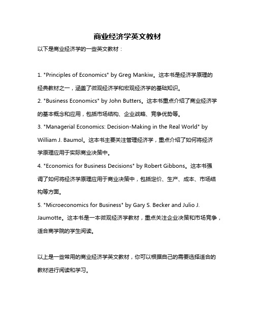
FIGURE 2.1
THE SUPPLY CURVE
The supply curve, labeled S in the figure, shows how the quantity of a good offered for sale changes as the price of the good changes. The supply curve is upward sloping: The higher the price, the more firms are able and willing to produce and sell.
• Understanding and predicting how changing world economic conditions affect market price and production
• Evaluating the impact of government price controls, minimum wages, price supports, and production incentives
• Determining how taxes, subsidies, tariffs, and import quotas affect consumers and producers
Copyright © 2013 Pearson Education, Inc. • Microeconomics • Pindyck/Rubinfeld, 8e.
When production costs decrease, output increases no matter what the market price happens to be. The entire supply curve thus shifts to the right.
Economists often use the phrase change in supply to refer to shifts in the supply curve, while reserving the phrase change in the quantity supplied to apply to movements along the supply curve.
2 of 49
2.1 Supply and Demand
The Supply Curve
● supply curve Relationship between the quantity of a good that producers are willing to sell and the price of the good.
If production costs fall, firms can produce the same quantity at a lower price or a larger quantity at the same price. The supply curve then shifts to the right (from S to S′).
2.5 Short-Run versus Long-Run Elasticities
2.6 Understanding and Predicting the Effects of Changing Market Conditions
2.7 Effects of Government Intervention—Price Controls
QS = QS(P)
Copyright © 2013 Pearson Education, Inc. • Microeconomics • Pindyck/Rubinfeld, 8e.
3 of 49
OTHER VARIABLES THAT AFFECT SUPPLY
The quantity that producers are willing to sell depends not only on the price they receive but also on their production costs, including wages, interest charges, and the costs of raw materials.
CHAPTER 2
The Basics of Supply and Demand
CHAPTERemand
2.2 The Market Mechanism
2.3 Changes in Market Equilibrium
2.4 Elasticities of Supply and Demand