Numerical modelling of the spiral plate heat exchanger

合集下载

地质与岩土工程专业英语论文tb

岩土工程英语作业姓名：汤彪学号：013621814102班级：0133018141SHORT COMMUNICATIONS ANALYTICAL METHOD FOR ANALYSIS OFSLOPE STABILITYJINGGANG CAOs AND MUSHARRAF M. ZAMAN*tSchool of Civil Engineering and Environmental Science,University of Oklahoma, Norman, OK 73019, U.S.A.SUMMARYAn analytical method is presented for analysis of slopestability involving cohesive and non-cohesive soils.Earthquakeeffects are considered in an approximate manner in terms ofseismic coe$cient-dependent forces. Two kinds of failure surfaces areconsidered in this study: a planar failure surface, and acircular failure surface. The proposed method can be viewed asan extension of the method of slices, but it provides a moreaccurate etreatment of the forces because they are representedin an integral form. The factor of safety is obtained by usingthe minimization technique rather than by a trial and errorapproach used commonly.The factors of safety obtained by the analytical method arefound to be in good agreement with those determined by the localminimum factor-of-safety, Bishop's, and the method of slices. Theproposed method is straightforward, easy to use, and lesstime-consuming in locating the most critical slip surface andcalculating the minimum factor of safety for a given slope.Copyright ( 1999) John Wiley & Sons, Ltd.Key words: analytical method; slope stability; cohesive andnon-cohesive soils; dynamic effect; planar failure surface;circular failure surface; minimization technique;factor-of-safety.INTRODUCTIONOne of the earliest analyses which is still used in manyapplications involving earth pressure was proposed by Coulomb in1773. His solution approach for earth pressures against retainingwalls used plane sliding surfaces, which was extended to analysis of slopes in 1820 by Francais. By about 1840, experience with cuttings and embankments for railways and canals in England and France began to show that many failure surfaces in clay were not plane, but signi"cantly curved. In 1916, curved failure surfaces were again reported from the failure of quay structures in Sweden. In analyzing these failures, cylindrical surfaces were used and the sliding soil mass was divided into a number of vertical slices. The procedure is still sometimes referred to as the Swedish method of slices. By mid-1950s further attention was given to the methods of analysis usingcircular and non-circular sliding surfaces . In recent years, numerical methods have also been used in the slope stability analysis with the unprecedented development of computer hardware and software. Optimization techniques were used by Nguyen,10 and Chen and Shao. While finite element analyses have great potential for modelling field conditions realistically, they usually require signi"cant e!ort and cost that may not be justi"ed in some cases.The practice of dividing a sliding mass into a number of slices is still in use, and it forms the basis of many modern analyses.1,9 However, most of these methods use the sums of the terms for all slices which make the calculations involved in slope stability analysis a repetitive and laborious process.Locating the slip surface having the lowest factor of safety is an important part of analyzing a slope stability problem. A number of computer techniques have been developed to automate as much of this process as possible. Most computer programs use systematic changes in the position of the center of the circle and the length of the radius to find the critical circle.Unless there are geological controls that constrain the slip surface to a noncircular shape, it can be assumed with a reasonablecertainty that the slip surface is circular.9 Spencer (1969) found that consideration of circular slip surfaces was as critical as logarithmic spiral slip surfaces for all practical purposes. Celestino and Duncan (1981), and Spencer (1981) found that, in analyses where the slip surface was allowed to take any shape, the critical slip surface found by the search was essentially circular. Chen (1970), Baker and Garber (1977), and Chen and Liu maintained that the critical slip surface is actually a log spiral. Chen and Liu12 developed semi-analytical solutions using variational calculus, for slope stability analysis with a logspiral failure surface in the coordinate system. Earthquake e!ects were approximated in terms of inertiaforces (vertical and horizontal) defined by the corresponding seismic coe$cients. Although this is one of the comprehensive and useful methods, use of /-coordinate system makes the solution procedure attainable but very complicated. Also, the solutions are obtained via numerical means at the end. Chen and Liu12 have listed many constraints, stemming from physical considerations that need to be taken into account when using their approach in analyzing a slope stability problem.The circular slip surfaces are employed for analysis of clayey slopes, within the framework of an analytical approach, in this study. The proposed method is more straightforward and simpler than that developed by Chen and Liu. Earthquake effects are included in the analysis in an approximate manner within the general framework of static loading. It is acknowledged that earthquake effects might be better modeled by including accumulated displacements in the analysis. The planar slip surfaces are employed for analysis of sandy slopes. A closed-form expression for the factor of safety is developed, which is diferent from that developed by Das.STABILITY ANALYSIS CONDITIONS AND SOIL STRENGTHThere are two broad classes of soils. In coarse-grained cohesionless sands and gravels, the shear strength is directly proportional to the stress level:''tan f τσθ= （1）where fτ is the shear stress at failure, /σ the effectivenormal stress at failure, and /θ the effective angle of shearing resistance of soil.In fine-grained clays and silty clays, the strength depends on changes in pore water pressures or pore water volumes which take place during shearing. Under undrained conditions, the shear strength cu is largely independent of pressure, that is u θ=0. When drainage is permitted, however, both &cohesive' and &frictional' components ''(,)c θ are observed. In this case the shear strength is given by(2)Consideration of the shear strengths of soils under drained and undrained conditions, and of the conditions that will control drainage in the field are important to include in analysis of slopes. Drained conditions are analyzed in terms of effective stresses, using values of ''(,)c θ determined from drained tests, or from undrained tests with pore pressure measurement. Performing drained triaxial tests on clays is frequently impractical because the required testing time can be too long. Direct shear tests or CU tests with pore pressure measurement are often used because the testing time is relatively shorter.Stability analysis involves solution of a problem involving force and/or moment equilibrium.The equilibrium problem can be formulated in terms of (1) total unit weights and boundary water pressure; or (2) buoyant unit weights and seepage forces. The first alternative is a better choice, because it is morestraightforward. Although it is possible, in principle, to usebuoyant unit weights and seepage forces, that procedure is fraught with conceptual diffculties.PLANAR FAILURE SURFACEFailure surfaces in homogeneous or layered non-homogeneous sandy slopes are essentially planar. In some important applications, planar slides may develop. This may happen in slope, where permeable soils such as sandy soil and gravel or some permeable soils with some cohesion yet whose shear strength is principally provided by friction exist. For cohesionless sandy soils, the planar failure surface may happen in slopes where strong planar discontinuities develop, for example in the soil beneath the ground surface in natural hillsides or in man-made cuttings.ααβ图平面破坏Figure 1 shows a typical planar failure slope. From an equilibrium consideration of the slide body ABC by a vertical resolution of forces, the vertical forces across the base of the slide body must equal to weight w. Earthquake effects may be approximated by including a horizontal acceleration kg which produces a horizontal force k= acting through the centroid of the body and neglecting vertical inertia.1 For a slice of unit thickness in the strike direction, the resolved forces of normaland tangential components N and ¹ can be written as(cos sin )N W k αα=-（3）(sin cos )T W k αα=+（4） where is the inclination of the failure surface and w is given by02(tan tan )(tan )(cot cot )2LW x x dx H x dx H γβαγαγαβ=-+-=-⎰⎰ （5） where γ is the unit weight of soil, H the height of slope, cot ,cot ,L H l H βαβ== is the inclination of the slope. Since the length of the slide surface AB is /sin cH α, the resisting force produced by cohesion is cH /sin a. The friction force produced by N is (cos sin )tan W k ααφ-. The total resisting or anti-sliding force is thus given by(cos sin )tan /sin R W k cH ααφα=-+（6）For stability, the downslope slide force ¹ must not exceed the resisting force R of the body. The factor of safety, F s , in the slope can be defined in terms of effective force by ratio R /T, that is1tan 2tan tan (sin cos )sin()s k c F k H k αφαγααβα-=+++- （7） It can be observed from equation (7) that F s is a function of a. Thus the minimum value of F s can be found using Powell's minimization technique18 from equation (7). Das reported a similar expression for F s with k =0, developed directly from equation (2) by assuming that /s f d F ττ=, where f τ is the averageshear strength of the soil, and d τ the average shear stressdeveloped along the potential failure surface.For cohesionless soils where c =0, the safety factor can bereadily written from equation (7) as 1tan tan tan s k F k αφα-=+ （8） It is obvious that the minimum value of F s occurs when a=b, and the failure becomes independent of slope height. For such cases (c=0 and k=0), the factors of safety obtainedfrom the proposed method and from Das are identical.CIRCULAR FAILURE SURFACESlides in medium-stif clays are often deep-seated, and failure takes place along curved surfaces which can be closely approximated in two dimensions by circular surfaces. Figure 2 shows a potential circular sliding surface AB in two dimensions with centre O and radius r . The first step in the analysis is to evaluate the sliding' or disturbing moment M s about the centre of thecircle O . This should include the self-weight w of the sliding mass, and other terms such as crest loadings from stockpiles or railways, and water pressures acting externally to the slope.Earthquake effects is approximated by including a horizontal acceleration kg which produces a horiazontal force k d=acting through the centroid of each slice and neglecting vertical inertia. When the soil above AB is just on the point of sliding, the average shearing resistance which is required along AB for limiting equilibrium is given by equation (2). The slide mass is divided into vertical slices, and a typical slice DEFG is shown. The self-weight of the slice is dW hdx γ=. The method assumes that the resultant forces Xl and Xr on DE and FG , respectively, are equal and opposite, and parallel to the base of the slice EF . It is realized that these assumptions are necessary to keep theanalytical solution of the slope stability problem addressed in this paper achievable and some of these assumptions would lead to restrictions in terms of applications (e.g.earth pressure on retaining walls). However, analytical solutions have a special usefulness in engineering practice, particularly in terms of obtaining approximate solutions. More rigorous methods, e.g. finite element technique, can then be used to pursue a detail solution. Bishop's rigorous method5 introduces a furthernumerical procedure to permit specialcation of interslice shear forces Xl and Xr . Since Xl and Xr are internal forces, ()l r X X -∑ must be zero for the whole section. Resolving prerpendicularly and parallel to EF , one getssin cos T hdx k hdx γαγα=+（9）cos csin N hdx k hdx γαγα=-（10）22arcsin ,x a r a b rα-==+ （11）The force N can produce a maximum shearing resistance when failure occurs:sec (cos sin )tan R cdx hdx k αγααφ=+-（12）The equations of lines AC , CB , and AB Y are given by y22123tan ,,()y x y h y b r x a β===---（13）The sums of the disturbing and resisting moments for all slices can be written as013230(sin cos )()(sin cos )()(sin cos )()ls l lL s c M r h k dx r y y k dx r y y k dx r I kI γααγααγααγ=+=-++-+=+⎰⎰⎰ (14) []02300232sec (cos sin )tan sec ()(cos sin )tan ()(cos sin )tan tan ()lr l l lL c s M r c h k dx r c dx r y y k dx r y y k dx r c r I kI αγααφαγααφγααφϕγφ=+-=+--+--=+-⎰⎰⎰⎰ (15)22cot ,()L H l a r b H β==+-- （16）arcsinarcsin l a a r r ϕ-=+ （17） 1323022()sin ()sin 1(cot )sec 23Ll s L I y y dx y y dxH a b H rααββ=-+-⎡⎤=+-⎢⎥⎣⎦⎰⎰ （18） 13230222222222()cos ()cos tan tan 2()()()623(tan )arcsin (tan )arcsin 221()arcsin()4()()26L l s L I y y dx y y dxb r b r L a r L a r r r L a r a a H a b r r r l a b H r l ab l a H a r r ααββββ=-+-⎡⎤=-+---++⎣⎦-⎛⎫⎛⎫+-+- ⎪ ⎪⎝⎭⎝⎭-⎡⎤--+-+--⎣⎦⎰⎰ （19） The safety factor for this case is usually expressed as the ratio of the maximum available resisting moment to the disturbing moment, that istan ()()c s r s s s c c r I kI M F M I kI ϕγφγ+-==+ (20) When the slope inclination exceeds 543, all failures emerge at the toe of the slope, which is called t oe failure , as shown in Figure 2. However, when the slope height H is relatively large compared with the undrained shear strength or when a hard stratum is under the top of the slope of clayey soil with 03φ<, the slide emerges from the face of the slope, which is called Face failure , as shown in Figure 3. For Face failure , the safety factor F s is the same as ¹oe failure 1s using 0()Hh - instead of H .For flatter slopes, failure is deep-seated and extends to the hard stratum forming the base of the clay layer, which is called Base failure , as shown in Figure 4.1,3 Following the sameprocedure as that for ¹oe failure , one can get the safety factor for Base failure :()''''tan ()c s s s c c r I kI F I kI ϕγφγ+-=+ （21） where t is given by equation (17), and 's I and 'c I are given by()()()0100'0313230322201sin sin sin cot ()()(2)(33)12223l l l s l l I y y xdx y y xdx y y xdx H H bl H l l l l l a b bH H r r r β=-+-+-=+----+-+⎰⎰⎰ (22)()()()()()()[]22222203231030c 4612cot arcsin 2tan arcsin 21arcsin 2cot 412cos cos cos 1100a H a l ab l r r r H H a r r a rb r a H b r H r r Hl d y y d y y d y y I x l l x l l x l --+-+⎪⎭⎫ ⎝⎛⎪⎭⎫ ⎝⎛-+⎪⎭⎫ ⎝⎛-⎪⎭⎫ ⎝⎛----=⎰-+⎰-+⎰-='βββααα（23）其中，()221230,tan ,,y y x y H y b r x a β====---（24） ()220111cot ,cot ,22l a H l a H l a r b H ββ=-=+=+--(25)It can be observed from equations (21)~(25) that the factor of safety F s for a given slope is a function of the parameters a and b. Thus, the minimum value of F s can be found using the Powell's minimization technique.For a given single function f which depends on two independent variables, such as the problem under consideration here, minimization techniques are needed to find the value of these variables where f takes on a minimum value, and then to calculate the corresponding value of f. If one starts at a point P in an N-dimensional space, and proceed from there in some vector direction n, then any function of N variables f (P) can be minimized along the line n by one-dimensional methods. Different methods will difer only by how, at each stage, they choose the next direction n. Powell "rst discovered a direction set method which produces N mutually conjugate directions.Unfortunately, a problem of linear dependence was observed in Powell's algorithm. The modiffed Powell's method avoids a buildup of linear dependence.The closed-form slope stability equation (21) allows the application of an optimization technique to locate the center of the sliding circle (a, b). The minimum factor of safety Fs min then obtained by substituting the values of these parameters into equations (22)~(25) and the results into equation (21), for a base failure problem (Figure 4). While using the Powell's method, the key is to specify some initial values of a and b. Well-assumed initial values of a and b can result in a quick convergence. If the values of a and b are given inappropriately, it may result in a delayed convergence and certain values would not produce a convergent solution. Generally, a should be assumed within$¸, while b should be equal to or greater than H (Figure 4). Similarly, equations(16)~(20) could be used to compute the F s .min for toe failure (Figure 2) and face failure (Figure 3),except ()0H h - is usedinstead of H in the case of face failure .Besides the Powell method, other available minimization methods were also tried in this study such as downhill simplex method, conjugate gradient methods, and variable metric methods. These methods need more rigorous or closer initial values of a and b to the target values than the Powell method. A short computer program was developed using the Powell method to locate the center of the sliding circle (a , b ) and to find the minimum value of F s . This approach of slope stability analysis is straightforward and simple.RESULTS AND COMMENTSThe validity of the analytical method presented in the preceding sections was evaluated using two well-established methods of slope stability analysis. The local minimumfactor-of-safety (1993) method, with the state of the effective stresses in a slope determined by the finite element method with the Drucker-Prager non-linear stress-strain relationship, and Bishop's (1952) method were used to compare the overall factors of safety with respect to the slip surface determined by the proposed analytical method. Assuming k =0 for comparison with the results obtained from the local minimum factor-of-safety and Bishop's method, the results obtained from each of those three methods are listed in Table I.The cases are chosen from the toe failure in a hypothetical homogeneous dry soil slope having a unit weight of 18.5 kN/m3. Two slope configurations were analysed, one 1 : 1 slope and one 2 : 1 slope. Each slope height H was arbitrarily chosen as 8 m. To evaluate the sensitivity of strength parameters on slope stability, cohesion ranging from 5 to 30 kPa and friction angles ranging from 103 to 203 were used in the analyses (Table I). Anumber of critical combinations of c and were found to be unstable for the model slopes studied. The factors of safety obtained by the proposed method are in good agreement with those determined by the local minimum factor-of-safety and Bishop's methods, as shown in Table I.To examine the e!ect of dynamic forces, the analytical method is chosen to analyse a toe failure in a homogeneous clayey slope (Figure 2). The height of the slope H is 13.5 m; the slope inclination b is arctan 1/2; the unit weight of the soil c is 17.3 kN/m3; the friction angle is 17.3KN/m; and the cohesion c is 57.5 kPa. Using the conventional method of slices, Liu obtained theminimum safety factormin 2.09sF= Using the proposed method, one can get the minimum value of safety factor from equation (20) asmin 2.08sF= for k=0, which is very close to the value obtained from the slice method. When k"0)1, 0)15, or 0)2, one cangetmin 1.55,1.37sF=, and 1)23, respectively,which shows the dynamic e!ect on the slope stability to be significant.CONCLUDING REMARKSAn analytical method is presented for analysis of slope stability involving cohesive and noncohesive soils. Earthquake e!ects are considered in an approximate manner in terms of seismic coe$cient-dependent forces. Two kinds of failure surfaces are considered in this study: a planar failure surface, and a circular failure surface. Three failure conditions for circular failure surfacesnamely toe failure, face failure, and base failure are considered for clayey slopes resting on a hard stratum.The proposed method can be viewed as an extension of the method of slices, but it provides a more accurate treatment of the forces because they are represented in an integral form. The factor of safety is obtained by using theminimization technique rather than by a trial and error approach used commonly.The factors of safety obtained from the proposed method are in good agreement with those determined by the local minimum factor-of-safety method (finite element method-based approach), the Bishop method, and the method of slices. A comparison of these methods shows that the proposed analytical approach is more straightforward, less time-consuming, and simple to use. The analytical solutions presented here may be found useful for (a)validating results obtained from other approaches, (b) providinginitial estimates for slope stability, and (c) conducting parametric sensitivity analyses for various geometric and soil conditions.REFERENCES1. D. Brunsden and D. B. Prior. Slope Instability, Wiley, New York, 1984.2. B. F. Walker and R. Fell. Soil Slope Instability and Stabilization, Rotterdam, Sydney, 1987.3. C. Y. Liu. Soil Mechanics, China Railway Press, Beijing, P. R. China, 1990.448 SHORT COMMUNICATIONSCopyright ( 1999 John Wiley & Sons, Ltd. Int. J. Numer. Anal. Meth. Geomech., 23, 439}449 (1999)4. L. W. Abramson. Slope Stability and Stabilization Methods, Wiley, New York, 1996.5. A. W. Bishop. &The use of the slip circle in the stability analysis of slopes', Geotechnique, 5, 7}17 (1955).6. K. E. Petterson. &The early history of circular sliding surfaces', Geotechnique, 5, 275}296 (1956).7. G. Lefebvre, J. M. Duncan and E. L. Wilson.&Three-dimensional "nite element analysis of dams,' J. Soil Mech. Found,ASCE, 99(7), 495}507 (1973).8. Y. Kohgo and T. Yamashita, &Finite element analysis of "ll type dams*stability during construction by using the e!ective stress concept', Proc. Conf. Numer. Meth. in Geomech., ASCE, Vol. 98(7), 1998, pp. 653}665.9. J. M. Duncan. &State of the art: limit equilibrium and "nite-element analysis of slopes', J. Geotech. Engng. ASCE, 122(7), 577}596 (1996).10. V. U. Nguyen. &Determination of critical slope failuresurface', J. Geotech. Engng. ASCE, 111(2), 238}250 (1985).11. Z. Chen and C. Shao. &Evaluation of minimum factor of safety in slope stability analysis,' Can. Geotech. J., 20(1), 104}119 (1988).12. W. F. Chen and X. L. Liu. ¸imit Analysis in Soil Mechanics, Elsevier, New York, 1990.简要的分析斜坡稳定性的方法JINGGANG CAOs 和 MUSHARRAF M. ZAMAN诺曼底的俄克拉荷马大学土木环境工程学院摘要本文给出了解析法对边坡的稳定性分析,包括粘性和混凝土支撑。

Mathematical Modelling and Numerical Analysis Will be set by the publisher Modelisation Mat

& luskin@
c EDP Sciences, SMAI 1999
2

PAVEL BEL K AND MITCHELL LUSKIN
In general, the analysis of stability is more di cult for transformations with N = 4 such as the tetragonal to monoclinic transformations studied in this paper and N = 6 since the additional wells give the crystal more freedom to deform without the cost of additional energy. In fact, we show here that there are special lattice constants for which the simply laminated microstructure for the tetragonal to monoclinic transformation is not stable. The stability theory can also be used to analyze laminates with varying volume fraction 24 and conforming and nonconforming nite element approximations 25, 27 . We also note that the stability theory was used to analyze the microstructure in ferromagnetic crystals 29 . Related results on the numerical analysis of nonconvex variational problems can be found, for example, in 7 12,14 16,18,19,22,26,30 33 . We give an analysis in this paper of the stability of a laminated microstructure with in nitesimal length scale that oscillates between two compatible variants. We show that for any other deformation satisfying the same boundary conditions as the laminate, we can bound the pertubation of the volume fractions of the variants by the pertubation of the bulk energy. This implies that the volume fractions of the variants for a deformation are close to the volume fractions of the laminate if the bulk energy of the deformation is close to the bulk energy of the laminate. This concept of stability can be applied directly to obtain results on the convergence of nite element approximations and guarantees that any nite element solution with su ciently small bulk energy gives reliable approximations of the stable quantities such as volume fraction. In Section 2, we describe the geometrically nonlinear theory of martensite. We refer the reader to 2,3 and to the introductory article 28 for a more detailed discussion of the geometrically nonlinear theory of martensite. We review the results given in 34, 35 on the transformation strains and possible interfaces for tetragonal to monoclinic transformations corresponding to the shearing of the square and rectangular faces, and we then give the transformation strain and possible interfaces corresponding to the shearing of the plane orthogonal to a diagonal in the square base. In Section 3, we give the main results of this paper which give bounds on the volume fraction of the crystal in which the deformation gradient is in energy wells that are not used in the laminate. These estimates are used in Section 4 to establish a series of error bounds in terms of the elastic energy of deformations for the L2 approximation of the directional derivative of the limiting macroscopic deformation in any direction tangential to the parallel layers of the laminate, for the L2 approximation of the limiting macroscopic deformation, for the approximation of volume fractions of the participating martensitic variants, and for the approximation of nonlinear integrals of deformation gradients. Finally, in Section 5 we give an application of the stability theory to the nite element approximation of the simply laminated microstructure.

高二英语数学建模方法单选题20题

高二英语数学建模方法单选题20题1.In the process of mathematical modeling, the factor that determines the outcome is called_____.A.independent variableB.dependent variableC.control variableD.extraneous variable答案：B。

本题考查数学建模中的基本术语。

独立变量（independent variable）是指在实验或研究中被研究者主动操纵的变量；因变量dependent variable）是指随着独立变量的变化而变化的变量，在数学建模中决定结果的因素通常是因变量；控制变量（control variable）是指在实验中保持不变的变量；无关变量（extraneous variable）是指与研究目的无关，但可能会影响研究结果的变量。

2.The statement “The value of y depends on the value of x” can be represented by a mathematical model where y is the_____.A.independent variableB.dependent variableC.control variableD.extraneous variable答案：B。

在“y 的值取决于x 的值”这句话中，y 是随着x 的变化而变化的变量，所以y 是因变量。

3.In a mathematical model, the variable that is held constant toobserve the effect on other variables is_____.A.independent variableB.dependent variableC.control variableD.extraneous variable答案：C。

Numerical modeling of the microstructure of carbon-carbon composites on different length scales

ineering Mechanics, University of Karlsruhe (TH), Kaiserstraße 10, D-76131 Karlsruhe (Germany) Department of Mechanical Engineering, University of New Hampshire, Durham, NH 03824 (USA) 3 Institute of Chemical Technology and Polymer Chemistry, University of Karlsruhe (TH), Engesserstraße 20, D-76131 Karlsruhe (Germany) 4 Nuclear Research Centre Negev, P.O. Box 9001, Beer-Sheva, 84190 (Israel)
2
* Corresponding author. E-mail: romana.piat@ Abstract. Carbon/carbon composites produced by chemical vapour infiltration consist of carbon fibers embedded in a matrix of pyrolytic carbon with anisotropic mechanical properties. Microscopic studies show that the production process facilitates formation of a matrix consisting of cylindrically shaped pyrolytic carbon layers. The matrix layers may have different textures, which induce different mechanical properties in the axial, radial and circumferential directions. By modifying the production process parameters, it is possible to control the order, approximate width and degree of texture of the layers. Depending on the infiltration conditions pores with different geometry, size and orientations are formed between fibers with pyrolytic carbon coating. One of the goals of the present study is the microstructure characterization and the statistical description of the matrix texture, the fibers orientation distribution and the porosity. Furthermore, a micromechanical modeling using homogenization methods of the material on different length scales is performed. Correlation between calculated and experimentally obtained material properties is also discussed.

英文文献

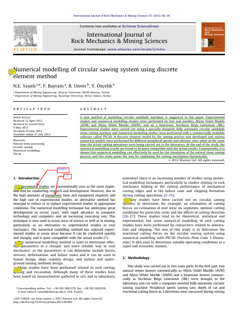
modelling of circular sawing system using discretemethodN.E.Yas-ıtlıa,n,F.Bayram a,B.Unver b,Y.O¨zc-elik ba Department of Mining Engineering,Aksaray University,68100Aksaray,Turkeyb Department of Mining Engineering,Hacettepe University,06532Ankara,Turkeya r t i c l e i n f oArticle history:Received12April2011Received in revised form9May2012Accepted19June2012Available online21July2012Keywords:Natural stone processingCircular sawingNumerical modellingPFC3Da b s t r a c tA new method of modelling circular sawblade machines is suggested in this paper.Experimentalstudies and numerical modelling studies were performed on two real marbles,Afyon Violet Marble(AVM)and Afyon White Marble(AWM),and on a limestone,Sivrihisar Beige Limestone(SBL).Experimental studies were carried out using a specially designed,fully automatic circular sawbladestone cutting machine and numerical modelling studies were performed with a commercially availablesoftware called PFC3D.A discrete element model for the sawing process was developed and variousnumerical models were performed for different peripheral speeds and advance rates while at the sametime the actual cutting operations were being carried out in the laboratory.At the end of the study,thenumerical modelling results are found to be quite compatible with the actual results.Consequently,it isshown that numerical modelling can effectively be used for the simulation of the natural stone sawingprocess,and this study paves the way for explaining the sawing mechanism dynamically.&2012Elsevier Ltd.All rights reserved.seen as the most impor-However,due tomanpower,equipment required,andthe high cost of experimental studies,an alternative method hasemerged to reduce or to replace experimental studies in appropriateconditions.The numerical modelling technique has undergone greatdevelopment in recent years,with rapid advances in computertechnology and computers and an increasing executing rate.Thistechnique is now used in many areas of science as well as in mining,particularly as an alternative to experimental studies in rockmechanics.The numerical modelling method has replaced experi-mental studies in many areas because it can be conducted quicklyand cheaply,and is quite compatible with the actual results[1].numerical modelling method is used to determine effec-in a cheaper and more reliable way in rockmechanics;as the parameters it can determine include forces,stresses,deformations and failure zones and it can be used intunnel design,slope stability design,and surface and under-ground mining methods design.studies have been performed related to rock cutting,and excavation.Although many of these studies havebeen based on measurements gathered in situ and in laboratory,nowadays there is an increasing number of studies using numer-ical modelling techniques,particularly in studies relating to rockmechanics looking at the cutting performance of mechanicalcutting edges and at the failure zone and chipping formationcutting operations[2–15].studies have been carried out on circular sawingto determine,for example,an estimation of cuttingforces,an estimation of unit wear on segments,optimal cuttingconditions for particular rocks and the effects of cutting direction[16–27].These studies tend to be theoretical,statistical andexperimental,but some numerical modelling of rock cuttingstudies have been performed by researchers related to indenta-tion and chipping.The aim of this study is to determine thereactional cutting forces on the circular sawing system usingnumerical modelling with PFC3D(Particle Flow Code3Dimen-sion).It also aims to determine suitable operating conditions in arapid and economic manner.2.MethodologyThis study was carried out in two main parts.In theﬁrst part,twonatural stones known commercially as Afyon Violet Marble(AVM)and Afyon White Marble(AWM)and a limestone known commer-cially as Sivrihisar Beige Limestone(SBL)were brought to thelaboratory and cut with a computer-assisted fully-automatic circularsawing machine.Peripheral speed,sawing rate,depth of cut andreactional cutting forces in3directions were measured during sawingContents lists available at SciVerse ScienceDirectjournal homepage:/locate/ijrmmsInternational Journal ofRock Mechanics&Mining Sciences1365-1609/$-see front matter&2012Elsevier Ltd.All rights reserved./10.1016/j.ijrmms.2012.06.006n Corresponding author.Tel.:þ903822882379;fax:þ903822802298.E-mail address:eyasitli@.tr(N.E.Yas-ıtlı).International Journal of Rock Mechanics&Mining Sciences55(2012)86–96operations by means of load cells,sensors and an analyser mounted on the circular sawing machine.In the second part,numerical modelling of the circular sawing mechanism was performed.The parameters taken from at theﬁrst part were used as input parameters to the numerical model.The model was created in PFC3D,then the assignment of required data was done and numerical modelling of sawing was performed.Finally,the laboratory results were compared with the results obtained from modelling.3.Experimental studies and circular sawing operationsThe experimental study was conducted in three stages.In theﬁrst stage,the real marble samples AVM and AWM,and the limestone SBL were prepared to dimensions of200Â300Â500mm3.In the second stage,the rock mechanics tests were performed in order to determine the physical and mechanical properties of the natural stones.The results of these tests are given in Table1.In the third stage,the sawing operations were carried out at different peripheral speeds and advance rates.puter-assisted fully-automatic circular sawing machineA computer-assisted fully automatic circular sawing machine was designed and the machine parameters that are effective during the sawing process,such as the effective forces in the X, Y and Z directions,were identiﬁed,and the controlling sawing conditions(sawing rate,peripheral speed of the saw,sawing depth,etc)were provided[28].Due to a special platform located on the top of the wagon,the three-dimensional reactional forces that occur during the sawing process could be measured by load cells.In order to identify the horizontal reactional forces(X and Y)on this platform,two load cells are used for each direction,which,together with the three load cells used to identify the vertical reactional force(Z),gives a total of seven load cells.The four load cells used for the identiﬁcation of the horizontal reactional forces are Flintec types, UB6code,with a capacity of100kg(tension type),and the three load cells used for the identiﬁcation of the vertical reactional forces are also Flintec types,SB14code,with a capacity of200kg (beam type).The load cells are able to measure to70.01kg sensitivity.The fully-automatic circular sawing machine can be controlled either manually or by computer.An automation programme was developed to convey the necessary parameters(advance rate, peripheral speed,sawing depth,sawing width,number of saw-ings,etc)to the machine via computer during the sawing,and to monitor and record the three-dimensional reactional sawing force data that occur during sawing.3.2.Sawing operationsThe sawing operations were performed under24sawing conditions at four different peripheral speeds(40–70m/s)and six different advance rates(400–900mm/min)for each natural stone with the saw at a constant depth of60mm.For each sawing condition,the sawing operations were repeated5times.During the sawing operations,some data,such as height of sample,depth of cut,peripheral speed and advance rate,were entered into the software that controlled the machine;then the sawing was carried out in the form of a channel and was repeatedﬁve times.After the sawing operation,four data per second obtained from the load cells were recorded on a computer.The horizontal and vertical reactional forces that occurred during this sawing operation can be seen in Fig.1.At the end of the sawing operations,it was found that the reactional forces did not show a regular trend in the horizontal directions(X and Y);therefore,the analysis of these forces was not taken into account.In this study,only the vertical forces that occurred in the Z direction were examined in detail.With the start of the sawing operation in Region I,the sawblade is in contact with the block and the reactional cutting forces begin.Maximum contact between the block and the sawblade occurs in Region II,where the vertical reactional cutting forces reach their maximum values.The vertical reactional cut-ting forces remain at approximately the same level in Region II. With the sawblade leaving the block in Region III,the reactional cutting forces reduce suddenly.Due to the minimal contact between the block and the sawblade,the reactional cutting forces remain at approximately at the same level.When the whole sawblade leaves the block,the sawing operation stops;conse-quently,recording of the data also stops.The blocks used in the laboratory are500mm in length.How-ever,this would be much longer in plant.Therefore,in order to apply the results of this study to a plant scale,the reactional cutting forces obtained from sawing operation were evaluated for the whole line(the total of Regions I,II and III)and for just the middle region (Region II)separately,and the analysis was carried out in this scope.3.2.1.Reactional cutting forces for different peripheral speedsThe averages of the vertical reactional forces obtained for the whole cutting line and for the middle region at40m/s peripheral speed are presented graphically in Fig.2for AVM.The average vertical reactional forces along the whole line and middle region for the lowest advance rate of400mm/min are63.43N and 117.68N,respectively.For the highest advance rate of900mm/ min,the average vertical reactional forces for whole line and for middle region are176.4N and374.16N,respectively.The average vertical reactional forces between400mm/min and900mm/min change in these values.As seen in Fig.2,the reactional forces increase linearly as the advance rate increases.From the results,it can be seen that the vertical reactional cutting forces have values approximately twice as high in the cases where the advance rate is at its lowest than where it is at its highest at constant peripheral speeds.The reason why the reactional cutting force increases as the advance rate increases at a constant peripheral speed is that the amount of material that will be cut in a unit of time,or,in other words,the sawblade’s amount of contact with the block in a speciﬁc unit ofTable1Physical and mechanical properties of the natural stones.Sample Natural Stone Lithologic UVW WA P UCS E UTS H S No Trade Name Name(gr/cm3)(%)(%)(MPa)(GPa)(MPa)–1Afyon Violet Real Marble 2.670.060.1573.9417.6 5.4942 2Afyon White Real Marble 2.650.050.1551.4515.5 6.2249 3Sivrihisar Beige Limestone 2.700.120.2270.0022.27.0562UVW:unit volume weight,WA:water absorption,P:porosity,UCS:uniaxial compressive strength,E:elasticity modulus,UTS:uniaxial tensile strength,H S:shore scleroscope hardness.N.E.Yas-ıtlıet al./International Journal of Rock Mechanics&Mining Sciences55(2012)86–9687time,increases,and,therefore,the cutting force increases.Conversely,at a constant advance rate,since the peripheral speed increases as the sawblade’s contact with the block in any unit of time decreases,the cutting force decreases.As a result of the sawing operation for AVM,linear relationships are obtained with R 2¼0.945–0.987for the whole cutting line and R 2¼0.903–0.979Fig.1.Reactional forces in three directions during sawing.I.Region:Sawing starts and sawblade enters the block with the wagon advancing,II.Region:Whole sawblade isin the block and contact between the block and the saw is at its maximum and III Region:The sawblade starts to leave the block and the whole sawblade is out of the block as the wagon advances.050100150200250300050100150200250300350400Peripheral Speed : 40 m/sPeripheral Speed : 50 m/sPeripheral Speed : 60 m/sPeripheral Speed : 70 m/sAdvance Speed (mm/min)V e r t i c a l R e a c t i o n a l C u t t i n g F o r c e (N )V e r t i c a l R e a c t i o n a l C u t t i n g F o r c e (N )V e r t i c a l R e a c t i o n a l C u t t i n g F o r c e (N )V e r t i c a l R e a c t i o n a l C u t t i n g F o r c e (N )2004006008001000Advance Speed (mm/min)2004006008001000Advance Speed (mm/min)2004006008001000Advance Speed (mm/min)2004006008001000Fig.2.Average of the vertical reactional forces occurring in the whole cutting line and in the central region for AVM.N.E.Yas -ıtlıet al./International Journal of Rock Mechanics &Mining Sciences 55(2012)86–968850100150200250050100150200250300350050100150200250300Peripheral Speed : 40 m/sPeripheral Speed : 50 m/sPeripheral Speed : 60 m/sPeripheral Speed : 70 m/sAdvance Speed (mm/min)V e r t i c a l R e a c t i o n a l C u t t i n g F o r c e (N )V e r t i c a l R e a c t i o n a l C u t t i n gF o r c e (N )V e r t i c a l R e a c t i o n a l C u t t i n g F o r c e (N )V e r t i c a l R e a c t i o n a l C u t t i n g F o r c e (N )Advance Speed (mm/min)Advance Speed (mm/min)Advance Speed (mm/min)Fig.3.Average of vertical reactional forces occurring in whole cutting line and in the central region for AWM.050100150200250300350400450050100150200250300350050100150200250300350050100150200250300Peripheral Speed : 40 m/sPeripheral Speed : 50 m/sPeripheral Speed : 60 m/sPeripheral Speed : 70 m/s Advance Speed (mm/min)V e r t i c a l R e a c t i o n a l C u t t i n g F o r c e (N )V e r t i c a l R e a c t i o n a l C u t t i n g F o r c e (N )V e r t i c a l R e a c t i o n a l C u t t i n g F o r c e (N )V e r t i c a l R e a c t i o n a l C u t t i n g F o r c e (N )Advance Speed (mm/min)0Advance Speed (mm/min)2004006008001000Advance Speed (mm/min)Fig.4.Average of vertical reactional forces occurring in whole cutting line and in the central region for SBL.N.E.Yas -ıtlıet al./International Journal of Rock Mechanics &Mining Sciences 55(2012)86–9689for the middle region.The same process was carried out for AWM and SBL(Figs.3and4)and it was found that for AWM R2¼0.939–0.990for the whole cutting line and R2¼0.964–0.991 for the middle region,while for SBL R2¼0.989–0.997for the whole cutting line and R2¼0.903–0.979for the middle region. 4.Numerical modelling studiesNumerical modelling studies were carried out using a com-mercially available software called PFC3D,which was developed by Itasca Consulting,and which works on the principle of distinct element modelling.4.1.Distinct element method and numerical modelling softwareof PFC3DThe distinct element method(DEM)is a numerical method which models solid objects using round,spherical and polygon-shaped particles.The basic approach and analysis of DEM was ﬁrst developed by Cundall[29].It has been used in various disciplines for modelling micro-and macro-sized materials[30]. The most commonly known and used DEM programs are UDEC, 3DEC,PFC2D,PFC3D and DDA[31–33].DEM allowsﬁnite displacements and rotations of discrete bodies,including complete detachment,and recognises new contacts automatically during the calculation processes.In DEM, the interactions between the particles are treated as a dynamic process with states of equilibrium developing whenever the internal forces balance.The calculations performed in the DEM alternate between the application of Newton’s second law to the particles and a force-displacement law at the contacts.PFC3D is a three-dimensional numerical modelling pro-gramme that analyses the interactions of objects with each other using spherical particles.It models the mechanical behaviours of the objects according to dynamic behaviour.While the behaviour of the particles is determined using Newton’s Law of Movement as the basis,the interactions among particles are deﬁned using contact models.The contact model in PFC3D is a soft contact method,which allows very little overlapping in a fairly small area.Particles must be in contact with each other in modelling studies performed in theﬁeld of rock mechanics.Contact models known as the Bonded Particle Model(BPM)are used among the particles.BPM provides both a scientiﬁc tool to investigate the micromechanisms that combine to produce complex macroscopic behaviours and an engineering tool to predict these macroscopic behaviours[34].The emergence,development and interaction of microcracks affect the mechanical behaviours of rocks.Therefore, BPM is used to model the mechanical behaviours of the spherical particles of both regular and irregular sizes that are bonded to each other from a contact point.The term particle,as used here, has a different meaning to its more common deﬁnition in theﬁeld of mechanics;here it means a body whose dimensions are negligible and that,therefore,occupies only a single point in space.Solid particles affect each other only by thin contact and they haveﬁnite normal and shear stiffnesses.The normal stiff-ness,K n,is a secant modulus in that it relates to total displace-ment and force.The shear stiffness,k s,on the other hand,is a tangent modulus in that it relates to incremental displacement and force(Eq.(1)).An upper-case K will be used to denote a secant modulus,and a lower-case k will be used to denote a tangent modulus.The mechanical behaviour of this system is deﬁned by the movement of each particle,force and moment affected at each contact.Newton’s Law of Motion provides the basic relationships between the force arising as a result of a particle’s movement and moments[34]:F i¼F niþF sið1ÞF ni¼K n U n n ið2ÞD F si¼Àk s D U s ið3ÞThere are two types of elements deﬁned in PFC3D:particle and wall elements.The wall in the programme forms a solid object that keeps the particles together at the beginning of the model.In this study,particles are located inside a cube formed by the wall elements.Moreover,a circular wall representing the sawblade is also used in the modelling study.In PFC3D,particles interact both with each other and with the wall.4.2.Parallel bonded modelNumerical modelling studies have been carried out using contact models,including in PFC3D.Although there are a lot of models in PFC3D,the Parallel Bonded Model(PBM)was chosen in order to deﬁne and model connected materials with each other.The PBM describes the constitutive behaviour of aﬁnite-sized piece of cementatious material deposited between two particles. These bonds establish an elastic interaction between particles. Thus,the existence of a parallel bond does not preclude the possibility of slip.Parallel bonds can transmit both forces and moments between particles.Thus,parallel bonds may contribute to the resultant force and moment acting on two bonded particles.Relative motion at the point of contact(occurring after the parallel bond has been created)causes a force and a moment to develop within the bond material as a result of the parallel-bond stiffnesses.This force and moment act on the two bonded particles and can be related to maximum normal and shear stresses acting within the bond material at the bond periphery.A parallel bond is deﬁned by the followingﬁve parameters: normal and shear stiffness n and s(stress/displacement); normal and shear strength s c and t c;and bond disc radius R. These parameters are speciﬁed by the pb_kn,pb_ks,pb_n strength, pb_s strength and pb_radius keywords.If the maximum tensile stress exceeds the normal strength(s max Z s c)or the maximum shear stress exceeds the shear strength(t max Z t c),then the parallel bond breaks.4.3.Calibration of micromechanical parameters of rock specimensThe discrete element model can be regarded as micromecha-nical material model,with the contact model parameters being micromechanical parameters.Assuming adequate micromecha-nical parameters the required macroscopic rock properties can be obtained.The most important macroscopic rock properties include;the Elasticity modulus(E),Poisson’s ratio(n),uniaxial compressive strength(UCS)and uniaxial tensile strength(UTS). These properties were used in calibrating the micromechanical model used in this work.The discrete element model can also be calibrated using other macroscopic rock properties such as the shear strength,the angle of internal friction or fracture toughness [35,15,36].For this purpose,as seen in Fig.5,prismatic and cylindrical specimens were created according to the procedure mentioned in the PFC3D manual[30].Since it is very difﬁcult to determine microscopic properties at particle level by experimen-tal measurements,it is essential to establish a correlation between the properties of the bulk materials and the properties at the particle level to validate the particle properties used in the modelling.During the calibration process,the micro-properties were varied systematically using the trial and error method.The axial stress versus the axial strain,and the axial stress versusN.E.Yas-ıtlıet al./International Journal of Rock Mechanics&Mining Sciences55(2012)86–96 90lateral strain curves were plotted after each trial and checked toascertain whether the curves exhibit the macro-properties.This process was repeated until the response of the model achieved a good agreement with the response of the rock sample.On completion of the calibration,the laboratory and simulation results were matched.The calibration results after modelling of E ,UCS ,UTS and Poisson’s ratio test are given in Table 2.In addition,in order to realistically represent circular sawing,the appropriate particle radii should be determined.During the calibration studies the particle radius was also changed usingthe trial and error method and for the sawing modelling the particle radius was found to be 1.5mm [37].The BPM parameters at particle level used for the numerical tests,listed in Table 3,could be introduced in the subsequent modelling of circular sawing.4.4.Constitution of the modelsThe numerical modelling of sawing operation in PFC3D consists of seven parts:determination of the restrictions,deter-mination of the material properties,formation of the model geometry and particles,deﬁnition of the relations between particles,determination of the boundary and initial conditions,initial running of the programme and monitoring of the responses of the model,re-evaluation of the model and undertaking any necessary modiﬁcations,and obtaining the results.The determination of the restrictions and the material proper-ties refers to the assumptions made during the numerical studies implemented with PFC3D.One restriction was to deﬁne appro-priate sawblade properties.The circular sawblade placed on the model was deﬁned as being of very strong material behaving as a rigid cutting tool.The material properties for each natural stone sample to be entered into the programme were determined during the calibration of the micromechanical parameters.By forming the model’s geometry and particles,the shape of the model and the desired size of particles can be explained.The procedure for the deﬁnition of the relationships between particles means entering the bonding properties of the particles into the model in order to observe the interactions between the particles that have bonded or after bond breakage.These are the fundamental actions to constitute the model.After this process,the system will be modelled but further procedures still need to be undertaken.First of all,the installation of the sawblade and deﬁnition of the cutting condition such as different peripheral speed and advance rate of the sawblade was expressed as boundary and initial conditions should be entered into the model at boundaries.After these processes,the model will be run and the results willbeFig.5.General procedure for calibration of micromechanical properties of rock specimens.Table 2Main mechanical properties of rock specimens in the macro-test and DEM.Mechanical propertiesAVMAWMSBLExperiment resultsDEM model results Experiment results DEM model results Experiment results DEM model results UCS s c (MPa)73.9472.9251.4547.9270.0072.88Elasticity modulus E (GPa)17.6016.6815.5017.4022.2023.30Poisson’s ratio n 0.240.240.230.230.240.24UTS s t (MPa)5.499.996.225.537.056.74Table 3DEM parameters for rock specimens.AVM AWM SBL ParticlesParallel bondParticlesParallel bondParticlesParallel bondr ¼2.67g/cm 3l ¼1r ¼2.65g/cm 3l _¼1r ¼2.70g/cm 3l _¼1k n /k s ¼2.5n =s ¼2.5k n /k s ¼2.5n =s ¼2.5k n /k s ¼2.5n =s ¼2.5E c ¼18.9GPac ¼18.9GPaE c ¼17.0GPac ¼17.0GPa E c ¼23.0GPaE c _¼23.0GPa R max /R min ¼1R min ¼1.5mm s n _¼62712MPa R max /R min ¼1R min ¼1.5mm s n ¼3977MPa R max /R min ¼1R min ¼1.5mms n _¼60712MPa m ¼0.5s s _¼62712MPam ¼0.5s s ¼3977MPam ¼0.5s s _¼60712MPar density of the particles,k n /k s ratio of normal to shear stiffness of the particles,E c Elasticity modulus of the particles,R max /R min ratio of particles’maximum radius to minimum radius,m friction factor,l radius multiplier of the parallel-bond,n =s ratio of normal to shear stiffness of the parallel bond,s n tensile strength of the parallel-bond,s s shear strength of the parallel-bond.N.E.Yas -ıtlıet al./International Journal of Rock Mechanics &Mining Sciences 55(2012)86–9691investigated.If there is an error,the source of the problem will befound and the necessary changes can be made.4.5.Model geometry and particle assignmentAs a result of the calibration of micromechanical parameters,the appropriate particle size was found to be a 1.5mm radius,and so this was used during sawing modelling.The length of the marble block cut in numerical modelling was taken as 300mm.The depth of cut was taken as 60mm and the block height chosen was 100mm.The model width was selected as 6mm to comply with the segment width (5.6mm)and the channel width (6mm)formed during cutting.The model is surrounded by an element deﬁned as a wall in the PFC3D programme.In order to determine the reactional cutting force at the bottom of the model,29measurement spheres were located (Fig.6).Various parameters within a PFC3D model can be measured over a given spherical volume.The user speciﬁes the location and size of the measurement sphere.These spheres can be deﬁned to measure porosity,stress,strain rate,coordination number and force.A circular wall of 500mm diameter was located in the model to represent the circular sawblade (Fig.6).During the calculation of the data taken from the modelling studies,normalisation between the experimental and numerical data was carried out for the whole line due to the difference between the length of the blocks used in experimental study (500mm)and numerical study (300mm).A total of 8276parti-cles were used in the model.4.6.Circular sawing modelling studiesAfter building the sawing model in PFD3D,different sawing conditions were modelled in parallel with laboratory studies.For this purpose,three separate models were constituted,one for each of the natural stones.Each model was run for peripheral speeds of 40–70m/s,and for advance rates of 400–900mm/min.24sawing operations were performed for each natural stone and,in total,72sawing operations were performed for all the natural stones.The numerical modelling performed in this study gave similar results to the actual sawing operation carried out at the plant.The only difference between them was the movement of the block.In the case of the numerical modelling,the block was kept still and the sawblade was moved.This difference that does not lead to any difference in the character of sawing operation,may be attributedto fact that to move lots of particles makes the modelling process slower.Therefore,resolving this by making this compromise was more practical.Moving of 8276particles would also cause the model to progress very slowly and hence the solution would certainly take a longer time to ﬁnd.After the cutting model was created,the circular sawblade was placed on the model as shown in Fig.7and the simulation process was started after entering the parameters of sawing conditions into the programme.The reactional cutting forces obtained during the sawing process are given in Fig.8.In vertical direction these forces start to increase as the sawblade enters the block.After a while they increase to their maximum value and then stay the same for the whole of the middle region.As the sawblade leaves the block,the forces fall suddenly and continue to decrease until the sawblade completely leaves the block.The reactional cutting force data are divided into the same two regions as the laboratory study:the whole cutting line and the middle region.Calculation of the data was done by taking the average values for the middle region of the block and for the whole cutting line.The laboratory sawing operations showed that the reactional forces in the horizontal directions (X and Y )did not have a regular trend,therefore these data were not taken into account in the analysis.Consequently,only the vertical forces that occurred in the Z direction were examined in detail in this modelling study.4.6.1.Modelling of sawing operations for various peripheral speed conditionsThe averages of the vertical reactional forces obtained in the whole cutting line and in the middle region for 40m/s peripheral speed for AVM are presented graphically in Fig.9.When the advance rate is 400mm/min,the average vertical reactional forces for whole line and for middle region are 63.59N and 123.94N,respectively.For the 900mm/min advance rate,the average vertical reactional forces for whole line and for the middle region are 159.85N and 339.45N,respectively.100 m m300 mmMeasurement Spheres500 mmRotation Direction Advance DirectionFig.6.Block model was created in the PFC3D programme.Ball breaking from block Resultant reactional forces affecting at cutting lineFig.7.Locating the circular wall used as a circular saw and running the model.N.E.Yas -ıtlıet al./International Journal of Rock Mechanics &Mining Sciences 55(2012)86–9692。

Numerical simulation of three-point bending fatigue of four-step 3-D braided rectangular composite

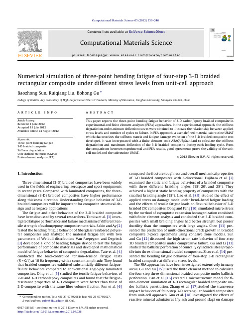
The FEA approaches have been investigated extensively in many areas. Gu and Xu [15] used the ﬁnite element method to calculate the four-step three-dimensional braided composite under ballistic perforation. Lian et al. [16] created a microstructure model for ﬁnite-element simulation of 3-D rectangular braided composite under ballistic penetration. Zhang et al. [17]studied the transverse impact behaviors of four-step 3-D rectangular braided composites from unit-cell approach. Guo et al. [18] investigated the effects of reactive mineral admixtures (ﬂy ash and ground slag) on damage
compared the fracture toughness and overall mechanical properties of 3-D braided composites with Z-directional. Fujihara et al. [7] examined the static and fatigue behaviors of a braided composite with three different braiding angles (15°, 20°, and 25°). They achieved a highest static bending property of composites with the smallest braiding angle (15°). Liao et al. [8,9] studied the effect of applied stress on damage mode under bend–bend fatigue loading and the effects of tensile fatigue loads on ﬂexural behavior of 3-D braided C/C composites. Dong and Feng [10] simulated micro stress by the method of asymptotic expansion homogenization combined with ﬁnite element analysis and concluded that 3-D braided composites with small braiding angles had better strength but poorer ductility than the composites with large angles. Chen [11] presented the prediction of multi-directional crack growth in braided composite T-piece specimens using cohesive zone models. Sun and Gu [12] discussed the high strain rate behavior of four-step 3D braided composites under compressive failure. Gu and Li [13] studied the ballistic perforation of conically cylindrical steel projectile into three-dimensional braided composites. Zhao et al. [14] presented the bending fatigue behavior of four-step 3-D rectangular braided composite at different stress levels.

Full scale

AbstractAnalysis of full-scale measurements obtained from the instrumented Smedvig West Epsilon jack-up platform operating in the STATOIL Sleipner Vest "eld in the North Sea is described. This jack-up platform has a skirted spud-can foundation. The following topics are discussed in the paper:i Comparison between measured and calculated natural frequencies and modes of the plat- form based on modal analysis.i Comparison of measured foundation sti!ness with the design sti!ness.i Comparison between measured and simulated platform response by application of a nonlin- ear time domain analysis. Implications with respect to procedures and assumptions em-ployed for design of the platform are addressed.The comparison between measured and simulated response is performed for a moderate sea state with a signi"cant wave height of 9.3 m. 1999 Elsevier Science Ltd. All rights reserved.描述了从在北海的STATOIL Sleipner Vest字段中操作的仪表化的Smedvig西Epsilon自升式平台获得的全尺寸测量的分析，该自升式平台具有裙状定位桩基座。

专业英语

数学建模就是用数学语言描述实际现象的过程。是一种数学的思考方法，是运用数学的语言和方法，题的一种强有力的数学手段。
Mathematical model is a simulation, with mathematical symbols, mathematical formulas, programs, graphics, etc. on the actual topics essential attribute of abstract but simple characterizations, which may explain some objective phenomenon, or can predict the future development of the law , or to provide some kind of optimal strategy or a better strategy for the control of development in the sense of a phenomenon
数学模型是一种模拟，是用数学符号、数学式子、程序、图形等对实际课题本质属性的抽象而又简洁的刻划，它或能解释某些客观现象，或能预测未来的发展规律，或能为控制某一现象的发展提供某种意义下的最优策略或较好策略。
Mathematical models are generally not a direct replica of the real problem, which often requires both building awareness of the reality of the issue in-depth subtle observation and analysis, they need people to flexibly clever use of a variety of mathematical knowledge. This application of knowledge from the actual issues in the abstract, mathematical model of the process to extract called mathematical modeling.

SPH numerical and experimental modeling

Wave interaction with a vertical wall:SPH numericaland experimental modelingE.Didier n,D.R.C.B.Neves,R.Martins,M.G.NevesNational Laboratory for Civil Engineering,Av.do Brasil101,1700-066Lisbon,Portugala r t i c l e i n f oArticle history:Received31January2013Accepted22June2014Keywords:Smoothed particle hydrodynamics(SPH)Wave-structure interactionCoastal engineeringImpact loadsPhysical modelinga b s t r a c tPrediction of wave forces on caisson-type breakwaters is challenging,especially in the case of impactloads that strongly depend on wave reﬂection,and wave breaking which affects the wave characteristicsnear the structure.In recent years,numerical models have been further developed and their use isbecoming increasingly attractive,such as the Smoothed Particle Hydrodynamics(SPH)numerical modelswhich enable the simulation of complex free surfaceﬂows.The SPH numerical model developed at theNational Laboratory for Civil Engineering(LNEC)is validated by comparing the numerical results of thewave interaction with a vertical wall using data obtained from physical modeling tests carried out in oneof the LNEC'sﬂumes.The numerical results presented a good agreement with the physical model tests.The free surface level was well estimated,with a concordance index between numerical results andexperimental data of about90.5–99.1%,presenting an average value of95.5%.Pressure at the verticalwall shows high intensity and short duration impact loads,and presented a concordance index betweennumerical results and experimental data about68.8–94.4%,with an average value about86.2%.Considering the complex phenomena involved,which is highly difﬁcult to be accurately modeled,numerically and experimentally,a good agreement between physical tests and numerical results wasaccomplished.&2014Elsevier Ltd.All rights reserved.1.IntroductionThe prediction of wave forces on caisson-type breakwaters isvery difﬁcult,especially in the case of impact loads that stronglydepend on wave reﬂection and wave breaking,which affect thewave characteristics near the structure(PROVERBS,1999).The impactloads present high intensities for short periods,often closer to1/100times a period,and are strongly inﬂuenced by the air effects while“pulsating”or while the“quasi-static”loads occur with durationsaround0.2–0.5times a wave period(Cuomo et al.,2010).The forces on a vertical wall of a breakwater are usuallypredicted by using a semi-empirical formula or by physicalmodeling.However,numerical modeling is becoming an attractivetool for calculating forces on coastal structures.Nevertheless,onlyfew numerical models allow simulating the complex phenomenaof wave breaking and overtopping,and consequently forces atvertical structures.Some examples of model applications tosimulate the pressure at vertical structures are the2D RANS modelCOBRAS-UC(Lara et al.,2008,Guanche et al.,2009)or,morerecently,a3D RANS model application of OPENFOAM@(Higueraet al.,2014)based on Volume of Fluid(VoF)approach,or a2DRANS Particle Finite Element Method(PFEM)(Oñate et al.,2004).Models,based on a Lagrangian method,such as the SmoothedParticle Hydrodynamics(SPH),have emerged recently and are avery interesting option for modeling complex free surfaceﬂows.The SPH method is based on the Lagrangian formulation of theNavier–Stokes equations and on a completely mesh-free technique.Based on this technique,different models and several numericalimplementations have been developed(Crespo,2008;Gotoh et al.,2001;Shao,2010).The weakly-compressible SPH(WCSPH)model used at theNational Laboratory for Civil Engineering(LNEC)is based on theoriginal SPHysics model(Gómez-Gesteira et al.,2008,2012;SPHysics code v1.4,2009)inspired by the formulation ofMonaghan(1992),and has been especially improved for model-ing waves interacting with coastal structures(Didier and Neves,2008,2009a,2009b,2010a,2010b,2012;Didier et al.,2011,2013;Neves et al.,2012).This paper presents the validation of the weakly-compressibleSPH numerical model for the study of the wave interaction with avertical wall.In order to accomplish this goal,a set of physicalmodel tests were performed at LNEC in a waveﬂume with theContents lists available at ScienceDirectjournal homepage:/locate/oceanengOcean Engineering/10.1016/j.oceaneng.2014.06.0290029-8018/&2014Elsevier Ltd.All rightsreserved.n Corresponding author.Tel.:þ351218443904;fax:þ351218443011.E-mail addresses:edidier@lnec.pt(D.E.),dneves@lnec.pt(N.D.R.C.B.),ricardomartins3@(M.R.),gneves@lnec.pt(N.M.G.).Ocean Engineering88(2014)330–341experimental set-up and boundary conditions identical to the numerical model:the ﬂume dimensions and the piston-type wave-maker movement are the same for both numerical and physical model.The accuracy of the numerical model was assessed,particularly regarding two phenomena:wave propaga-tion,and wave impacts on the vertical wall.2.SPH numerical modelThe Smoothed Particle Hydrodinamics (SPH)numerical meth-ods were initially applied to astrophysics by Gingold and Monaghan (1977)and Lucy (1977)and later to hydrodynamics by Monaghan (1992,1994).The SPH method is a completely mesh-free technique,enabling the modeling of the ﬂuid particles trajectories accordingly to the Navier –Stokes equations written on the SPH formalism,based on the theory of interpolation integrals which use interpolation kernels.The Lagrangian approach of the SPH methods consists in following the ﬂuid particles in a determined time interval in order to obtain its trajectories,velocities and pressures as a function of the initial position and time.2.1.Principle of the SPH methodThe fundamental principle of the SPH methods is to approx-imate a scalar,a function or a tensor using the theory of the interpolation integrals.The integral of an interpolation function f (r )is given by the following equation:f ðr Þ¼Zf ðr 0ÞW ðr Àr 0;h Þdr 0ð1Þwhere r is the vector particle position,W is the weighting function,called kernel,h is the smoothing length.The kernel allows determining the interaction among neighboring particles included in their in ﬂuence domain.This domain is a compact support within a circular region determined by a radius of 2h ,controlled by the smoothing length h ,de ﬁned as h ¼0.92n 20.5d 0,with d 0the initial particle spacing.The kernel is an analytic function which can be differentiated without requiring any spatial mesh.Numerically,the function f (r )is only known at the particles,and the interpolation integrals are approximated by the sum of the contribution of each particle included in their in ﬂuence domain.The function is written as an approximation of the function f at a particle a at the position r a ,and is given by the following equation:f ðr a Þ%∑bm bf bρbW ab ð2Þwhere f b is the value of the function f associated with the particle b at r b ,W ab ¼W (r a Àr b ,h )is the value of the kernel at (r a Àr b ),m b and ρb are the mass and the density of the particle b ,respectively.For numerical simulation of wave propagation,the quadratic kernel (Johnson et al.,1996;Dalrymple and Rogers,2006)is used to determine the interaction between the particles.This kernel is de ﬁned by the analytic function:W ðq ;h Þ¼32πh q2Àq þ1 ð3Þwhere q ¼(r a Àr b )/h and 0r q r 2.This kernel has the particularity of not having an in ﬂection point in its ﬁrst and second derivative in the range of the function de ﬁnition.2.2.Set of equations in Lagrangian formThe 2D momentum conservation equation and the conserva-tion law,in Lagrangian form,for a viscous ﬂuid are written asfollow:d v d t ¼À1ρ∇P þΠþg ð4Þ1ρd ρd t¼Àdiv ðv Þð5Þwhere t refers to the time,v the velocity,P the pressure,ρthe ﬂuid density,Πthe viscous terms and g ¼(0,À9.81)m/s 2the gravita-tional acceleration.The standard SPH formulation (Monaghan,1994),in which the ﬂuid is considered weakly-compressible,is used and the pressure is calculated by an equation of state (Batchelor,1974)through the ﬂuid densityP ¼B ρρ0 γÀ1with B ¼c 20ρ0γð6Þwith γ¼7,ρ0is the reference density and c 0the speed of sound at the reference density.The particle trajectories are obtained from the following relationship:d r d t¼v ð7Þwhere r is the particle position.Classically,the XSPH method (Monaghan,1989)allows the movement of the particles with a velocity similar to the average of their neighborhood.However,the XSPH method can introduce some undesirable numerical arti ﬁcial viscosity and numerical instabilities during the wave propagation,also some particles aquire enough velocity to cross the solid boundaries (Didier and Neves,2009b ).Thus the XSPH correction is not used in SPHyCE.2.3.SPH numerical modelThe SPH numerical model used at LNEC is based on the open-source code SPHysics (Gómez-Gesteira et al.2008,2012),version 1.4(Crespo,2008;SPHysics code v1.4,2009),inspired by the SPH standard formulation of Monaghan (1994).The ﬂuid in the standard SPH formalism is treated as weakly-compressible,allow-ing the direct pressure calculation through a state equation (Batchelor,1974),that relates the ﬂuid pressure with the density.The LNEC's SPH numerical model is speci ﬁcally improved for coastal engineering problems,complex free surface ﬂows and wave interacting with impermeable and porous coastal structures.In the SPH equations,the discrete equation of the momentum conservation is given by the following equation:D v a ¼∑b m b P a ρa þP bρb þΠab !∇a W ab þg ð8Þwhere v a ,P a and ρa are the velocity,pressure and density of a particle a ,respectively,P b ,ρb and m b are the pressure,density and mass of a particle b ,respectively,included in the in ﬂuence region of the kernel,W ab is the kernel and Πab the viscosity term.Finally,∇a W ab is the kernel gradient.The turbulence model sub-particle scale (SPS)(Gotoh et al.2001)is used since it includes not only a viscosity model but also the turbulence effect through a model derived from the LES-type models (Large Eddy Simulation).The arti ﬁcial viscosity model (Monaghan,1992),with two empirical parameters that should be calibrated,is frequently used to stabilize the numerical process but introduces a numerical diffusion that might affect signi ﬁcantly the wave amplitude (Didier and Neves,2009b ).D.E.et al./Ocean Engineering 88(2014)330–341331The mass conservation equation in the discrete SPH formalism is given by the following equation:D ρaD t ¼∑bm b ðu a Àu b Þ∇a W ab ð9ÞThe particles move according to the following equation:D r a¼u a ð10ÞThe pressure is obtained by the equation of state,given by Eq.(6).For numerical reasons,the sound velocity c 0must be high enough to reduce ﬂuctuations due to density and low enough to allow the model to run with a reasonable calculation time step.Therefore,it is usually considered,for the calculations,a sound velocity signi ﬁcantly lower than its classic value (Monaghan,1994;Gomez-Gesteira et al.,2012).The ﬂow kinematics of the SPH models is generally realistic.However,a problem inherent to the weakly-compressible SPH (WCSPH)formulation,based on the formulation of Monaghan (1994),is that the particle pressure might exhibit large oscillations.Gómez-Gesteira et al.(2010)shows that ﬁltering density (i.e.renormalization of particle density)allows to obtain a pressure ﬁeld without oscillations and a good representation of a dam-break ﬂow.However,ﬁltering density in ﬂuence seems to be more complex for wave propagation.Hughes and Graham (2010)com-pared incompressible SPH (ISPH)and WCSPH models,with and without ﬁltering density,for waves impacting on a vertical wall.Both methods have shown to be able of simulating the pressure on the vertical wall due to the wave impacts.The predictions for the wave impacts have shown to be in agreement,qualitatively and quantitatively,with the available experimental data.Results from the WCSPH appear to be signi ﬁcantly smoother than those from ISPH.This is particularly the case for the free surface deformation and especially for the wave breaking.Preliminary studies (Didier et al.,2011,2013;Martins,2012)comparing numerical and experimental results for wave impact on a vertical breakwater showed that the conventionally used density ﬁlter stabilizes the pressure ﬁeld but causes a numerical diffusion on wave propaga-tion and a consequent reduction on wave height that is not observed in the experimental results.On the other hand,without the density ﬁlter,pressure oscillations appear and forces on structures are more dif ﬁcult to be calculated.With these results,a partial ﬁltering density technique,i.e.renormalization applied only for particles near the structure,was developed allowing to simultaneously propagate waves without diffusion and to model accurately the pressure ﬁeld near the structure.The pressure instabilities can be resolved by correcting the kernel function,recalculating the value of the particle density.The application of the density renormalization is performed every 30iterations of time (classical value)applying the Shepard ﬁlter (Colagrossi and Landrini,2003).The new density value of a given particle is calculated by the following equation:ρa ¼∑bm b ~W abð12Þ~Wab ¼W abbW ab m bρbð13ÞIn the LNEC's SPH model,the time integration is performed usingthe predictor-corrector algorithm (Monaghan,1989).The time step is automatically controlled accordingly to the CFL conditions proposed by Monaghan and Kos (1999).The particle velocity is calculated using the discrete equation of the momentum conser-vation,Eq.(8),the density is set by the discrete form of the continuity equation,Eq.(9),and the position of the particles iscalculated by Eq.(10).The pressure is calculated from the density using the Tait equation,Eq.(6).Detail of numerical implementation is available in Gómez-Gesteira et al.(2008,2012),SPHysics code v1.4(2009)and Didier and Neves (2009b,2012),Didier et al.(2013).2.4.Boundary and initial conditionsThe boundary conditions are not displayed directly in the SPH formalism.In the present model the repulsive boundary condition,developed by Monaghan and Kos (1999)and corrected by Rogers and Dalrymple (2008),that imposes a repulsive force from the solid particles of the boundary to the ﬂuid particles,is used and allows preventing the water particles to cross the solid boundary.Initially,the water particles are placed in the ﬂume using a regular Cartesian distribution,i.e.particles are regularly distrib-uted,with the spacing between particles de ﬁned by d o .This is a condition of the SPH method when the smoothing length of the kernel is constant.The distribution of the solid particles at boundaries follows the one adopted for the ﬂuid particles,namely the distance between the particles is equal to d o independently of the direction of the boundaries.The velocity ﬁeld is zero and the pressure is hydrostatic.The particle density is equal to the water density,1000kg/m 3.Regular incident waves were generated using a piston-type wave-maker,with the same motion as in the experimental tests,by moving the solid particles of left boundary of the SPH numerical domain (Crespo et al.,2008).3.Physical modeling of wave impact on a vertical wall Within the aim of validating the SPH numerical model,physical tests of waves interacting with a vertical breakwater were per-formed in one of the LNEC's ﬂume with 49.4m length,1.6m wide and 1.2m height.The ﬂume is equipped with a piston-type wave-maker and is able to generate both regular and irregular waves.The physical model set-up was determined in such a way that was feasible the exact replication in the numerical model,taking into account the characteristics of the numerical model,and to ensure that conditions for numerical and experimental models were identical.The coastal structure consists on an impermeable vertical breakwater composed by a 0.181m height berm with a 1:3slope,and a 0.03m thickness acrylic vertical wall.The vertical wall was reinforced by vertical supports on its rear part to ensure rigidity of the structure,and was located 0.2m from the top of the slope,asitFig.1.Schematic representation of the wave ﬂume and the structure and itsdimensions.D.E.et al./Ocean Engineering 88(2014)330–341332is shown in Fig.1.The crest freeboard is 0.385m above the berm.The horizontal bottom between the piston-type wave-maker and the beginning of the 1:3slope was 3.62m length.The case analyzed in the present paper is an incident regular wave with a wave period,T ¼1.3s,and a wave height,H ¼0.10m.Interaction between regular wave and vertical breakwater was analyzed for four different water depths,d ,varying from 0.325m to 0.266m,which result in wave lengths,L ,from 2.023m to 1.879m (Martins,2012).For these conditions,it is expected to have an impact load for all cases,according to PROVERBS (1999).Table 1presents the characteristics of the four analyzed con ﬁg-urations:the wave length,the wave-maker amplitude,A b ,and the water depth at the toe of the vertical breakwater,d t .The tests lasted long enough to generate at least ten regular waves.Active absorption of the re ﬂected waves at the wave-maker was not considered in the present tests since it was not implemented at the numerical model at the stage.Experimental data was collected in two resistive-type wave gauges (developed at LNEC),and six pressure sensors (model AB/HP from Honeywell with diaphragm size of 19mm and maximum pressure 20,000PSI).The ﬁrst gauge (G1)was located at x ¼2.643m from the wave-maker initial position to verify the generated wave characteristics.The second gauge (G2)was located on the 1:3slope,at x ¼3.943m,to verify wave conditions near the structure.Six pressure sensors were located at the front face of the vertical wall,approximately at the middle of the wall width,to limit the effects of the ﬂume walls.The center of pressure sensor P1is located 0.055m above the berm.The center of sensor P2is placed 0.055m above the center of P1,the center of P30.055m above the center of P2,etc.(Fig.1).Fig.2shows the wave ﬂume with the vertical wall and the sensor position.Eventhough a sampling rate greater than 1kHz is recom-mended to measure impact pressure,a frequency of 400Hz was used for data acquisition in both wave gauges and pressure sensors due to the available equipment limitations.Each wave condition was repeated ten times.The several repetitions present a good agreement:before wave re-re ﬂection on the wave-maker for the four con ﬁgurations and for free surface elevation,the maximum deviation,RMS (root-mean-square),ofthe repetitions (Table 2)were 70.0017m and 70.0058m at gauges G1and G2,respectively.Errors were larger for G2,the gauge located near the structure,since there stronger non-linear phenomena appear.The second part of Table 2presents the relative errors,i.e.the percentage of variation expressed as the ration between the RMS and the wave amplitude.The calculated errors are less than 6%for gauge G1and between 6%and 11%for gauge G2due to the proximity of the structure.Table 3presents the maximum deviation of the pressure values for the repetitions at P1to P6and for the four con ﬁgurations.Overall pressure deviation shows a good agreement despite its higher RMS values,ranging from 0.82Â10À2m H 2O to 9.59Â10À2m H 2O.Values of RMS were larger for the pressure sensor that was directly exposed to the impact loads (sensor P1for con ﬁgurations 1and 2and sensor P2for con ﬁguration 3and 4).The phenomena involved (impact loads)and the high turbulent nature of the ﬂow combined with the very short duration of the pressure peaks and the variability of the impact point are some reasons for these higher values.Tables 4,6,8and 10and 5,7,9and 11present the ﬁrst maximum pressure and corresponding RMS at sensors for the ﬁrst wave impact/interaction on the structure and the correspondingTable 1Characteristics of the four studied con ﬁgurations of the vertical breakwater.Con ﬁguration d (m)L (m)A b (m)d t (m)10.266 1.8790.057650.08520.282 1.9210.055180.10130.300 1.9650.052960.11940.3252.0230.050480.144posite breakwater at the ﬂume with pressure sensors at the front face.Table 2RMS of free surface elevation at gauge G1and G2and percentage of variation expressed as the ration between the RMS and the wave amplitude.RMS (m)Â10À3Con ﬁguration 1234G1 1.717 2.849 2.452 2.391G2 5.763 5.147 3.342 3.625Error %1234G1 3.43 5.70 4.90 4.78G211.5310.296.687.25Table 3RMS of pressure at sensors P1to P 6.RMS (mH 2O)Â10À1Con ﬁguration 1234P10.679 1.0490.7370.111P20.2930.7860.8940.121P30.1830.2230.1260.111P40.1350.1540.1280.087P50.1230.1320.0990.095P60.1340.1440.1230.088D.E.et al./Ocean Engineering 88(2014)330–341333percentage of variation expressed as the ratio between the RMSand the maximum pressure at the sensors,respectively.The errors obtained for theﬁrst pressure peak(maximum),corresponding to theﬁrst impact or interaction between the incident wave and the vertical wall,present values ranging from10%to50%.These values indicate the variability of the complex phenomenon which occurs during wave-structure interaction that can vary between test repetitions.This fact demonstrates the difﬁculty to reproduce numerically the measured pressure.Differences on the free surface level and on the pressure were larger after the re-reﬂection phenomena on the wave-maker and were not considered for the present analysis.4.Numerical modeling of wave impact on a vertical wallThe weakly-compressible SPH numerical model was used for modeling impact loads on a vertical wall.Wave generation was performed by a piston-type numerical wave-maker with the same amplitude of the sinusoidal movement imposed at the physical model.The partialﬁltering density technique was applied to particles from x¼4.086m(middle of the1:3slope)to the end of the numerical domain(Martins,2012;Didier et al.,2013)and each30 time iterations(Gómez-Gesteira et al.,2008).Table4Maximum pressure and RMS at sensors P1–P3for wave impact for case1 (d¼0.266m).Pressure sensor(mH2O)Â10À1Wave impact123P1P Max 3.93 1.71 1.91RMS0.6790.6360.584 P2P Max 1.170.820.84RMS0.2930.1610.152P3P Max 1.050.930.81RMS0.1830.1960.136Table5Percentage of variation expressed as the ration between the RMS and the maximum pressure at sensors P1–P3for the wave impact at case1(d¼0.266m).Pressure sensor Wave impact123P117.2837.1930.37 P225.0419.6318.10P317.4321.0817.00Table6Maximum pressure and RMS at sensors P1–P3for wave impact at case2 (d¼0.282m).Pressure sensor(mH2O)Â10À1Wave impact123P1P Max 1.39 3.33 4.12RMS0.2040.569 1.049 P2P Max 1.62 1.31 1.56RMS0.7860.4200.262 P3P Max0.830.840.77RMS0.1590.2230.122Table7Percentage of variation expressed as the ration between the RMS and the maximum pressure at sensors P1–P3for wave impact at case2(d¼0.282m).Pressure sensor Wave impact123P114.6817.0925.46 P248.5232.0616.79 P319.1626.5515.84Table8Maximum pressure and RMS at sensors P1–P4for wave impact for case3 (d¼0.300m).Pressure sensor(mH2O)Â10À1Wave impact123P1P Max0.71 2.29 1.92RMS0.1100.5830.737 P2P Max0.83 2.11 2.54RMS0.0860.8940.365 P3P Max0.930.740.77RMS0.1260.0850.095 P4P Max0.790.0640.052RMS0.1280.0950.069Table9Percentage of variation expressed as the ration between the RMS and the maximum pressure at sensors P1–P4for wave impact at case3(d¼0.300m).Pressure sensor Wave impact123P115.5225.3538.49 P210.4042.3414.43 P313.5411.5612.35 P416.3714.8413.38Table10Maximum pressure and RMS at sensors P1–P4for wave impact at case4 (d¼0.325m).Pressure sensor(mH2O)Â10À1Wave impact123P1P Max0.6470.7370.758RMS0.0870.1080.111P2P Max0.7210.8050.732RMS0.0750.1210.094 P3P Max0.7940.6890.761RMS0.0970.1010.111P4P Max0.6310.8520.720RMS0.0620.0870.057Table11Percentage of variation expressed as the ration between the RMS and the maximum pressure at sensors P1–P4for wave impact at case4(d¼0.325m).Pressure sensor Wave impact123P113.4514.6514.64 P210.4215.1312.84 P312.2214.6614.61 P49.8410.247.92D.E.et al./Ocean Engineering88(2014)330–341 334For the present simulations the number of ﬂuid and solid particles used depended on the water depth in the ﬂume and is indicated in Table 12.Convergence study for the particle dimen-sions,performed by Didier et al.(2013),indicates that a resolution of at least 36–40particles per wave height is necessary for an accurate modeling of the wave propagation and impact loads on vertical wall.This criterion was respected in the present study to de ﬁne the number of the particles for each tested con ﬁguration.For case 1,d ¼0.266m,the total number of particles was 154735.For this case,the mean time step was around 2.4Â10Àputational time was 83h for modeling 8.5s,using a serial version of the code and a Personal Computer Intel (R)Core(TM)i7CPU 930@2.80GHz.The numerical and the physical modeling was performed without dynamic absorption of the wave-maker,so the result analysis was conducted before re-re ﬂection of the wave on the wave-maker reached the breakwater,corresponding to four wave impacts on the breakwater.Thus,the numerical simulations were performed until 8.5s.Figs.3–10show the mean time series of free surface elevation at gauges G1and G2,and pressure at sensors P1–P4,for the wave height H ¼0.10m,the wave period T ¼1.3s and for the water depth at the toe of the vertical breakwater,d t ,varying from 0.085m to 0.144m (Table 1).At sensors P5and P6less wave impact occurred,producing less relevant results for the analyses.Time series of the numerical results were compared with the average of the experi-mental data time series (i.e.average of the 10test repetitions).Figs.3,5,7,and 9present the time series of the numerical and experimental free surface elevations at gauges G1and G2.A good agreement was globally observed between numerical results andTable 12Dimension of particles,d o ,smoothing length,h ,and number of particles for the four con ﬁgurations.Con ﬁguration d (m)d o (m)h (m)No.of particles 10.2660.00266000.003460915473520.2820.00266040.003461416453030.3000.00265490.003454217632740.3250.00266390.0034660190465Fig.3.Free surface elevation for d ¼0.266m,(a)gauges G1(b)andG2.Fig.4.Pressure on sensor for d ¼0.266m,(a)P1,(b)P2,and (c)P3.Fig.5.Free surface elevation for d ¼0.282m,(a)gauges G1and (b)G2.D.E.et al./Ocean Engineering 88(2014)330–341335experimental data for gauges G1and G2:for all the tested water depths the free surface elevation pattern was correctly simulated.The differences between numerical and experimental results atgauges G1and G2were slightly larger for the crests and troughs.For the percentage of variation,expressed as the ratio between the RMS and the wave amplitude,the same trend was observed comparing numerical and experimental results (Table 2and 13).Figs.4,6,8and 10present the time series of numerical and experimental pressure at the pressure sensors P1,P2and P3(Figs.4and 6)and P1,P2,P3and P4(Figs.8and 10).Numerical pressure time series exhibit some noise,even when using the partial re-normalization of particle density and a ten pass of smoothing was applied using an average smoothing on ten neighboring points.Pressure variation trend at sensors P1–P4obtained with the numer-ical model was globally similar to the experimental data.Agreement between numerical and experimental results was goodregardingFig.6.Pressure on sensor for d ¼0.282m,(a)P1,(b)P2,and (c)P3.Fig.7.Free surface elevation for d ¼0.300m,(a)gauges G1and (b)G2.Fig.8.Pressure on sensor for d ¼0.300m,(a)P1,(b)P2,(c)P3,and (d)P4.D.E.et al./Ocean Engineering 88(2014)330–341336。

Numerical simulation of pulverized coal MILD combustion considering advanced heterogeneous

Turbulence,Heat and Mass Transfer7c 2012Begell House,Inc.Numerical simulation of pulverized coal MILD combustion considering advanced heterogeneous combustion modelM.Vascellari1,2,S.Schulze1,D.Safronov1,P.Nikrytyuk1,C.Hasse11ZIK Virtuhcon,Dep.of Energy Process Enginnering and Chemical Engineering,University of Technology Freiberg,Fuchsmhlenweg9,09599Freiberg,Germany2Michele.Vascellari@vtc.tu-freiberg.deAbstract—A new advanced subgrid scale(SGS)model for coal particle combustion and gasiﬁcation was devel-oped.The new model considers a detailed representation of the diffusion and convection phenomena in the direct proximity of the coal particle,which are generally neglected by standard models available in literature.This paper shows the coupling of the new model with the commercial CFD code Ansys-Fluent and its validation consider-ing a full-scale furnace.In particular the IFRF pulverized coal MILD combustion experiments are considered for validating the results of the new model,showing a better agreement with experiments with respect to a standard model.1.IntroductionNew“clean coal technologies”for reducing pollutants from coal power plants require new advanced design tools,able to accurately predict the performances and the emission of such systems.CFD simulations represent a very important tool for designing advanced coal conversion system.However,coal combustion and gasiﬁcation require several mathematical submodels to represent the several chemical physical phenomena involved.Subgrid scale models are gener-ally developed and validated considering small scale experimental test,focusing the attention on only one ually,it is diffult to extrapolate the results of small scale laboratory tests to large scale system because of the complex nature of turbulent,reacting and multiphase ﬂows in such systems.Eaton et al.[1]presented an overview of the main submodels required for modelling solid fuels systems and their application to comprehensive CFD models.This work presents the coupling of a new subgrid scale(SGS)model for coal char com-bustion with a CFD code and its validation considering a semi-industrial scale pulverized coal MILD test-case[2].The new models was previously developed and validated considering sin-gle coal particle direct numerical simulations(DNS)[3].The new model showed excellent agreement with single particle DNS,predicting enhanced char conversion rates with respect to standard Baum and Street[4]model.2.Numerical ModelsDuring coal combustion several chemical-physical phenomena take place.They require spe-ciﬁc mathematical models implemented in a comprehensive CFD code[1].The main models considered concern the following phenomena:turbulence,multiphaseﬂow and interphase in-teractions,homogeneous and heterogeneous chemical reactions,radiation,etc..Simulations of MILD coal combustion were performed considering the commercial CFD code Ansys-Fluent,version13.0.The Reynolds Average Navier Stokes(RANS)equations are2Turbulence,Heat and Mass Transfer7Table1:Experimental conditions of IFRF furnace[2]Massﬂowrate,kg/hTemp.,K Composition(%vol)PrimaryAir130313.15O221%,N279%Secondary air 6751623.15CO28.1%,O219.7%,N257.2%,H2O15.1%solved on an unstructured hybrid mesh using aﬁnite volume discretization approach.The three-dimensional version of the pressure-based solver is considered.The SIMPLE[5]algorithm is used for velocity-pressure coupling.Convectiveﬂuxes in all transport equations are discretized with a second-order accurate upwind scheme and the pressure gradient with a second-order accurate scheme.The realizable k− turbulence model[6]is considered for RANS equations closure.The P-1radiation model[7]is considered for radiation heat transfer.The coal discrete phase is modelled considering a Eulerian-Lagrangian approach.The main gas phase is solved considering transport equations for continuous phase in the Eulerian frame of reference,while the secondary discrete solid coal phase is solved considering a Lagrangian frame.The trajectories of the particles are evaluated by integrating the force balance on them with respect to time.The continuous phaseﬂow pattern is impacted by the discrete phase(and vice versa)and the calculation of the main phase is alternated with the discrete phase until a converged coupled solution is achieved.As the trajectory of a particle is computed,the heat, mass and momentum gained or lost by the particle are evaluated,and these interactions are taken into account in the Eulerian equations of the primary phase by means of source terms. The dispersion of particles due to turbulence is taken into account by considering the stochastic tracking model,including the effect of instantaneous turbulent velocityﬂuctuations on particle trajectories.The interaction between turbulentﬂow and chemical reaction plays a fundamental rule in MILD combustion modeling,whether considering solid or liquid and gaseous fuels.Indeed,ﬂuid dynamic behaviour of MILD combustion strongly differs from conventional combustion, because gradients of temperature and chemical species concentrations are generally lower[8]. In this way,a well-deﬁnedﬂame front can no longer be observed.In particular,it was demon-strated[9]that better prediction of temperature and chemical speciesﬁeld were obtained consid-ering advanced turbulence-chemistry interaction model,such as EDC[10]with detailed kinetic mechanisms.The DRM mechanism[11]with103reactions among22chemical species is chosen here.Coal combustion is modelled according to the following sequence of phenomena:drying, pyrolysis,volatile combustion and char burnout.Moisture drying is governed by the difference of water concentrations between the parti-cle surface and the bulk phase.The water concentration on the particle surface is evaluated by assuming that the partial pressure of vapor at the interface is equal to the saturated vapor pressure at the particle temperature.The mass transfer coefﬁcient used for evaluating moisture evaporation is calculated by means of correlation of Ranz and Marshall[12].Pyrolysis can be regarded as a two-stage process[13].During primary pyrolysis,coal par-ticles decompose and release volatile matter(devolatilization),composed by TAR,light hy-drocarbons and gas.During secondary pyrolysis,TAR decomposes and produces soot,lightM.Vascellari et al.3Table2:Proximate and ultimate analysis of Guasare coal[2]Proximate analysis Ultimate analysis(%daf)V olatile matter37.1C78.41Fixed carbon56.7H 5.22Moisture 2.9O10.90Ash 3.3N 1.49LHV31.74MJ/kgTable3:V olatile yield predicted by CPD modelVolatile yield,%dafChar61.69TAR26.91H2O 5.51CO2 1.31CH4 2.26CO0.77N2 1.55hydrocarbons and gas.The devolatilization rate is modelled based on an empirical single ki-netic rate law[14].dY=A v exp(−E v/RT p)·(Y0−Y)(1)dtwhere T p is the particle temperature and Y and Y0are the instantaneous and the overall volatile yield on a dry ash-free(daf)basis,respectively.The model parameters A v and E v are the pre-exponential factor and the activation energy,which need to be adjusted for the given coal and the operating conditions.The CPD model[15]is used to determine the rate constants for single rate model.It requires chemical structure data from13C Nuclear Magnetic Resonance (13C NMR)spectroscopy on the speciﬁc coal.Since these detailed analysis data are usually not available,Genetti et al.[16]developed a non-linear correlation based on existing13C NMR data for30coals to determine the required(coal-structure-dependent)input data for the CPD model using the available proximate and ultimate analysis.This correlation is applied here. The volatile matter composition and the overall yield at high temperature were also estimated by means of the CPD model.V olatile matter is composed by light gases and hydrocarbons (CO,CO2,H2O,CH4,etc.)and heavy hydrocarbons(tar).Tar is approximated as an equivalent molecule C n H m,reacting with O2in the gas phase and producing CO and H2[13].2.1.Char Combustion ModelOnce volatile matter is completely released during primary pyrolysis,the char remaining in the coal particles reacts with the surrounding gas phase.The following four heterogeneous reactions were considered:4Turbulence,Heat and Mass Transfer7Figure1:Geometry of the IFRF furnaceC(s)+O2−→CO2(2)2C(s)+O2−→2CO(3)C(s)+CO2−→2CO(4)C(s)+H2O−→CO+H2O(5)Boudouard(Eq.(4))and gasiﬁcation(Eq.(5))reactions play an important role in MILD combustion[9,17]and they can not be neglected as usually is done for conventional coal com-bustion with atmospheric air.Char burnout is governed by the diffusion of the oxidant species from the bulk phase to the particle surface and by the heterogeneous reactions on the particle surface.Reaction rates are calculated considering global kinetic rates from[18,19].The diffusion of each chemical species from the bulk phase(∞)to the particle surface(s)is given by:β(c∞,i−c s,i)+4j=1νj,iˆR j=0(6)WhereˆR j is the rate of the reaction j,νj,i is the stoichiometric coefﬁcient of species i in reaction j andβis the mass transport coefﬁcient,calculated from the Ranz and Marshall[12] correlation,assuming unitary Lewis number.Generally,standard models[4]neglect the in-ﬂuence of the convection assuming stagnantﬂow around the particle.The diffusion of each species(Eq.(6))is equal to its production due to the heterogeneous reactions.The mass bal-ance of Eq.(6)account for the interactions between different surface reactions.In fact,CO2, produced on the particle surface from the char oxidization reaction(Eq.(2)),can react directly according to the Boudouard reaction(Eq.(4))increasing the overall char consumption.Gener-ally,standard models,such as[4]model,neglect any interaction between the different surface reactions.Further information about the model can beﬁnd in the paper of Schulze et al.[3].User Deﬁned Function(UDF)capability of Ansys-Fluent were used for coupling the SGS model,coded in C language,with the CFD solver,replacing the standard models for char com-bustion.5(a)(b)Figure 2:Comparison of temperature considering Baum and Street [4](BS)and SGS models respectively:(a)axial section contour plot;(b)radial proﬁles at 0.15,0.44,0.735,and 1.32m from the burner and comparison with experimental results [2].(a)(b)Figure 3:Comparison of CO dry volume fraction considering Baum and Street [4](BS)and SGS models respectively:(a)axial section contour plot;(b)radial proﬁles at 0.15,0.44,0.735,and 1.32m from the burner and comparison with experimental results [2].3.Validation of the SGS Char Combustion ModelValidation of SGS model was performed considering the experimental pulverized coal MILD test-case at the International Flame Research Fundation (IFRF)[2].MILD or ﬂameless com-bustion is a new technology developed for reducing pollutant emissions [8].Reactants are in-troduced at temperature generally higher than ignition temperature and the mixture is strongly diluted in order to reduce the temperature increase during reactions.The IFRF furnace is char-acterized by a square section of 2m ×2m and by a length of 6.25m,as shown in Fig.1.Primary air enters from the two lateral inlets,transporting pulverized coal particles.Secondary air is preheated by means of combustion with natural gas up to levels of 1350◦C before entering the furnace from the central inlet.Vitiated air is enriched with pure O 2in order to maintain the same concentration as atmospheric air.The furnace is ﬁred with 66kg h −1,130kg h −1and 675kg h −1respectively of coal,primary and secondary air,corresponding to a stoichiometric ratio of 1.2,as reported in Tab.1.The wall of the furnace is considered at the constant temper-Transfer7Figure4:Char consumption rate(kg/s m2)for65µm particles at0.44,0.735,1.32and2.05m from the burner.Results of Baum and Street(BS)model are reported on the left(triangles)and results of SGS on the right(circles)for each sectionsature of about1000◦C.The furnace isﬁred with Guasare coal,which proximate and ultimate analyisis are reported in Tab.2.Coal isﬁnely pulverized to give a particle size distribution with80%less than90µm[2].Particle size distribution is covered considering six classes[20]. V olatile yields are calculated by means of the CPD model,as reported in Tab.3.The single rate devolatilization model(Eq.(1))is calibrated by means of the CPD model,obtaining a pre-exponential factor of26353.9s−1and an activation energy of45.424kJ/mol.Considering recirculation of exhaust gas,the furnace is characterized by high concentrations of CO2and H2O and consequently a large fraction of char is converted through the gasiﬁcation (Eq.(4))and Boudoard(Eq.(5))reactions[17],representing an optimal test-case for validating the new char combustion model.The performances of the SGS model are therefore compared to the standard Baum and Street (BS)model andﬁnally validated against the experiments[2].Reactions Eq.(3)-(5)are consid-ered for Baum and Street model considering the same kinetic rates[18,19]used for the SGS model.Figure2(a)shows the comparison between the Baum and Street[4]and SGS models consid-ering the temperatureﬁeld.As expected,temperature gradients are very small and no clear front ofﬂame can be observed.Similar temperature proﬁles were predicted considering both models. The comparison with experiments is reported in Fig.2(b),considering four radial traverses at 0.15,0.44,0.735and1.32m from the burner.The SGS model predicts a lower temperature level in the inner jet zone,because of the increased conversion of char due to the endothermic reactions.Indeed,in this region,O2is almost completely consumed(see[9])and therefore only the endothermic gasiﬁcation(Eq.(5))and Boudouard reactions(Eq.(4))take place,absorbing heat from the gas phase.Figure3(a)shows the comparison of dry CO molar fraction on the axial section between the Baum and Street[4]and SGS models.Lower levels of CO are predicted by SGS model withrespect to Baum and Street model.Indeed,considering SGS model,the char reacting with O2 produces either CO either CO2,reducing the overall production of CO from the discrete phase. Dry CO molar fraction from numerical simulations is compared to experiments[2]considering four radial traverses at0.15,0.44,0.735and1.32m from the burner,as shown in Fig.3(b).SGS models shows a better agreement with respect to experiments.Figure4shows the char consumption rate at four cross sections for Baum and Street and SGS models considering65µm particles.As already observed for single particle simulations [3],SGS model predicts an enhanced char consumption rate with respect to Baum and Street model,nevertheless the same kinetic rates are used.In fact,the SGS model takes in account the inﬂuence of the heat and mass transport from the bulk phase to the particle surface and the interaction between the heterogeneous reaction in the particle boundary layer,enhancing the overall char consumption rate.4.ConclusionsIn this paper a new SGS model for char combustion,previously developed and validated for a single particle combustion by Schulze et al.[3],has been coupled to the commercial CFD code Ansys-Fluent and validated considering a pulverized coal MILD combustion test-case. The results have been compared to the standard Baum and Street model,used as default char combustion model by Ansys-Fluent.The comparison shows an improved prediction of the chemical species concentrations for the new SGS model with respect to the standard model. References[1]Eaton,A.et al.“Components,formulations,solutions,evaluation,and application ofcomprehensive combustion models”.In:Prog Energ Combust25.4(1999),pp.387–436.[2]Orsino,S.et al.Excess Enthalpy Combustion of Coal(Results of High Temperature AirCombustion Trials).Tech.rep.IFRF Doc.No.F46/y/3.International Flame Research Foundation,2000.[3]Schulze,S.et al.“Sub-model for a spherical char particle moving in a hot air/steamatmosphere”.In:Flow Turbul Combust(2012).(submitted).[4]Baum,M.et al.“Predicting the Combustion Behaviour of Coal Particles”.In:CombustSci Technol3.5(1971),pp.231–243.[5]Patankar,S.et al.“A calculation procedure for heat,mass and momentum transfer inthree-dimensional parabolicﬂows”.In:International Journal of Heat and Mass Transfer15.10(1972),pp.1787–1806.[6]Shih,T.et al.“A new k-epsilon eddy viscosity model for high reynolds number turbulentﬂows”.In:Computers and Fluids24.3(1995),pp.227–238.[7]Cheng,P.“Two-dimensional radiating gasﬂow by a moment method”.In:AIAA Journal2.9(1964),pp.1662–1664.[8]Cavaliere,A.et al.“Mild Combustion”.In:Prog Energ Combust30.4(2004),pp.329–366.[9]Vascellari,M.et al.“Inﬂuence of turbulence and chemical interaction on CFD pulverizedcoal MILD combustion modeling”.In:Fuel(2012).doi:10.1016/j.fuel.2011.07.042.[10]Gran I.,R.et al.“A numerical study of a bluff-body stabilized diffusionﬂame.Part1.Inﬂuence of turbulence modeling and boundary conditions”.In:Combust Sci Technol 119.1-6(1996),pp.171–190.[11]Kazakov,A.et al.Reduced Reaction Sets based on GRI-Mech1.2.http://me.berk/drm/.1994.[12]Ranz,M.et al.“Evaporation from drops:Part I”.In:Chem Eng Prog48(1952),pp.141–146.[13]F¨o rtsch,D.et al.“A kinetic model for the prediction of NO emissions from staged com-bustion of pulverized coal”.In:Proceedings of the27th Symposium(Intl.)on Combus-tion,The Combustion Institute,Pittsburgh27.2(1998),pp.3037–3044.[14]Badzioch,S.et al.“Kinetics of Thermal Decomposition of Pulverized Coal Particles”.In:Ind.Eng.Chem.Proc.Des.Dev.9.4(1970),pp.521–530.[15]Grant D.,M.et al.“Chemical model of coal devolatilization using percolation latticestatistics”.In:Energy&Fuels3.2(1989),pp.175–186.[16]Genetti,D.et al.“Development and Application of a Correlation of13C NMR Chem-ical Structural Analyses of Coal Based on Elemental Composition and V olatile Matter Content”.In:Energy&Fuels13.1(1999),pp.60–68.[17]Stadler,H.et al.“On the inﬂuence of the char gasiﬁcation reactions on NO formation inﬂameless coal combustion”.In:Combustion and Flame156.9(2009),pp.1755–1763.[18]Libby P.,A.et al.“Burning carbon particles in the presence of water vapor”.In:Com-bustion and Flame41.0(1981),pp.123–147.[19]Caram H.,S.et al.“Diffusion and Reaction in a Stagnant Boundary Layer about a CarbonParticle”.In:Industrial&Engineering Chemistry Fundamentals16.2(1977),pp.171–181.[20]Kim,J.et al.“Numerical modelling of MILD combustion for coal”.In:Progress in Com-putational Fluid Dynamics(2007).。

1、下载文档前请自行甄别文档内容的完整性，平台不提供额外的编辑、内容补充、找答案等附加服务。
2、"仅部分预览"的文档,不可在线预览部分如存在完整性等问题,可反馈申请退款(可完整预览的文档不适用该条件!)。
3、如文档侵犯您的权益，请联系客服反馈,我们会尽快为您处理(人工客服工作时间：9:00-18:30)。

Abstract
The spiral plate heat exchanger (SHE) is widely used in plenty of industrial services in full counter current flow liquid-liquid heat exchange. We have produced a thermal modelling of the heat exchanges in both steady-state and time dependent eases with 2D spiral geometry, allowing computation with different materials, forced convective heat transfer models in turbulent flow and geometrical parameters options. We will display here some results in steady-state conditions in order to improve the exchanger performances. Keywords: finite difference, finite element, plane spiral, thermal exchanger, transient state
Equations and thermo-physical parameters
The heat flow is modelled in the direction normal to the metallic walls by conduction and forced convection so that the studs have no influence because they induce some turbulences in the direction normal to the heat flow. The spiral curvature causes turbulences known as Taylor-Gortler phenomenon, which increase the convective heat-transfer coefficient along the metallic wall. With the following hypothesis: incompressible fluids, no internal sources, no dissipation function, neglected longitudinal diffusion, uniform temperature across a channel, fully developed turbulent flow, isotropic metal, we can write heat conservation law [ 1]: pC ~ - + div(pCTV) = - div((I)ar + (t)qh) where the conductive heat flow inside metal:
* To whom aU correspondence should be addressed.
0368--4466/95/$ 4.00 9 1995 Akad~miai lO'add, Budapest
John Wiley & Sons, Limited Chichester
306
DEVOIS et al.: SPIRAL PLATE HEAT EXCHANGER
J. Thermal Anal., 44, 1995
Two different numeric approaches have been realised to model the heat exchanges: finite differences [2] (both steady-state and time dependent cases) and finite elements [5] (only steady-state). We will describe in this paper only the finite difference method being used in steady-state operation. The main problem in modelling is the particular geometry which imposes a netting by regular sectors (Fig. 5), the minimal amount of sectors by turn is imposed by the computing accuracy; the number of nodes increases quickly as the number of turns
h=~. N u
The Nusselt number which characterizes the forced convective heat transfer is modelled three ways: - The standard approach with the Colburn Petrukhov formula:
OT -->
_-:-> k
J. Thermal Anal., 44, 1995
308
D E V O I S et al.: S P I R A L P L A T E H E A T E X C H A N G E R
qc - - k grad (7) and the forced convective heat flow at the metal-fluid sublayer boundary:
Description of the spiral-plate heat exchanger
The heat exchanger (Fig. 1) is fabricated from two long strips of metal plate which are spaced apart and wound around an open, spilt center to form a pair of concentric spiral passages. Spacing is maintained uniformly along the length of the spiral by spacer studs welded to the plates. The hot fluid enters at the exchangers's center and flows towards the periphery in channel A, the cold fluid enters sideways to lower thermal losses and flows towards the center in channel B (Fig. 2). Channels are folded and welded at their terminations alternatively to give easy access for cleaning, therefore the cross section is not rectangular (Fig. 3).
-~@ = - h(Tfluid -
Twit)
The computation of the convective heat transfer coefficient is generally complex because it must take into account additional turbulences caused by the spiral curvature. We have:
Nu=O.O23.ge~176
with n = - 0.25 for cooling (la~>~) and n = - 0 . 1 1 for heating (~,<~tf). - The local approach which uses the local curvature radius rc of the channel
Pr D V Re Nu h T
fluid thermal viscosity (middle of the channel)/N.s.m -2 Prandtl number mass flow rate/kg.s -1 average speed/m.s -1 Reynolds number average Nusselt number in turbulent flow convective heat transfer coefficient/W.m-LK-1 temperature/~ TAo input hot temperature (inside)/~ TB~ input cold temperature (outside)/~ T~x mixture temperature of fluids/~ AT temperature variation input output in the channel/~
Fig. 1 Spiral heat exchanger SHE1
J. Thermal Anal., 44, 1995
DEVOIS et al.: SPIRAL PLATE HEAT EXCHANGER
307ane
:~B
B
_L__f_
2'a
Fig. 3 Axial plane
(Ito) [3]:
Nu = 0.021.Re~
~ (2-~r
" d t t " o.1